 Economic growth is closely linked to investment. In the short term, there is a demand-side effect: higher investment, by increasing aggregate demand, creates a multiplier effect. GDP rises and unemployment falls. Over the longer term, higher net investment causes a supply-side effect: industrial capacity and potential output rise. This will be from both the greater quantity of capital and, if new investment incorporates superior technology, from a greater productivity of capital.
One of the biggest determinants of investment is certainty about the future: certainty allows businesses to plan investment. Uncertainty, by contrast, is likely to dampen investment. Investment is for future output and if the future is unknown, why undertake costly investment? After all, the cost of investment is generally recouped over several months or year, not immediately. Uncertainty thus increases the risks of investment.
 There is currently great uncertainty in the USA and its trading partners. The frequent changes in policy by President Trump are causing a fall in confidence and consequently a fall in investment. The past few weeks have seen large cuts in US government expenditure as his administration seeks to dismantle the current structure of government. The businesses supplying federal agencies thus face great uncertainty about future contracts. Laid-off workers will be forced to cut their spending, which will have knock-on effect on business, who will cut employment and investment as the multiplier and accelerator work through.
There are also worries that the economic chaos caused by President Trump’s frequent policy changes will cause inflation to rise. Higher inflation will prompt the Federal Reserve to raise interest rates. This, in turn, will increase the cost of borrowing for investment.
Tariff uncertainty
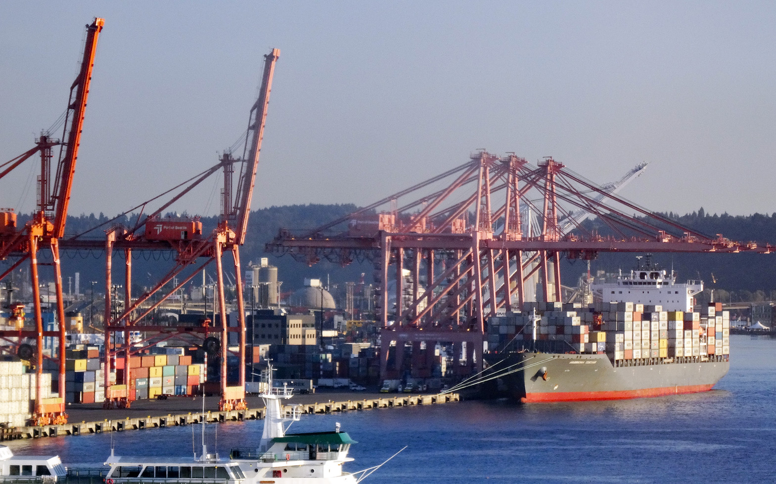 Perhaps the biggest uncertainty for business concerns the imposition of tariffs. Many US businesses rely on imports of raw materials, components, equipment, etc. Imposing tariffs on imports raises business costs. But this will vary from firm to firm, depending on the proportion of their inputs that are imported. And even when the inputs are from other US companies, those companies may rely on imports and thus be forced to raise prices to their customers. And if, in retaliation, other countries impose tariffs on US goods, this will affect US exporters and discourage them from investing.
For many multinational companies, whether based in the USA or elsewhere, supply chains involve many countries. New tariffs will force them to rethink which suppliers to use and where to locate production. The resulting uncertainty can cause them to delay or cancel investments.
Uncertainty has also been caused by the frequent changes in the planned level of tariffs. With the Trump administration using tariffs as a threat to get trading partners to change policy, the threatened tariff rates have varied depending on how trading partners have responded. There has also been uncertainty on just how the tariff policy will be implemented, making it more difficult for businesses to estimate the effect on them.
Then there are serious issues for the longer term. Other countries will be less willing to sign trade deals with the USA if they will not be honoured. Countries may increasingly look to diverting trade from the USA to other countries.
Video
Articles
- Trump’s erratic trade policies are baffling businesses, threatening investment and economic growth
Associated Press, Paul Wiseman, Anne D’innocenzio and Mae Anderson (6/3/25)
- The world is beginning to tire of Trump’s whiplash leadership
CNN, Stephen Collinson (6/3/25)
- US stocks slide and Nasdaq enters correction as chaos over Trump’s tariffs intensifies
CNN, John Towfighi (6/3/25)
- Trump’s Tariffs And Trade: Uncertainty, Chaos Or Brilliance?
Forbes, Mike Patton (6/3/25)
- How Trump’s second term might affect the market and your finances
The Conversation, Art Durnev (4/3/25)
- US corporate bond investors cautiously navigate trade war uncertainty
Reuters, Matt Tracy (6/3/25)
 This week in Trumponomics: Playing chicken with markets
Yahoo Finance, Rick Newman (8/3/25)
- Measuring fear: What the VIX reveals about market uncertainty
The FRED Blog, Aakash Kalyani (13/2/25)
- Trump shrugs off stock market slump, but economic warning signs loom
The Conversation, Conor O’Kane (17/3/25)
Data
Questions
- Find out what tariffs have been proposed, imposed and changed since Donald Trump came to office on 20 January 2025.
- In what scenario might US investment be stimulated by Donald Trump’s policies?
- What countries’ economies have gained or are set to gain from Donald Trump’s policies?
- What is the USMCA agreement? Do Donald Trump’s policies break this agreement?
- Find out and explain what has happened to the US stock market since January 2025. How do share prices affect business investment?
- Which sector’s shares have risen and which have fallen?
- Using the Data link above, find out what has been happening to the US Policy Uncertainty Index since Donald Trump was elected and explain particular spikes in the index. Is this mirrored in the global Policy Uncertainty Index?
- Are changes in the Policy Uncertainty Index mirrored in the World Uncertainty Index (WUI) and the CBOE Volatility Index: VIX?
 We continue to live through incredibly turbulent times. In the past decade or so we have experienced a global financial crisis, a global health emergency, seen the UK’s departure from the European Union, and witnessed increasing levels of geopolitical tension and conflict. Add to this the effects from the climate emergency and it easy to see why the issue of economic uncertainty is so important when thinking about a country’s economic prospects.
In this blog we consider how we can capture this uncertainty through a World Uncertainty Index and the ways by which economic uncertainty impacts on the macroeconomic environment.
World Uncertainty Index
Hites Ahir, Nicholas Bloom and Davide Furceri have constructed a measure of uncertainty known as the World Uncertainty Index (WUI). This tracks uncertainty around the world using the process of ‘text mining’ the country reports produced by the Economist Intelligence Unit. The words searched for are ‘uncertain’, ‘uncertainty’ and ‘uncertainties’ and a tally is recorded based on the number of times they occur per 1000 words of text. To produce the index this figure is then multiplied up by 100 000. A higher number therefore indicates a greater level of uncertainty. For more information on the construction of the index see the 2022 article by Ahir, Bloom and Furceri linked below.
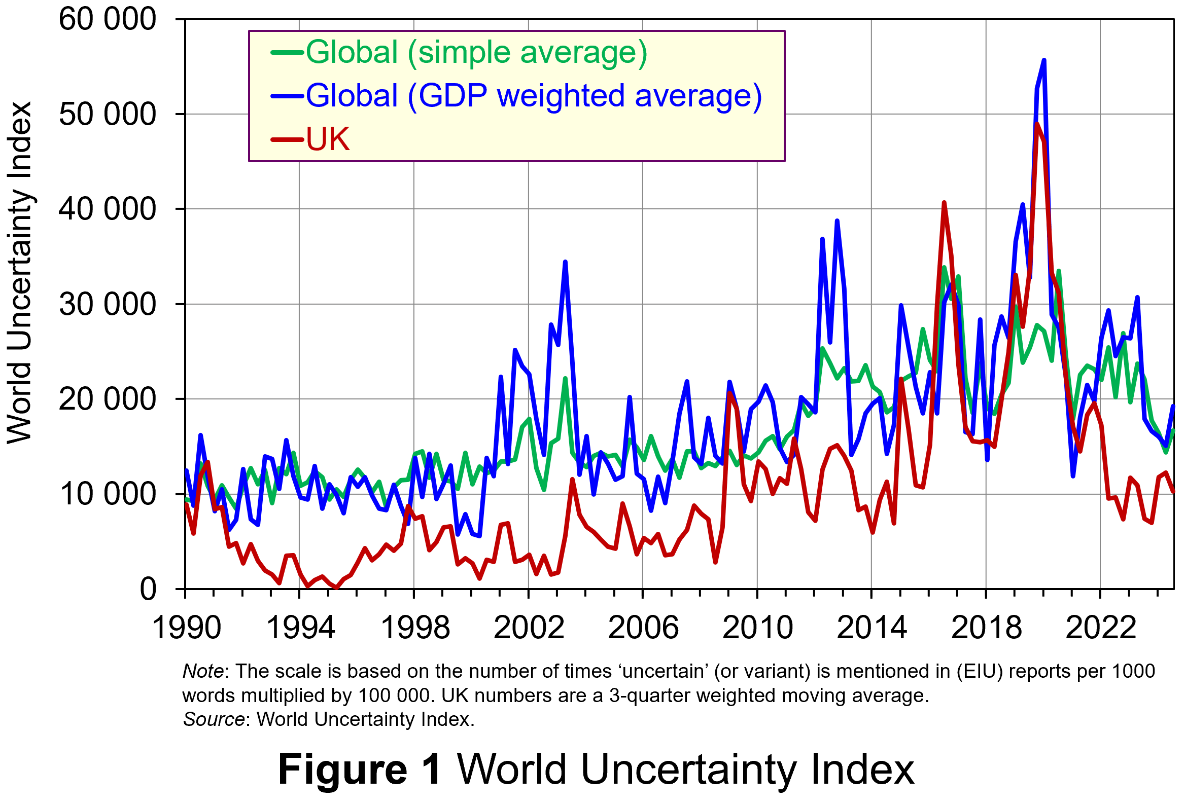 Figure 1 (click here for a PowerPoint) shows the WUI both globally and in the UK quarterly since 1991. The global index covers 143 countries and is presented as both a simple average and a GDP weighted average. The UK WUI is also shown. This is a three-quarter weighted average, the authors’ preferred measure for individual countries, where increasing weights of 0.1, 0.3 and 0.6 are used for the three most recent quarters.
From Figure 1 we can see how the level of uncertainty has been particularly volatile over the past decade or more. Events such as the sovereign debt crisis in parts of Europe in the early 2010s, the Brexit referendum in 2016, the COVID-pandemic in 2020–21 and the invasion of Ukraine in 2022 all played their part in affecting uncertainty domestically and internationally.
Uncertainty, risk-aversion and aggregate demand
Now the question turns to how uncertainty affects economies. One way of addressing this is to think about ways in which uncertainty affects the choices that people and businesses make. In doing so, we could think about the impact of uncertainty on components of aggregate demand, such as household consumption and investment, or capital expenditures by firms.
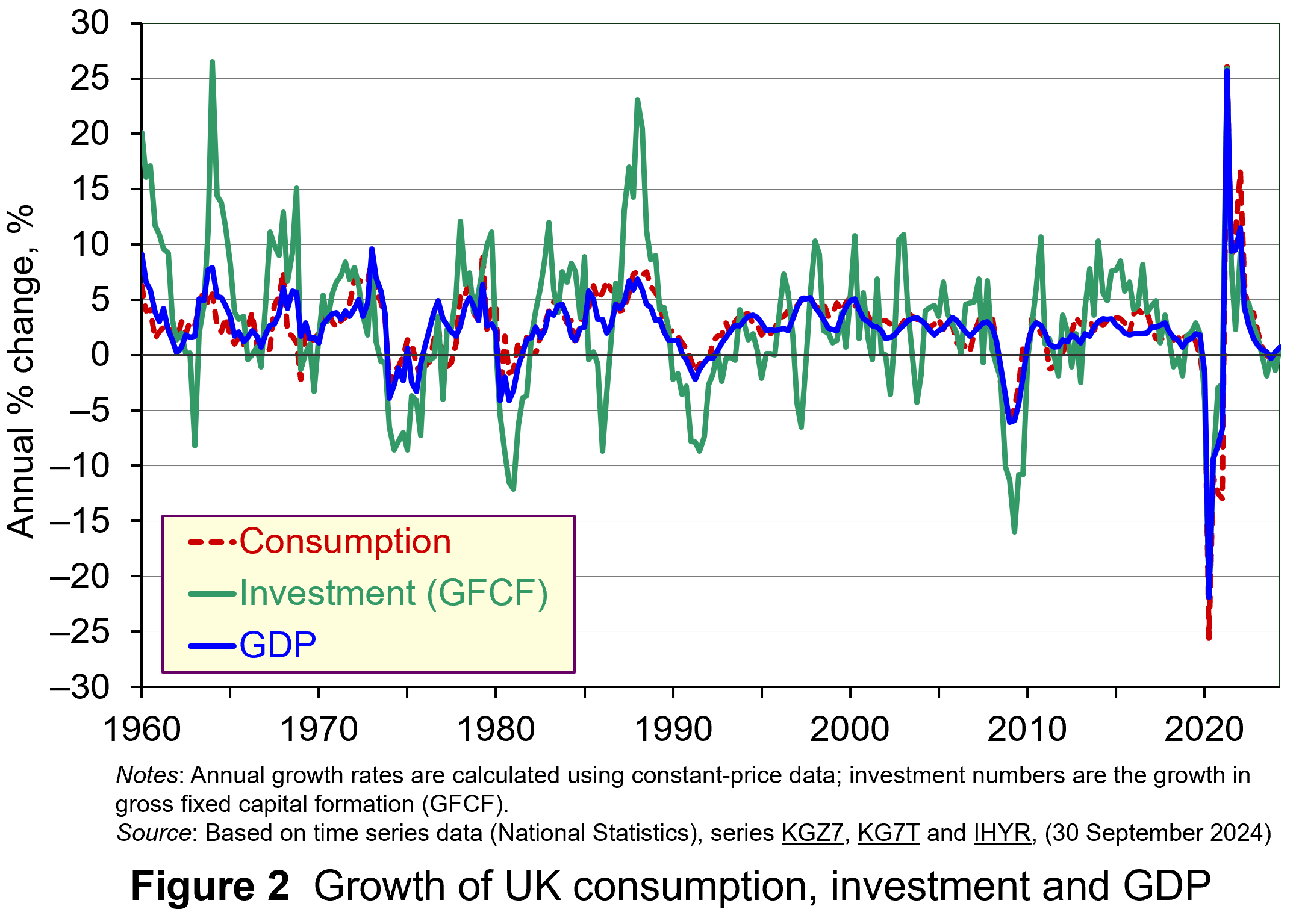 As Figure 2 shows (click here for a PowerPoint), investment is particularly volatile, and much more so than household spending. Some of this can be attributed to the ‘lumpiness’ of investment decisions since these expenditures tend to be characterised by indivisibility and irreversibility. This means that they are often relatively costly to finance and are ‘all or nothing’ decisions. In the context of uncertainty, it can make sense therefore for firms to wait for news that makes the future clearer. In this sense, we can think of uncertainty rather like a fog that firms are peering through. The thicker the fog, the more uncertain the future and the more cautious firms are likely to be.
The greater caution that many firms are likely to adopt in more uncertain times is consistent with the property of risk-aversion that we often attribute to a range of economic agents. When applied to household spending decisions, risk-aversion is often used to explain why households are willing to hold a buffer stock of savings to self-insure against unforeseen events and their future financial outcomes being worse than expected. Hence, in more uncertain times households are likely to want to increase this buffer further.
 The theory of buffer-stock saving was popularised by Christopher Carroll in 1992 (see link below). It implies that in the presence of uncertainty, people are prepared to consume less today in order to increase levels of saving, pay off existing debts, or borrow less relative to that in the absence of uncertainty. The extent of the buffer of financial wealth that people want to hold will depend on their own appetite for risk, the level of uncertainty, and the moderating effect from their own impatience and, hence, present bias for consuming today.
Risk aversion is consistent with the property of diminishing marginal utility of income or consumption. In other words, as people’s total spending volumes increase, their levels of utility or satisfaction increase but at an increasingly slower rate. It is this which explains why individuals are willing to engage with the financial system to reallocate their expected life-time earnings and have a smoother consumption profile than would otherwise be the case from their fluctuating incomes.
Yet diminishing marginal utility not only explains consumption smoothing, but also why people are willing to engage with the financial system to have financial buffers as self-insurance. It explains why people save more or borrow less today than suggested by our base-line consumption smoothing model. It is the result of people’s greater dislike (and loss of utility) from their financial affairs being worse than expected than their like (and additional utility) from them being better than expected. This tendency is only likely to increase the more uncertain times are. The result is that uncertainty tends to lower household consumption with perhaps ‘big-ticket items’, such as cars, furniture, and expensive electronic goods, being particularly sensitive to uncertainty.
Uncertainty and confidence
Uncertainty does not just affect risk; it also affects confidence. Risk and confidence are often considered together, not least because their effects in generating and transmitting shocks can be difficult to disentangle.
We can think of confidence as capturing our mood or sentiment, particularly with respect to future economic developments. Figure 3 plots the Uncertainty Index for the UK alongside the OECD’s composite consumer and business confidence indicators. Values above 100 for the confidence indicators indicate greater confidence about the future economic situation and near-term business environment, while values below 100 indicate pessimism towards the future economic and business environments.
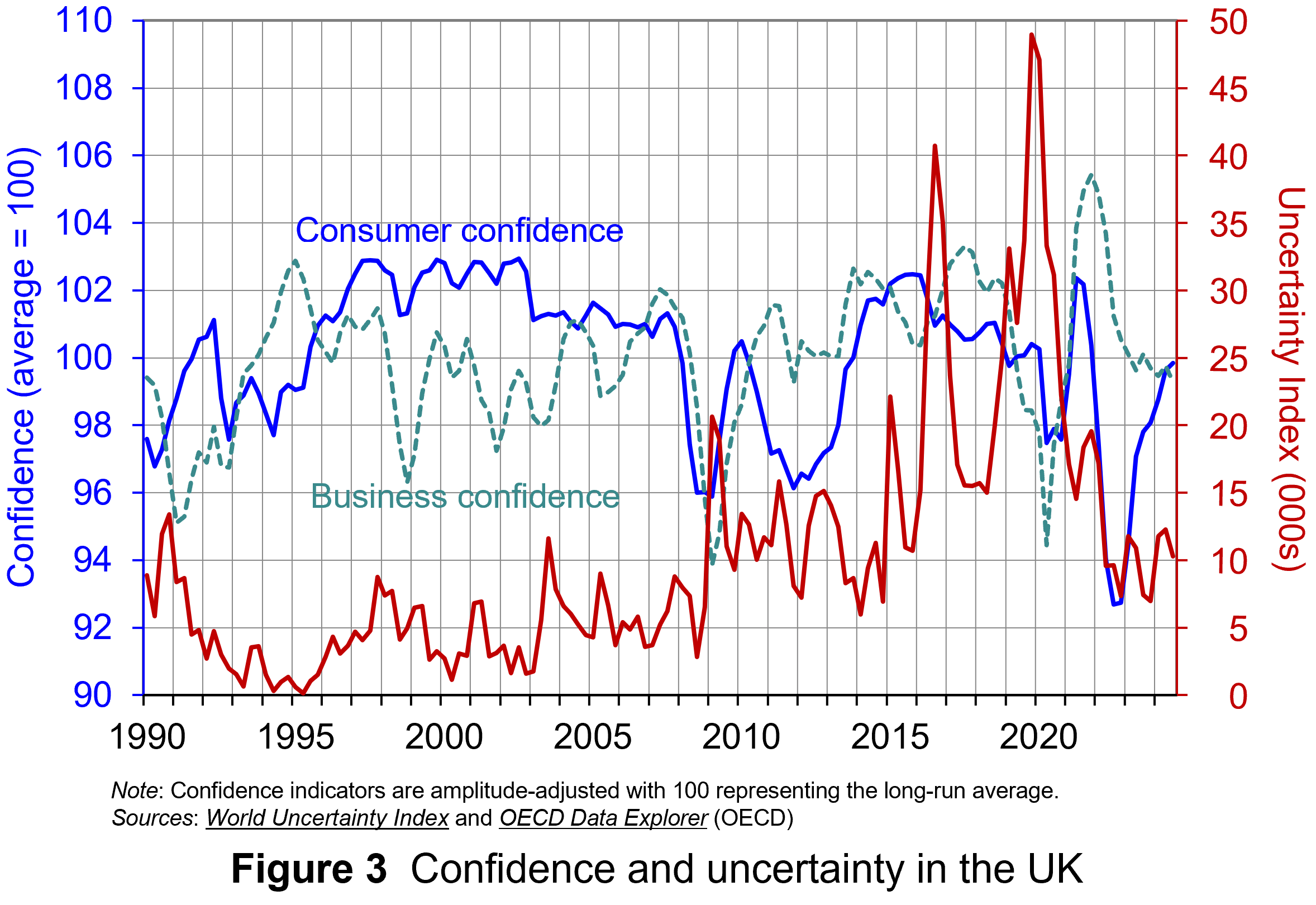 Figure 3 suggests that the relationship between confidence and uncertainty is rather more complex than perhaps is generally understood (click here for a PowerPoint). Haddow, Hare, Hooley and Shakir (see link below) argue that the evidence tends to point to changes in uncertainty affecting confidence, but with less evidence that changes in confidence affect uncertainty.
To illustrate this, consider the global financial crisis of the late 2000s. The argument can be made that the heightened uncertainty about future prospects for households and businesses helped to erode their confidence in the future. The result was that people and businesses revised down their expectations of the future (pessimism). However, although people were more pessimistic about the future, this was more likely to have been the result of uncertainty rather than the cause of further uncertainty.
Conclusion
For economists and policymakers alike, indicators of uncertainty, such as the Ahir, Bloom and Furceri World Uncertainty Index, are invaluable tools in understanding and forecasting behaviour and the likely economic outcomes that follow. Some uncertainty is inevitable, but the persistence of greater uncertainty since the global financial crisis of the late 2000s compares quite starkly with the relatively lower and more stable levels of uncertainty seen from the mid-1990s up to the crisis. Hence the recent frequency and size of changes in uncertainty show how important it to understand how uncertainty effects transmit through economies.
Academic papers
- The World Uncertainty Index
National Bureau of Economic Research, Working Paper 29763, Hites Ahir, Nicholas Bloom and Davide Furceri (February 2022)
- The Buffer-Stock Theory of Saving: Some Macroeconomic Evidence
Brookings Papers on Economic Activity, Christopher D Carroll (Vol 2, 1992)
- Macroeconomic uncertainty: what is it, how can we measure it and why does it matter?
Bank of England Quarterly Bulletin, 2013 Q2, Abigail Haddow, Chris Hare, John Hooley and Tamarah Shakir (13/6/13)
Articles
Data
Questions
- (a) Explain what is meant by the concept of diminishing marginal utility of consumption.
(b) Explain how this concept helps us to understand both consumption smoothing and the motivation to engage in buffer-stock saving.
- Explain the distinction between confidence and uncertainty when analysing macroeconomic shocks.
- Discuss which types of expenditures you think are likely to be most susceptible to uncertainty shocks.
- Discuss how economic uncertainty might affect productivity and the growth of potential output.
- How might the interconnectedness of economies affect the transmission of uncertainty effects through economies?
 In recent months there has been growing uncertainty across the global economy as to whether the US economy was going to experience a ‘hard’ or ‘soft landing’ in the current business cycle – the repeated sequences of expansion and contraction in economic activity over time. Announcements of macroeconomic indicators have been keenly anticipated for signals about how quickly the US economy is slowing.
Such heightened uncertainty is a common feature of late-cycle slowing economies, but uncertainty now has been exacerbated because it has been a while since developed economies have experienced a business cycle like the current one. The 21st century has been characterised by low inflation, low interest rates and recessions caused by various types of crises – a stock market crisis (2001), a banking crisis (2008) and a global pandemic (2020). In contrast, the current cycle is a throwback to the 20th century. The high inflation and the ensuing increases in interest rates have produced a business cycle which echoes the 1970s. Therefore, few investors have experience of such economic conditions.
The focus for investors during this stage of the cycle is when the slowing economy will reach the minimum. They will also be concerned with the depth of the slowdown: will there still be some growth in income, albeit low; or will the trough be severe enough to produce a recession, and, if so, how deep? Given uncertainty around the length and magnitude of business cycles, this leads to greater risk aversion among investors. This affects reactions to announcements of leading and lagging macroeconomic indicators.
This blog examines what sort of economic conditions we should expect in a late-cycle economy. It analyses the impact this has had on investor behaviour and the ensuing dynamics observed in financial markets in the USA.
The Business Cycle
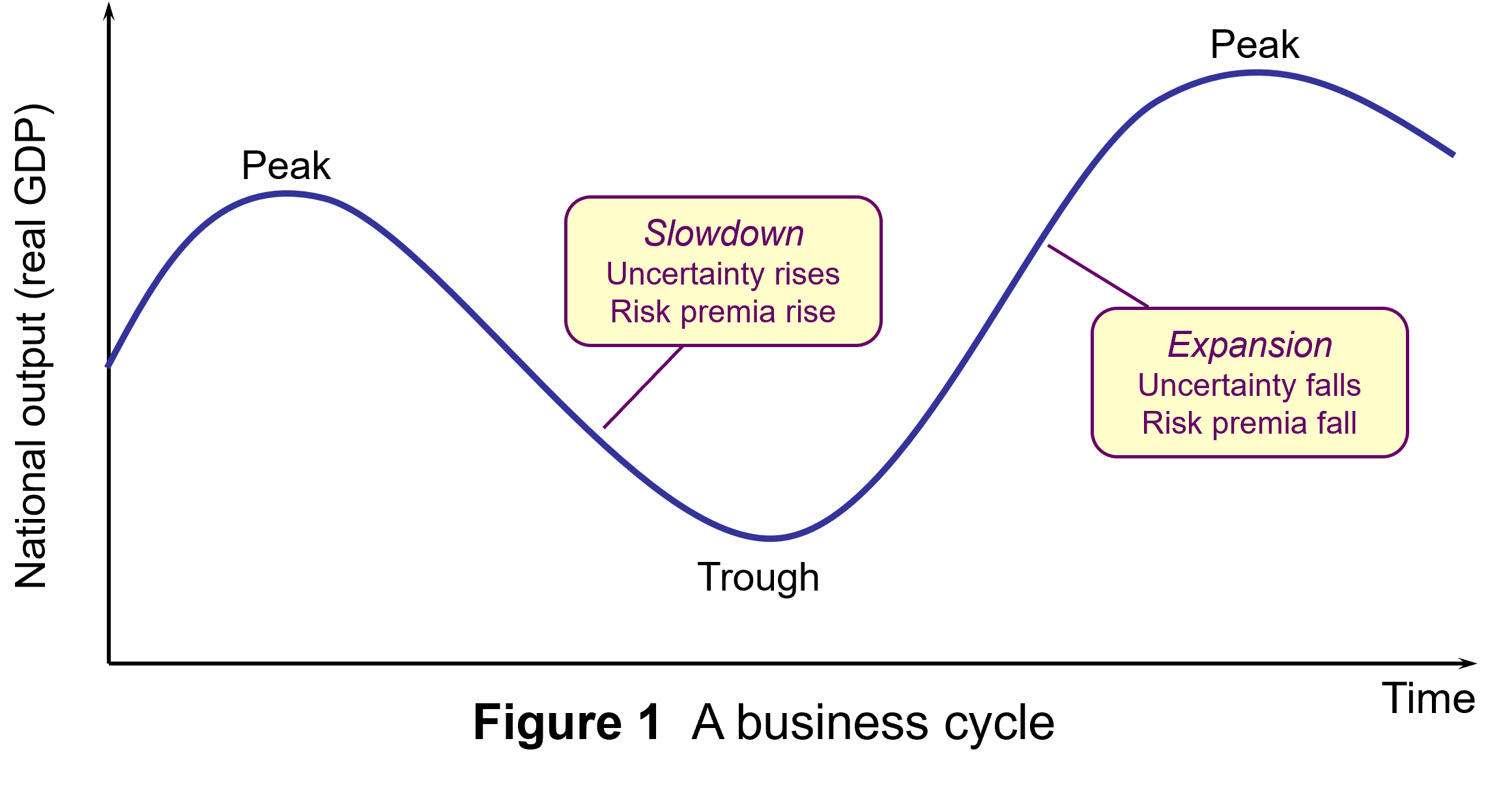
The business cycle refers to repeated sequences of expansion and contraction (or slowdown) in economic activity over time. Figure 1 illustrates a typical cycle. Typically, these sequences include four main stages. In each one there are different effects on consumer and business confidence:
- Expansion: During this stage, the economy experiences growth in GDP, with incomes and consumption spending rising. Business and consumer confidence are high. Unemployment is falling.
- Peak: This is the point at which the economy reaches its maximum output, but growth has ceased (or slowed). At this stage, inflationary pressures peak as the economy presses against potential output. This tends to result in tighter monetary policy (higher interest rates).
- Slowdown: The higher interest rates raise the cost of borrowing and reduce consumption and investment spending. Consumption and incomes both slow or fall. (Figure 1 illustrates the severe case of falling GDP (negative growth) in this stage.) Unemployment starts rising.
- Trough: This is the lowest point of the cycle, where economic activity bottoms out and the economy begins to recover. This can be associated with slow but still rising national income (a soft landing) or national income that has fallen (a hard landing, as shown in Figure 1).
While business cycles are common enough to enable such characterisation of their temporal pattern, their length and magnitude are variable and this produces great uncertainty, particularly when cycles approach peaks and troughs.
 As an economy’s cycle approaches a trough, such as US economy’s over the past few months, uncertainty is exacerbated. The high interest rates used to tackle inflation will have increased borrowing costs for businesses and consumers. Access to credit may have become more restricted. Profit margins are reduced, especially for industrial sectors sensitive to the business cycle, reducing expected cash flows.
The combination of these factors can increase the risk of a recession, producing greater volatility in financial markets. This manifests itself in increased risk aversion among investors.
Utility theory suggests that, in general, investors will exhibit loss aversion. This means that they do not like bearing risk, fearing that the return from an investment may be less than expected. In such circumstances, investors need to be compensated for bearing risk. This is normally expressed in terms of expected financial return. To bear more risk, investors require higher levels of return as compensation.
As perceptions of risk change through the business cycle, so this will change the return investors will require from the financial instruments they hold. Perceived higher risk raises the return investors will require as compensation. Conversely, lower perceived risk decreases the return investors expect as compensation.
Investors’ expected rate of return is manifested in the discount rate that they use to value the anticipated cash flows from financial instruments in discounted cash flow (DCF) analysis. Equation 1 is the algebraic expression of the present-value discounted series of cash flows for financial instruments:

Where:
V = present value
C = anticipated cash flows in each of time periods 1, 2, 3, etc.
r = expected rate of return
For fixed-income debt securities, the cash flow is constant, while for equity securities (shares), expectations regarding cash flows can change.
Slowing economies and risk aversion
 In a slowing economy, with great uncertainty about the scale and timing of the bottom of the cycle, investors become more risk averse about the prospects of firms. This this leads to higher risk premia for financial instruments sensitive to a slowdown in economic activity.
This translates into a higher expected return and higher discount rate used in the valuation of these instruments (r in equation 1). This produces decreases in perceived value, decreased demand and decreased prices for these financial instruments. This can be observed in the market dynamics for these instruments.
First, there may be a ‘flight to safety’. Investors attach a higher risk premium to risker financial instruments, such as equities, and seek a ‘safe-haven’ for their wealth. Therefore, we should observe a reorientation from more risky to less risky assets. Demand for equities falls, while demand for safer assets, such as government bonds and gold, rises.
There is some evidence for this behaviour as uncertainty about the US economic outlook has increased. Gold, long seen as a hedge against market decline, is at record highs. US Government bond prices have risen too.
To analyse whether this may be a flight to safety, I analysed the correlation between the daily US government bond price (5-year Treasury Bill) and share prices represented by the two more significant stock market indices in the USA: the S&P 500 and the Nasdaq Composite. I did this for two different time periods. Table 1 shows the results. Panel (a) shows the correlation coefficients for the period between 1 May 2024 and 31 July 2024; Panel (b) shows the correlation coefficients for the period between 1 August 2024 and 9 September 2024.
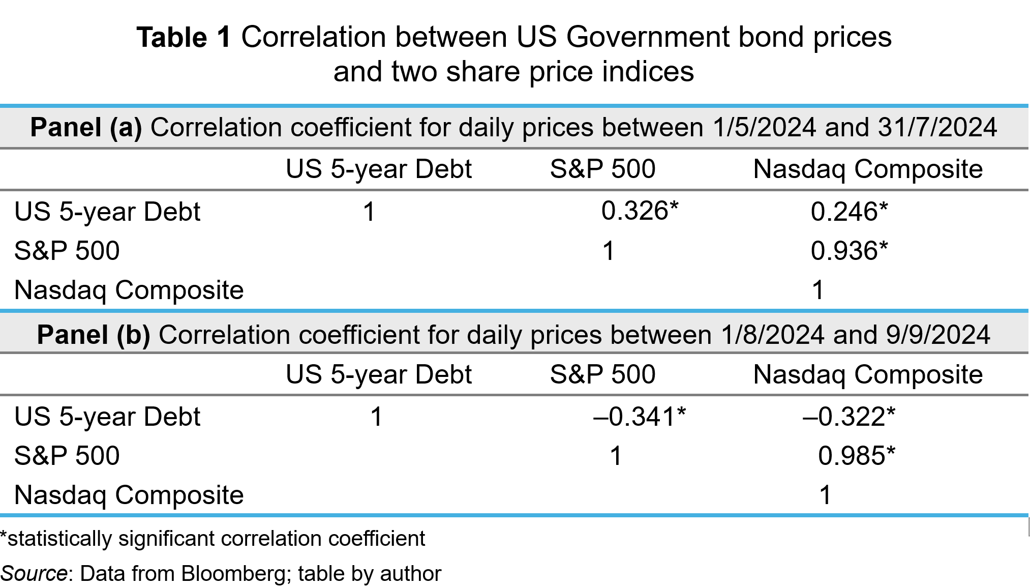
In the period between May and July 2024, the 5-year Treasury Bill and share price indices had significantly positive correlations. When share prices rose, the Treasury Bill’s price rose; when share prices fell, the bill’s price fell. During that period, expectations about falling interest rates dominated valuations and that effected the valuations of all financial instruments in the same way – lower expected interest rates reduce the opportunity cost of holding instruments and reduces the expected rates of return. Hence, the discount rate applied to cash flows is reduced, and present value rises. The opposite happens when macroeconomic indicators suggest that interest rates will stay high (ceteris paribus).
As the summer proceeded, worries about a ‘hard landing’ began to concern investors. A weak jobs report in early August particularly exercised markets, producing a ‘flight to safety’. Greater risk aversion among investors meant that they expect a higher return from equities. This reduced perceived value, reducing demand and price (ceteris paribus). To insulate themselves from higher risk, investors bought safer assets, like government bonds, thereby pushing up their prices. This behaviour was consistent with the significant negative correlation observed between US government debt prices and the S&P 500 and Nasdaq indices in Panel (b).
Another signal of increased risk aversion among investors is ‘sector rotation’ in their equity portfolios. Increased risk aversion among investors will lead them to divest from ‘cyclical’ companies. Such companies are in industrial sectors which are more sensitive to the changing economic conditions across the business cycle – consumer discretionary and communication services sectors, for example. To reduce their exposure to risk, investors will switch to ‘defensive’ sectors – those less sensitive to the business cycle. Examples include consumer staples and utility sectors.
Cyclical sectors will suffer a greater adverse impact on their cash flows and risk in a slowing economy. Consequently, investors expect higher return as compensation. This reduces the value of those shares. Demand for them falls, depressing their price. In contrast, defensive sectors will be valued more. They will see an increase in demand and price. This sector rotation seems to have happened in August (2024). Figure 2 shows the percentage change between 1 August and 9 September 2024 in the S&P 500 index and four sector indices, comprising companies from the communication services, consumer discretionary, consumer staples and utilities sectors.
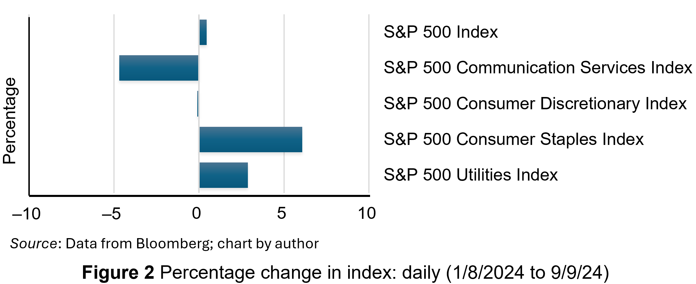
Overall, the S&P 500 index was slightly higher, as shown by the first bar in the chart. However, while the cyclical sectors experienced decreases in their share prices, particularly communication services, the defensive companies experienced large price increases – nearly 3% for utilities and over 6% for consumer staples.
Conclusion
Economies experience repeated sequences of expansion and contraction in economic activity over time. At the moment, the US economy is approaching the end of its current slowing phase. Increased uncertainty is a common feature of late-cycle economies and this manifests itself in heightened risk aversion among investors. This produces certain dynamics which have been observable in US debt and equity markets. This includes a ‘flight to safety’, with investors divesting risky financial instruments in favour of safer ones, such as US government debt securities and gold. Also, investors have been reorientating their equity portfolios away from cyclicals and towards defensive securities.
Articles
- America’s recession signals are flashing red. Don’t believe them
The Economist (22/8/24)
- The most well-known recession indicator stopped flashing red, but now another one is going off
CNN, Elisabeth Buchwald (13/9/24)
- World’s largest economy will still achieve soft landing despite rising unemployment, most analysts believe
Financial Times, Claire Jones, Delphine Strauss and Martha Muir (6/8/24)
- We’re officially on slowdown watch
Financial Times, Robert Armstrong and Aiden Reiter (30/8/24)
- Anatomy of a rout
Financial Times, Robert Armstrong and Aiden Reiter (6/8/24)
- Reasons why investors need to prepare for a US recession
Financial Times, Peter Berezin (5/9/24)
- Business Cycle: What It Is, How to Measure It, and Its 4 Phases
Investopedia, Lakshman Achuthan (6/6/24)
- Risk Averse: What It Means, Investment Choices, and Strategies
Investopedia, James Chen (5/8/24)
Data
Questions
- What is risk aversion? Sketch an indifference curve for a risk-averse investor, treating expected return and risk as two-characteristics of a financial instrument.
- Show what happens to the slope of the indifference curve if the investor becomes more risk averse.
- Using demand and supply analysis, illustrate and explain the impact of a flight to safety on the market for (i) company shares and (ii) US government Treasury Bills.
- Use economic theory to explain why the consumer discretionary sector may be more sensitive than the consumer staples sector to varying incomes across the economic cycle.
- Research the point of the economic cycle that the US economy has reached as you read this blog. What is the relationship between bond and equity prices? Which sectors have performed best in the stock market?
 Global long-term economic growth has slowed dramatically since the financial crisis of 2007–8. This can be illustrated by comparing the two 20-year periods 1988 to 2007 and 2009 to 2028 (where IMF forecasts are used for 2024 to 2028: see WEO Database under the Data link below). Over the two periods, average annual world growth fell from 3.8% to 3.1%. In advanced countries it fell from 2.9% to 1.6% and in developing countries from 4.8% to 4.3%. In the UK it fell from 2.4% to 1.2%, in the USA from 3.1% to 1.8% and in Japan from 1.9% to 0.5%.
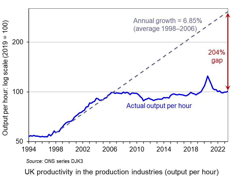 In the UK, labour productivity growth in the production industries was 6.85% per annum from 1998 to 2006. If this growth rate had been maintained, productivity would have been 204% higher by the end of 2023 than it actually was. This is shown in the chart (click here for a PowerPoint).
The key driver of long-term economic growth is labour productivity, which can best be measured by real GDP per hour worked. This depends on three things: the amount of capital per worker, the productivity of this capital and the efficiency of workers themselves – the latter two giving total factor productivity (TFP). Productivity growth has slowed, and with it the long-term rate of economic growth.
If we are measuring growth in output per head of the population, as opposed to simple growth in output, then another important factor is the proportion of the population that works. With ageing populations, many countries are facing an increase in the proportion of people not working. In most countries, these demographic pressures are likely to increase.
 A major determinant of long-term economic growth and productivity is investment. Investment has been badly affected by crises, such as the financial crisis and COVID, and by geopolitical tensions, such as the war in Ukraine and tensions between the USA and China and potential trade wars. It has also been adversely affected by government attempts to deal with rising debt caused by interventions following the financial crisis and COVID. The fiscal squeeze and, more recently higher interest rates, have dampened short-term growth and discouraged investment, thereby dampening long-term growth.
Another factor adversely affecting productivity has been a lower growth of allocative efficiency. Competition in many industries has declined as the rate of new firms entering and exiting markets has slowed. The result has been an increase in concentration and a growth in supernormal profits.
In the UK’s case, growth prospects have also been damaged by Brexit. According to Bank of England and OBR estimates, Brexit has reduced productivity by around 4% (see the blog: The costs of Brexit: a clearer picture). For many companies in the UK, Brexit has hugely increased the administrative burdens of trading with the EU. It has also reduced investment and led to a slower growth in the capital stock.
The UK’s poor productivity growth over many yeas is examined in the blog The UK’s poor productivity record.
Boosting productivity
So, how could productivity be increased and what policies could help the process?
 Artificial intelligence. One important driver of productivity growth is technological advance. The rapid advance in AI and its adoption across much of industry is likely to have a dramatic effect on working practices and output. Estimates by the IMF suggest that some 40% of jobs globally and 60% in advanced countries could be affected – some replaced and others complemented and enhanced by AI. The opportunities for raising incomes are huge, but so too are the dangers of displacing workers and deepening inequality, as some higher-paid jobs are enhanced by AI, while many lower paid jobs are little affected and other jobs disappear.
AI is also likely to increase returns to capital. This may help to drive investment and further boost economic growth. However, the increased returns to capital are also likely to exacerbate inequality.
To guard against the growth of market power and its abuse, competition policies may need strengthening to ensure that the benefits of AI are widely spread and that new entrants are encouraged. Also training and retraining opportunities to allow workers to embrace AI and increase their mobility will need to be provided.
 Training. And it is not just training in the use of AI that is important. Training generally is a key ingredient in encouraging productivity growth. In the UK, there has been a decline in investment in adult education and training, with a 70% reduction since the early 2000s in the number of adults undertaking publicly-funded training, and with average spending on training by employers decreasing by 27% per trainee since 2011. The Institute for Fiscal Studies identifies five main policy levers to address this: “public funding of qualifications and skills programmes, loans to learners, training subsidies, taxation of training and the regulation of training” (see link in articles below).
Competition. Another factor likely to enhance productivity is competition, both internationally and within countries. Removing trade restrictions could boost productivity growth; erecting barriers to protect inefficient domestic industry would reduce it.
Investment. Policies to encourage investment are also key to productivity growth. Private-sector investment can be encouraged by tax incentives. For example, in the UK the Annual Investment Allowance allows businesses to claim 100% of the cost of plant and machinery up to £1m in the year it is incurred. However, for tax relief to produce significant effects on investment, companies need to believe that the policy will stay and not be changed as economic circumstances or governments change.
 Public-sector investment is also key. Good road and rail infrastructure and public transport are vital in encouraging private investment and labour mobility. And investment in health, education and training are a key part in encouraging the development of human capital. Many countries, the UK included, cut back on public-sector capital investment after the financial crisis and this has had a dampening effect on economic growth.
Regional policy. External economies of scale could be encouraged by setting up development areas in various regions. Particular industries could be attracted to specific areas, where local skilled workers, managerial expertise and shared infrastructure can benefit all the firms in the industry. These ‘agglomeration economies’ have been very limited in the UK compared with many other countries with much stronger regional economies.
Changing the aims and governance of firms. A change in corporate structure and governance could also help to drive investment and productivity. According to research by the think tank, Demos (see the B Lab UK article and the second report below), if legislation required companies to consider the social, economic and environmental impact of their business alongside profitability, this could have a dramatic effect on productivity. If businesses were required to be ‘purpose-led’, considering the interests of all their stakeholders, this supply-side reform could dramatically increase growth and well-being.
Such stakeholder-governed businesses currently outperform their peers with higher levels of investment, innovation, product development and output. They also have higher levels of staff engagement and satisfaction.
Articles
- World Must Prioritize Productivity Reforms to Revive Medium-Term Growth
IMF Blog, Nan Li and Diaa Noureldin (10/4/24)
- Why has productivity slowed down?
Oxford Martin School News, Ian Goldin, Pantelis Koutroumpis, François Lafond and Julian Winkler (18/3/24)
- How can the UK revive its ailing productivity?
Economics Observatory, Michelle Kilfoyle (14/3/24)
- With the UK creeping out of recession, here’s an economist’s brief guide to improving productivity
The Conversation, Nigel Driffield (13/3/24)
- UK economy nearly a third smaller thanks to ‘catastrophically bad’ productivity slowdown
City A.M., Chris Dorrell (12/3/24)
- Can AI help solve the UK’s public sector productivity puzzle?
City A.M., Chris Dorrell (11/3/24)
- AI Will Transform the Global Economy. Let’s Make Sure it Benefits Humanity
IMF Blog, Kristalina Georgieva (14/1/24)
- Productivity and Investment: Time to Manage the Project of Renewal
NIESR, Paul Fisher (12/3/24)
- Productivity trends using key national accounts indicators
Eurostat (15/3/24)
- New report says change to company law could add £149bn to the UK economy
B Lab UK (28/11/23)
- Investment in training and skills: Green Budget Chapter 9
Institute for Fiscal Studies, Imran Tahir (12/10/23)
Reports
Data
Questions
- Why has global productivity growth been lower since 2008 than before 2008?
- Why has the UK’s productivity growth been lower than many other advanced economies?
- How does the short-run macroeconomic environment affect long-term growth?
- Find out why Japan’s productivity growth has been so poor compared with other countries.
- What are likely to be the most effective means of increasing productivity growth?
- How may demand management policies affect the supply side of the economy?
- How may the adoption of an ESG framework by companies for setting objectives affect productivity growth?
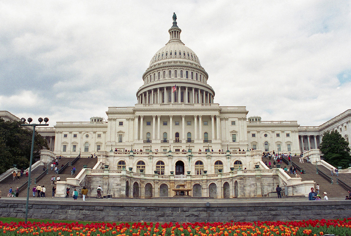 On 10 March, the House of Representatives gave final approval to President Biden’s $1.9tr fiscal stimulus plan (the American Rescue Plan). Worth over 9% of GDP, this represents the third stage of an unparalleled boost to the US economy. In March 2020, President Trump secured congressional agreement for a $2.2tr package (the CARES Act). Then in December 2020, a bipartisan COVID relief bill, worth $902bn, was passed by Congress.
By comparison, the Obama package in 2009 in response to the impending recession following the financial crisis was $831bn (5.7% of GDP).
The American Rescue Plan
The Biden stimulus programme consists of a range of measures, the majority of which provide monetary support to individuals. These include a payment of $1400 per person for single people earning less than $75 000 and couples less than $150 000. These come on top of payments of $1200 in March 2020 and $600 in late December. In addition, the top-up to unemployment benefits of $300 per week agreed in December will now continue until September. Also, annual child tax credit will rise from $2000 annually to as much as $3600 and this benefit will be available in advance.
 Other measures include $350bn in grants for local governments depending on their levels of unemployment and other needs; $50bn to improve COVID testing centres and $20bn to develop a national vaccination campaign; $170bn to schools and universities to help them reopen after lockdown; and grants to small businesses and specific grants to hard-hit sectors, such as hospitality, airlines, airports and rail companies.
Despite supporting the two earlier packages, no Republican representative or senator backed this latest package, arguing that it was not sufficiently focused. As a result, reaction to the package has been very much along partisan lines. Nevertheless, it is supported by some 90% of Democrat voters and 50% of Republican voters.
Is the stimulus the right amount?
Although the latest package is worth $1.9tr, aggregate demand will not expand by this amount, which will limit the size of the multiplier effect. The reason is that the benefits multiplier is less than the government expenditure multiplier as some of the extra money people receive will be saved or used to reduce debts.
With $3tr representing some 9% of GDP, this should easily fill the estimated negative output gap of between 2% and 3%, especially when multiplier effects are included. Also, with savings having increased during the recession to put them some 7% above normal, the additional amount saved may be quite small, and wealthier Americans may begin to reduce their savings and spend a larger proportion of their income.
 So the problem might be one of excessive stimulus, which in normal times could result in crowding out by driving up interest rates and dampening investment. However, the Fed is still engaged in a programme of quantitative easing. Between mid-March 2020 and the end of March 2021, the Fed’s portfolio of securities held outright grew from $3.9tr to $7.2tr. What is more, many economists predict that inflation is unlikely to rise other than very slightly. If this is so, it should allow the package to be financed easily. Debt should not rise to unsustainable levels.
Other economists argue, however, that inflationary expectations are rising, reflected in bond yields, and this could drive actual inflation and force the Fed into the awkward dilemma of either raising interest rates, which could have a significant dampening effect, or further increasing money supply, potentially leading to greater inflationary problems in the future.
A lot will depend what happens to potential GDP. Will it rise over the medium term so that additional spending can be accommodated? If the rise in spending encourages an increase in investment, this should increase potential GDP. This will depend on business confidence, which may be boosted by the package or may be dampened by worries about inflation.
Additional packages to come
 Potential GDP should also be boosted by two further packages that Biden plans to put to Congress.
The first is a $2.2tr infrastructure investment plan, known as the American Jobs Plan. This is a 10-year plan to invest public money in transport infrastructure (such as rebuilding 20 000 miles of road and repairing bridges), public transport, electric vehicles, green housing, schools, water supply, green power generation, modernising the power grid, broadband, R&D in fields such as AI, social care, job training and manufacturing. This will be largely funded through tax increases, such as gradually raising corporation tax from 21% to 28% (it had been cut from 35% to 21% by President Trump) and taxing global profits of US multinationals. However, the spending will generally precede the increased revenues and thus will raise aggregate demand in the initial years. Only after 15 years are revenues expected to exceed costs.
The second is a yet-to-be announced plan to increase spending on childcare, healthcare and education. This should be worth at least $1tr. This will probably be funded by tax increases on income, capital gains and property, aimed largely at wealthy individuals. Again, it is hoped that this will boost potential GDP, in this case by increasing labour productivity.
With earlier packages, the total increase in public spending will be over $8tr. This is discretionary fiscal policy writ large.
Articles
- Biden’s $1.9 trillion COVID-19 bill wins final approval in House
Reuters, Susan Cornwell and Makini Brice (10/3/21)
- Biden’s Covid stimulus plan: It costs $1.9tn but what’s in it?
BBC News, Natalie Sherman (6/3/21)
- Biden’s $1.9 Trillion Challenge: End the Coronavirus Crisis Faster
New York Times, Jim Tankersley and Sheryl Gay Stolberg (22/3/21)
- Joe Biden writes a cheque for America – and the rest of the world
The Observer, Phillip Inman (13/3/21)
- Spend or save: Will Biden’s stimulus cheques boost the economy?
Aljazeera, Cinnamon Janzer (9/3/21)
- After Biden stimulus, US economic growth could rival China’s for the first time in decades
CNN, Matt Egan (12/3/21)
- Larry Summers, who called out inflation fears with Biden’s $1.9 trillion COVID-19 relief package, says the US is seeing ‘least responsible’ macroeconomic policy in 40 years
Business Insider, John L. Dorman (21/3/21)
- With $1.9 Trillion in New Spending, America Is Headed for Financial Fragility
Barron’s, Leslie Lipschitz and Josh Felman (30/3/21)
- Biden unveils ‘once-in-a generation’ $2tn infrastructure investment plan
The Guardian, Lauren Gambino (31/3/21)
- Biden unveils $2tn infrastructure plan and big corporate tax rise
Financial Times, James Politi (31/3/21)
- The Observer view on Joe Biden’s audacious spending plans
The Observer, editorial (11/4/21)
Videos
Questions
- Draw a Keynesian cross diagram to show the effect of an increase in benefits when the economy is operating below potential GDP.
- What determines the size of the benefits multiplier?
- Explain what is meant by the output gap. How might the pandemic and accompanying emergency health measures have affected the size of the output gap?
- How are expectations relevant to the effectiveness of the stimulus measures?
- What is likely to determine the proportion of the $1400 stimulus cheques that people spend?
- Distinguish between resource crowding out and financial crowding out. Is the fiscal stimulus package likely to result in either form of crowding out and, if so, what will determine by how much?
- What is the current monetary policy of the Fed? How is it likely to impact on the effectiveness of the fiscal stimulus?
 Economic growth is closely linked to investment. In the short term, there is a demand-side effect: higher investment, by increasing aggregate demand, creates a multiplier effect. GDP rises and unemployment falls. Over the longer term, higher net investment causes a supply-side effect: industrial capacity and potential output rise. This will be from both the greater quantity of capital and, if new investment incorporates superior technology, from a greater productivity of capital.
 There is currently great uncertainty in the USA and its trading partners. The frequent changes in policy by President Trump are causing a fall in confidence and consequently a fall in investment. The past few weeks have seen large cuts in US government expenditure as his administration seeks to dismantle the current structure of government. The businesses supplying federal agencies thus face great uncertainty about future contracts. Laid-off workers will be forced to cut their spending, which will have knock-on effect on business, who will cut employment and investment as the multiplier and accelerator work through.
 Perhaps the biggest uncertainty for business concerns the imposition of tariffs. Many US businesses rely on imports of raw materials, components, equipment, etc. Imposing tariffs on imports raises business costs. But this will vary from firm to firm, depending on the proportion of their inputs that are imported. And even when the inputs are from other US companies, those companies may rely on imports and thus be forced to raise prices to their customers. And if, in retaliation, other countries impose tariffs on US goods, this will affect US exporters and discourage them from investing.
 Trump An ‘Uncertainty Tax’ Says Vanguard Chief Economist
 This week in Trumponomics: Playing chicken with markets
 We continue to live through incredibly turbulent times. In the past decade or so we have experienced a global financial crisis, a global health emergency, seen the UK’s departure from the European Union, and witnessed increasing levels of geopolitical tension and conflict. Add to this the effects from the climate emergency and it easy to see why the issue of economic uncertainty is so important when thinking about a country’s economic prospects.
 Figure 1 (click
  As Figure 2 shows (click
  The theory of buffer-stock saving was popularised by Christopher Carroll in 1992 (see link below). It implies that in the presence of uncertainty, people are prepared to consume less today in order to increase levels of saving, pay off existing debts, or borrow less relative to that in the absence of uncertainty. The extent of the buffer of financial wealth that people want to hold will depend on their own appetite for risk, the level of uncertainty, and the moderating effect from their own impatience and, hence, present bias for consuming today.
 Figure 3 suggests that the relationship between confidence and uncertainty is rather more complex than perhaps is generally understood (click
 As an economy’s cycle approaches a trough, such as US economy’s over the past few months, uncertainty is exacerbated. The high interest rates used to tackle inflation will have increased borrowing costs for businesses and consumers. Access to credit may have become more restricted. Profit margins are reduced, especially for industrial sectors sensitive to the business cycle, reducing expected cash flows.
 In a slowing economy, with great uncertainty about the scale and timing of the bottom of the cycle, investors become more risk averse about the prospects of firms. This this leads to higher risk premia for financial instruments sensitive to a slowdown in economic activity.

 Global long-term economic growth has slowed dramatically since the financial crisis of 2007–8. This can be illustrated by comparing the two 20-year periods 1988 to 2007 and 2009 to 2028 (where IMF forecasts are used for 2024 to 2028: see WEO Database under the Data link below). Over the two periods, average annual world growth fell from 3.8% to 3.1%. In advanced countries it fell from 2.9% to 1.6% and in developing countries from 4.8% to 4.3%. In the UK it fell from 2.4% to 1.2%, in the USA from 3.1% to 1.8% and in Japan from 1.9% to 0.5%.
 In the UK, labour productivity growth in the production industries was 6.85% per annum from 1998 to 2006. If this growth rate had been maintained, productivity would have been 204% higher by the end of 2023 than it actually was. This is shown in the chart (click
  A major determinant of long-term economic growth and productivity is investment. Investment has been badly affected by crises, such as the financial crisis and COVID, and by geopolitical tensions, such as the war in Ukraine and tensions between the USA and China and potential trade wars. It has also been adversely affected by government attempts to deal with rising debt caused by interventions following the financial crisis and COVID. The fiscal squeeze and, more recently higher interest rates, have dampened short-term growth and discouraged investment, thereby dampening long-term growth.
 Artificial intelligence. One important driver of productivity growth is technological advance. The rapid advance in AI and its adoption across much of industry is likely to have a dramatic effect on working practices and output.
  Training. And it is not just training in the use of AI that is important. Training generally is a key ingredient in encouraging productivity growth. In the UK, there has been a decline in investment in adult education and training, with a 70% reduction since the early 2000s in the number of adults undertaking publicly-funded training, and with average spending on training by employers decreasing by 27% per trainee since 2011. The Institute for Fiscal Studies identifies five main policy levers to address this: “public funding of qualifications and skills programmes, loans to learners, training subsidies, taxation of training and the regulation of training” (see link in articles below).
 Public-sector investment is also key. Good road and rail infrastructure and public transport are vital in encouraging private investment and labour mobility. And investment in health, education and training are a key part in encouraging the development of human capital. Many countries, the UK included, cut back on public-sector capital investment after the financial crisis and this has had a dampening effect on economic growth.
 On 10 March, the House of Representatives gave final approval to President Biden’s $1.9tr fiscal stimulus plan (the
  Other measures include $350bn in grants for local governments depending on their levels of unemployment and other needs; $50bn to improve COVID testing centres and $20bn to develop a national vaccination campaign; $170bn to schools and universities to help them reopen after lockdown; and grants to small businesses and specific grants to hard-hit sectors, such as hospitality, airlines, airports and rail companies.
 So the problem might be one of excessive stimulus, which in normal times could result in crowding out by driving up interest rates and dampening investment. However, the Fed is still engaged in a programme of quantitative easing. Between mid-March 2020 and the end of March 2021, the Fed’s
  Potential GDP should also be boosted by two further packages that Biden plans to put to Congress.