 In the second of a series of blogs looking at applications of the distinction between nominal and real indicators, we revisit the blog Getting Real with Growth last updated in October 2021.
In this blog, we discuss how, in making a meaningful comparison over time of a country’s national income and, therefore, the aggregate purchasing power of its people, we need to take inflation into account. Likewise, if we want to analyse changes in the volume of production, we need to eliminate the effects of price changes on GDP. This is important when analysing the business cycle and identifying periods of boom or bust. Hence, in this updated blog we take another look at what real GDP data reveal about both longer-term economic growth and the extent of economic volatility – or what we refer to as the twin characteristics of economic growth.
Real and nominal GDP
The nominal (or current-price) estimate for UK gross domestic product in 2023 was £2.687 trillion. The estimate of national output or national income is based primarily on the production of final goods and services and, hence, purchased by the final user. It therefore largely excludes intermediate goods and services: i.e. goods and services that are transformed or used up in the process of making something else, although data on imports and exports do include intermediate goods and services. The 2023 figure represents a nominal increase in national income of 7.2 per cent on the £2.51 trillion recorded in 2022. These values make no adjustment for inflation and therefore reflect the prices of output that were prevailing at the time.
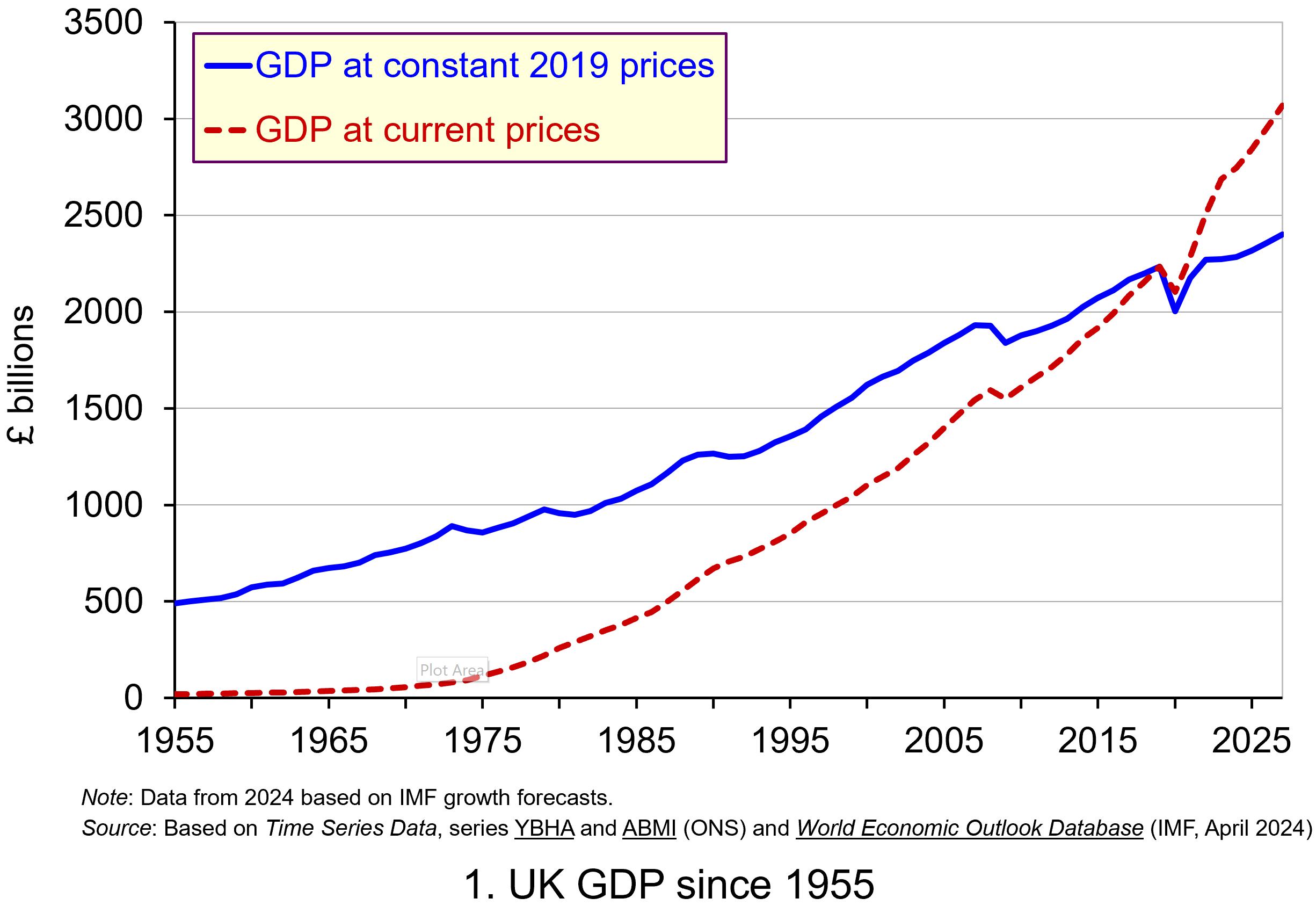 Chart 1 shows current-price estimates of GDP from 1955, when the value of GDP was estimated at £19.2 billion. The £2.687 trillion figure recorded for 2023 is an increase of over 140 times that in 1955, a figure that rises to 160 times if we compare the 1950 value with the latest IMF estimate for 2027. However, if we want to make a more meaningful comparison of the country’s national income we need to adjust for inflation. (Click here to download a PowerPoint of the chart.)
Long-term growth in real GDP
If we measure GDP at constant prices, we eliminate the effect of inflation. To construct a constant-price series for GDP, a process known as chain-linking is used. This involves taking consecutive pairs of years, e.g. 2022 and 2023, and estimating what GDP would be in the most recent year (in this case, 2023) if the previous year’s prices (i.e. 2022) had continued to prevail. By calculating the percentage change from the previous year’s GDP value we have an estimate of the volume change. If this is repeated for other pairs of years, we have a series of percentage changes that capture the volume changes from year-to-year. Finally, a reference year is chosen and the percentage volume changes are applied backwards and forwards from the nominal GDP value for the reference year.
In effect, a real GDP series creates a quantity measure in monetary terms. Chart 1 shows GDP at constant 2019 prices (real GDP) alongside GDP at current prices (nominal GDP). Consider first the real GDP numbers for 1955 and 2023. GDP in 1950 at 2019 prices was £491.2 billion. This is higher than the current-price value because prices in 2019 (the reference year) were higher than those in 1955. Meanwhile, GDP in 2023 when measured at 2019 prices was £2.273 trillion. This constant-price value is smaller than the corresponding current-price value because prices in 2019 where lower than those in 2023.
 Between 1955 and 2023 real GDP increased 4.6 times. If we extend the period to 2027, again using the latest IMF estimates, the increase is 4.9 times. Because we have removed the effect of inflation, the real growth figure is much lower than the nominal growth figure.
Crucially, what we are left with is an indicator of the long-term growth in the volume of the economy’s output and hence an increase in national income that is backed up by an increase in production. Whereas nominal growth rates are affected by changes in both volumes and prices, real growth rates reflect only changes in volumes.
The upward trajectory observed in constant-price GDP is therefore evidence of positive longer-term growth. This is one of the twin characteristics of growth.
Short-term fluctuations in the growth of real GDP
The second characteristic is fluctuations in the rate of growth from period to period. We can see this second characteristic more clearly by plotting the percentage change in real GDP from year to year.
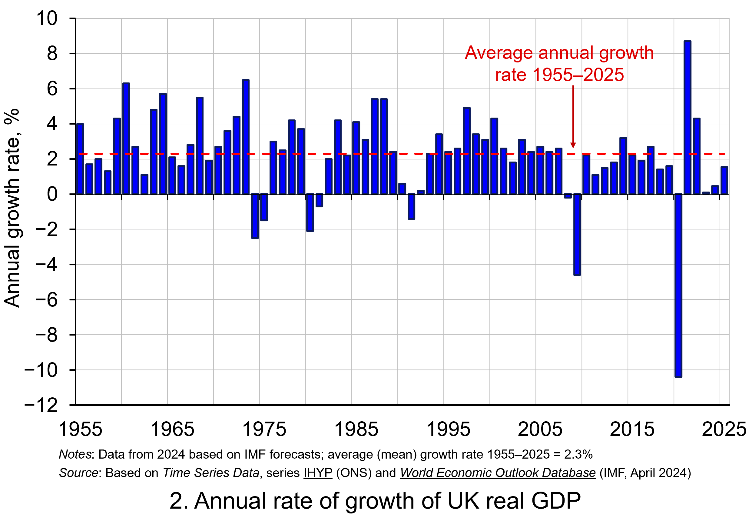 Chart 2 shows the annual rate of growth in real GDP each year from 1955 to 2025. From it, we see the inherent instability that is a key characteristic of the macroeconomic environment. This instability is, of course, mirrored in the output path of real GDP in Chart 1, but the annual rates of growth show the instability more clearly. We can readily see the impact on national output of the global financial crisis of 2007–8 and the global COVID pandemic.
In 2009, constant-price GDP in the UK fell by 4.6 per cent, whereas current-price GDP fell by 2.8 per cent. Then, in 2020, constant-price GDP and, hence, the volume of national output fell by 10.4 per cent, as compared to a 5.8 per cent fall in current-price GDP. These global, ‘once-in-a-generation’ shocks are stark examples of the instability that characterises economies and which generate the ‘ups and downs’ in an economy’s output path, known more simply as ‘the business cycle’. (Click here to download a PowerPoint copy of the chart.)
Determinants of long-and short-term growth
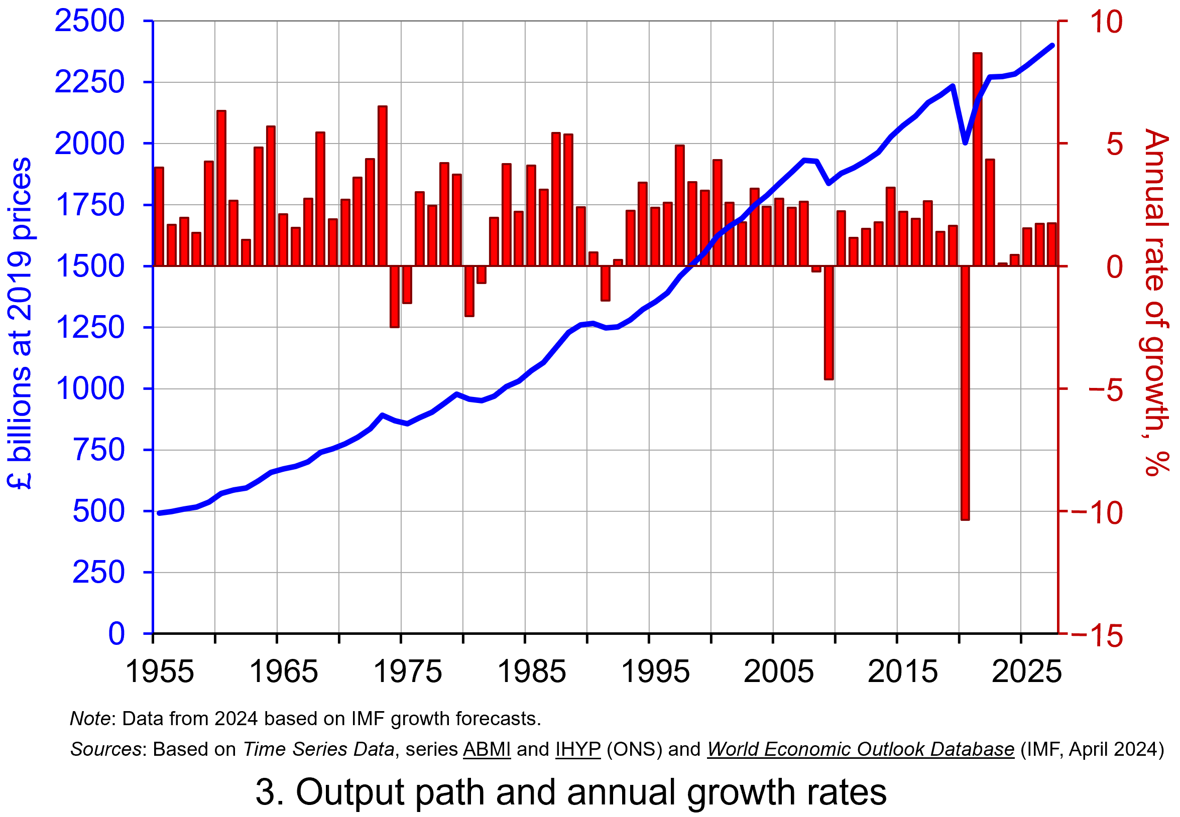 The twin characteristics of growth can be seen simultaneously by combining the output path (shown by the levels of real GDP) with the annual rates of growth. This is shown in Chart 3. The longer-term growth seen in the economy’s output path is generally argued to be driven by the quantity and quality of the economy’s resources, and their effectiveness when combined in production (i.e. their productivity). In other words, it is the supply side of the economy that determines the trajectory of the output path over the longer term. (Click here to download a PowerPoint copy of the chart.)
However, the fluctuations we observe in short-term growth rates tend to reflect shocks, also known as impulses, that originate either from the ability and or willingness of purchasers to consume (demand-side shocks) or producers to supply (supply-side shocks). These impulses are then amplified (or ‘propagated’) via the multiplier, expectations and other factors, and their effects, therefore, transmitted through the economy. Unusually in the case of the pandemic, the lockdown measures employed by governments around the world resulted in simultaneous negative aggregate demand and aggregate supply shocks.
Persistence effects
Explanations of the business cycle and of long-term growth are not mutually exclusive. The shocks and the propagation mechanisms that help to create and shape the business cycle can themselves have enduring or persistent effects on output. The global financial crisis, fuelled by unsustainable lending and the overstretch of private-sector balance sheets, which then spilt over to the public sector as governments attempted to stabilise the financial system and support aggregate demand, is argued by some to have created the conditions for low-growth persistence seen in many countries in the 2010s. This type of persistence is known as hysteresis as it originates from a negative demand shock.
Economists and policymakers were similarly concerned that the pandemic would also generate persistence in the form of scarring effects that might again affect the economy’s output path. Such concerns help to explain why many governments introduced furlough schemes to protect jobs and employment income, as well as provide grants or loans to business.
Per capita output
To finish, it is important to recognise that, when thinking about living standards, it is the growth in real GDP per capita that we need to consider. A rise in real GDP will only lead to a rise in overall living standards if it is faster than the rise in population.
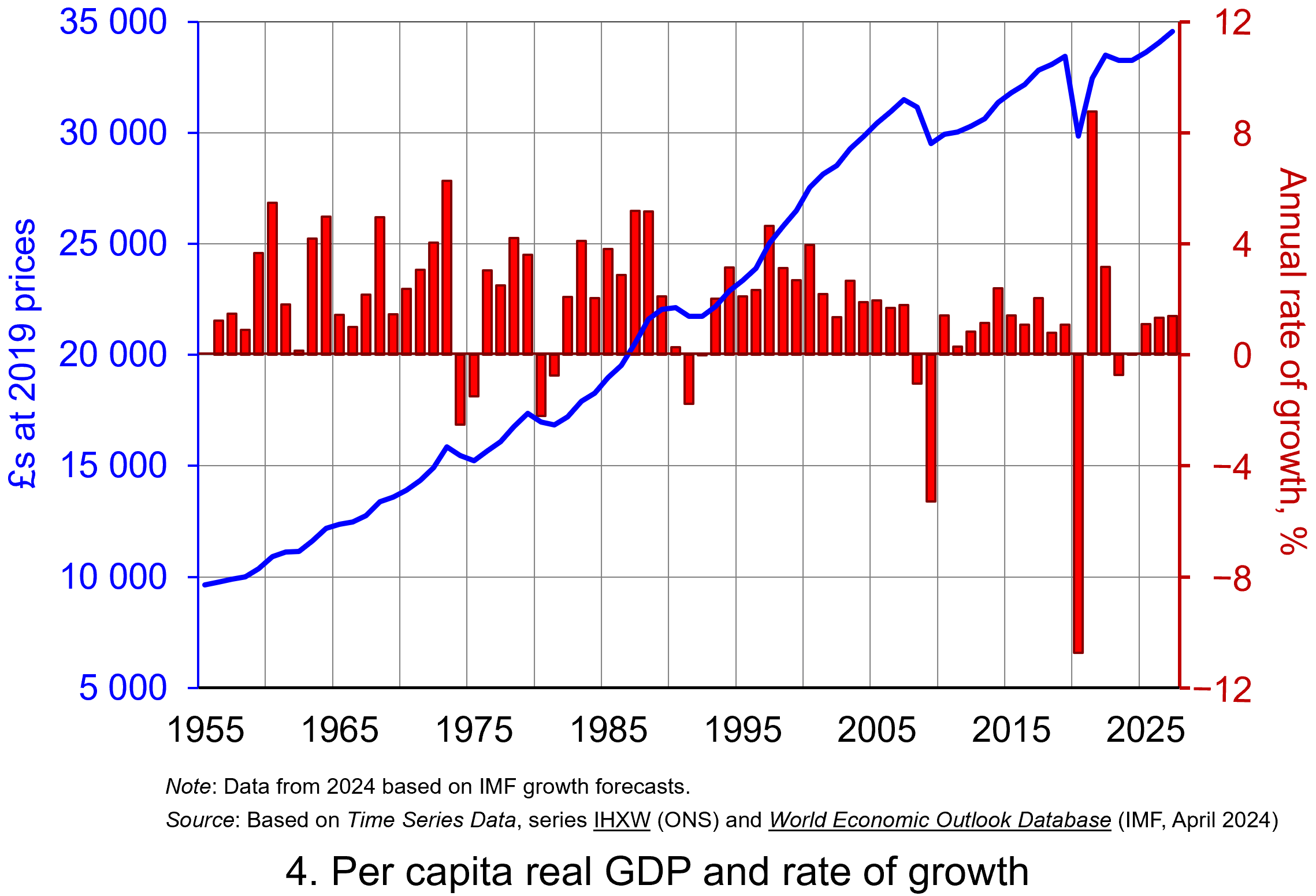 Our final chart therefore replicates Chart 3 but for real GDP per capita. Between 1955 and 2023 real GDP per capita grew by a factor of 3.45, which increases to 3.6 when we consider the period up to 2027. The average rate of growth of real GDP per capita up to 2023 was 1.87 per cent (lower than the 2.34 per cent increase in real GDP).
But the rate of increase in real GDP per capita was much higher before 2007 than it has been since. If we look at the period up to 2007 and, hence, before the global financial crisis, the figure is 2.32 per cent (2.7 per cent for real GDP), whereas from 2008 to 2023 the average rate of growth of real GDP per capita was a mere 0.42 per cent (1.1 per cent for real GDP). (Click here to download a PowerPoint copy of the chart.)
The final chart therefore reiterates the messages from recent blogs, such as Getting Real with Pay and The Productivity Puzzle, that long-term economic growth and the growth of real wages have slowed dramatically since the financial crisis. This has had important implications for the wellbeing of all sectors of the economy. The stagnation of living standards is therefore one of the most important economic issues of our time. It is one that the incoming Labour government will be keen to address.
Data and Reports
Articles
Questions
- What do you understand by the term ‘macroeconomic environment’? What data could be used to describe the macroeconomic environment?
- When a country experiences positive rates of inflation, which is higher: nominal economic growth or real economic growth?
- Does an increase in nominal GDP mean a country’s production has increased? Explain your answer.
- Does a decrease in nominal GDP mean a country’s production has decreased? Explain your answer.
- Why does a change in the growth of real GDP allow us to focus on what has happened to the volume of production?
- What does the concept of the ‘business cycle’ have to do with real rates of economic growth?
- When would falls in real GDP be classified as a recession?
- Distinguish between the concepts of ‘short-term growth’ and ‘longer-term growth’.
- What do you understand by the term ‘persistence’ in macroeconomics? Given examples of persistence effects and the means by which they can be generated?
- Discuss the proposition that the pandemic could have a positive effect on longer-term growth rates because of the ways that people and business have had to adapt.
 The following blog is inspired by my teaching of macroeconomic issues to my final year students at Aston University. In the classes we’ve been discussing important aspects of monetary and fiscal policy design. What has become clear to me and my students is that the trade-offs which characterise the discipline of economics are certainly alive and well in the current environment in which monetary and fiscal policy choices are being made.
To demonstrate this we consider here some of the discussions we’ve had in class around central bank independence and monetary policy mandates. We’ve also looked at fiscal policy. Here we’ve examined the state of the public finances and the importance that seems to be attached to debt stabilisation and the imposition of debt rules.
Delegation and central bank mandates
My teaching this term began by introducing my students to one of the most important and influential monetary policy models. This is the model of Kydland and Prescott. Their model, published in the Journal of Political Economy in 1977 has become the theoretical bedrock for the modern-day operational independence of central banks.1
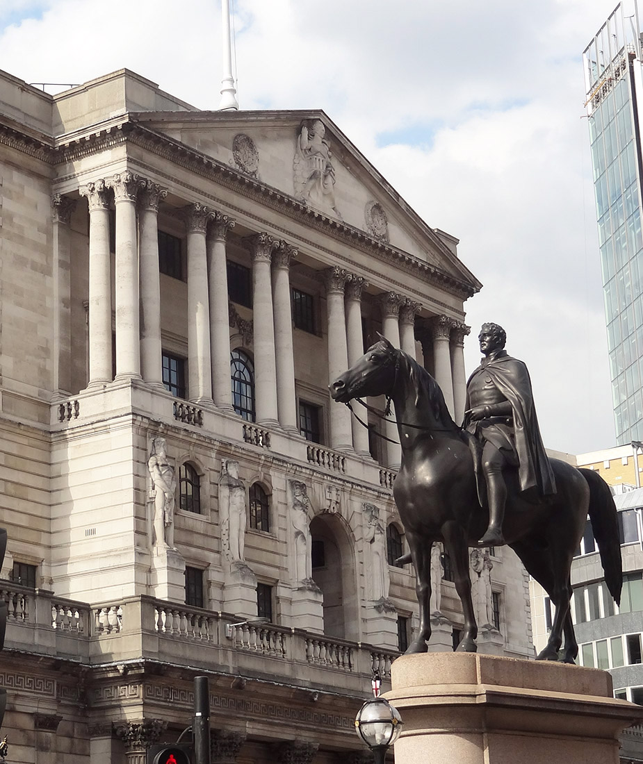 The model explores how systemically high inflation can become established in economies when policymakers have the political incentive to lower unemployment or increase output above its long-run equilibrium value. This may be the case if governments operate monetary policy rather than the central bank (of if the central bank operates monetary policy but follows government objectives). By adopting expansionary monetary policy, governments can increase their popularity.
But this is likely to be short-lived, as any increased economic activity will only be temporary (assuming that the natural-rate hypothesis holds). Soon, inflation will rise.
But, if an election is on the horizon, there may be enough time to boost output and employment before inflation rises. In other words, an expectations-augmented Phillips curve may present governments with an incentive to loosen monetary policy and worry about the inflation consequences after the election.
However, the resulting ‘inflation surprise’ through the loosening of monetary policy means a fall in real pay and therefore in purchasing power. If people suspect that governments will be tempted to loosen policy, they will keep their expectations of inflation higher than the socially optimal inflation rate. Consequently, low-inflation targets lack credibility when governments have the temptation to loosen monetary policy. Such targets are time-inconsistent because governments have an incentive to renege and deliver higher inflation through a looser monetary policy. The result is an inflation bias.
Central bank independence
To prevent this inflationary bias arising, many central banks around the world have been given some form of operational independence with a mandate centred around an inflation-rate target. By delegating monetary policy to a more conservative central bank, the problem of inflationary bias can be addressed.
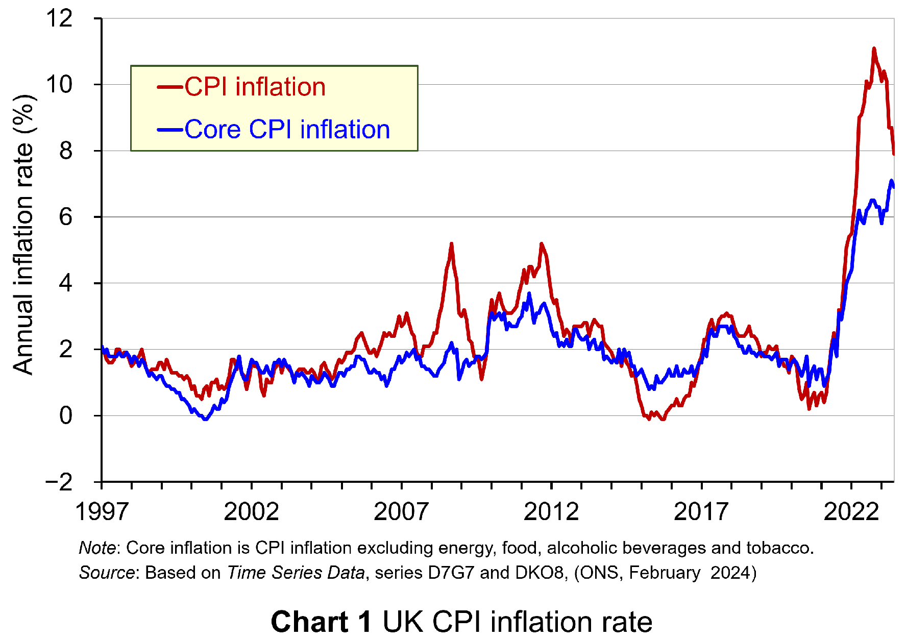 Yet central bank independence is not without its own issues and this has been an important part of the discussions with my students. Today, many economies are continuing to experience the effects of the inflationary shocks that began in 2021 (see Chart 1 for the UK CPI inflation rate: click here for a PowerPoint). The question is whether the appointment of a conservative or hard-nosed hawkish central banker trades off the stabilisation of inflation for greater volatility in output or unemployment.
The inflation–output stabilisation trade-off is closely associated with the works of Kenneth Rogoff2 and John Taylor3. The latter is known for his monetary policy rule, which has become known as the ‘Taylor rule’. This advocates that a rules-based central bank ought to place weight on both inflation and output stabilisation.
This is not without its own issues, however, since, by also placing weight on output stabilisation, we are again introducing the possibility of greater inflationary bias in policy making. Hence, while the act of delegation and a rules- or target-based approach may mitigate the extent of the bias relative to that in the Kydland and Prescott model, there nonetheless still remain issues around the design of the optimal framework for the conduct of monetary policy.
Indeed, the announcement that the UK had moved into recession in the last two quarters of 2023 can be seen as evidence that an otherwise abstract theoretical trade-off between inflation and output stabilisation is actually very real.
My classroom discussions have also shown how economic theory struggles to identify an optimal inflation-rate target. Beyond accepting that a low and stable inflation rate is desirable, it is difficult to address fully the student who asks what is so special about a 2% inflation target. Would not a 3% target, for example, be preferable, they might ask?
Whilst this may sound somewhat trivial, it has real-world consequences. In a world that now seems to be characterised by greater supply-side volatility and by more frequent inflation shocks than we were used to in recent history, might a higher inflation rate target be preferable? Certainly, one could argue that, with an inflation–output stabilisation trade-off, there is the possibility that monetary policy could be unduly restrictive in our potential new macroeconomic reality. Hence, we might come to see governments and central banks in the near future revisiting the mandates that frame the operation of their monetary policy. Time will tell.
Fiscal policy and debt stabilisation
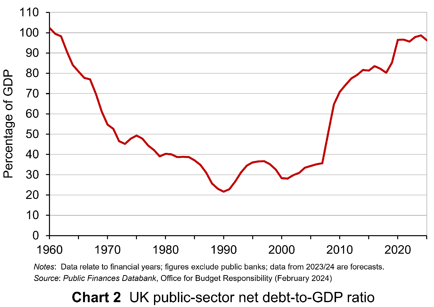 The second topic area that I have been discussing in my final-year macroeconomics classes has centred around fiscal policy and the state of the public finances. The context for this is that we have seen a significant increase in public debt-to-GDP ratios over the past couple of decades as the public sector has attempted to absorb significant economic shocks. These include the global financial crisis of 2007–8, the COVID-19 pandemic and the cost-of-living crisis. These interventions in the case of the UK have seen its public debt-to-GDP ratio more than triple since the early 2000s to close to 100% (see Chart 2: click here for a PowerPoint).
Understandably, given the stresses placed on the public finances, economists have increasingly debated issues around debt sustainability. These debates have been mirrored by politicians and policymakers. A key question is whether to have a public debt rule. The UK has in recent years adopted such a rule. The arguments for a rule centre on ensuring sound public finances and maintaining the confidence of investors to purchases public debt. A debt rule therefore places a discipline on fiscal policy, with implications for taxation and spending.
How easy it is to stick to a debt rule depends on three key factors. It will be harder to stick to the rule:
- The higher the current debt-to-GDP ratio and hence the more it needs to be reduced to meet the rule.
- The higher the rate of interest and hence the greater the cost of servicing the public debt.
- The lower the rate of economic growth and hence the less quickly will tax revenues rise.
With a given debt-to-GDP ratio, a given average interest rate payable on its debt, and a given rate of economic growth, we can determine the primary fiscal balance relative to GDP a government would need to meet for the debt-to-GDP ratio to remain stable. This is known as the ‘debt-stabilising primary balance’. The primary balance is the difference between a government’s receipts and its expenditures less the interest payments on its debt.
 This fiscal arithmetic is important in determining a government’s fiscal choices. It shows the implications for spending and taxation. These implications become ever more important and impactful on people, businesses, and society when the fiscal arithmetic becomes less favourable. This is a situation that appears to be increasingly the case for many countries, including the UK, as the rate of interest on public debt rises relative to a country’s rate of economic growth. As this happens, governments are increasingly required to run healthier primary balances. This of course implies a tightening of their fiscal stance.
Hence, the fiscal conversations with my students have focused on both the benefits and the costs of debt-stabilisation. In respect of the costs, a few issues have arisen.
First, as with the inflation-rate target, it is hard to identify an optimal public debt-to-GDP ratio number. While the fiscal arithmetic may offer some clue, it is not straightforward to address the question as to whether a debt-to-GDP ratio of say 100% or 120% would be excessive for the UK.
Second, it is possible that the debt stabilisation itself can make the fiscal arithmetic of debt stabilisation more difficult. This occurs if fiscal consolidation itself hinders long-term economic growth, which then makes the fiscal arithmetic more difficult. This again points to the difficulties in designing policy frameworks, whether they be for monetary or fiscal policy.
Third, a focus on debt stabilisation alone ignores the fact that there are two sides to any sector’s balance sheet. It would be very unusual when assessing the well-being of businesses or households if we were to ignore the asset side of their balance sheet. Yet, this is precisely the danger of focusing on public debt at the exclusion of what fiscal choices can mean for public-sector assets, from which we all can potentially benefit. Hence, some would suggest a more balanced approach to assessing the soundness of the public finances might involve a net worth (assets less liabilities) measure. This has parallels with the debates around whether mandates of central banks should be broader.
Applications in macroeconomics
What my teaching of a topics-based macroeconomics module this term has vividly demonstrated is that concepts, theories, and models come alive, and are capable of being understood better, when they are used to shine a light on real-world issues. The light being shone on monetary and fiscal policy in today’s turbulent macroeconomic environment is perhaps understandably very bright.
Indeed, the light being shone on fiscal policy in the UK and some other countries facing an upcoming election, is intensified further with the state of the public finances shaping much of the public discourse on fiscal choices. Hopefully, my students will continue to debate these important issues beyond their graduation, stressing their importance for people’s lives and, in doing so, going beyond the abstract.
References
- Rules rather than discretion: The inconsistency of optimal plans
The Journal of Political Economy, Finn E Kydland and Edward C. Prescott (1977, 85(3), pp 473–92)
- The optimal degree of commitment to an intermediate monetary target
Quarterly Journal of Economics, Kenneth Rogoff (November 1985, 100(4), pp 1169–89)
- Discretion versus policy rules in practice
Carnegie-Rochester Conference Series on Public Policy, John B Taylor (December 1993, 39, pp 195–214)
Articles
Questions
- What is meant by time-inconsistent monetary policy announcements? How has this concept been important for the way in which many central banks now conduct monetary policy?
- What is meant by a ‘conservative’ central banker? Why is the appointment of this type of central banker thought to be important in affecting inflation?
- What is the contemporary macroeconomic relevance of the inflation–output (or inflation–unemployment) stabilisation trade-off?
- How is the primary balance different from the actual budget balance?
- What do you understand by the concept of ‘the fiscal arithmetic’. Explain how each element of the fiscal arithmetic affects the debt-stabilising primary balance?
- Analyse the costs of benefits of a debt-based fiscal rule.
 It’s two years since Russia invaded Ukraine. Western countries responded by imposing large-scale sanctions. These targeted a range of businesses, banks and other financial institutions, payments systems and Russian exports and imports. Some $1 trillion of Russian assets were frozen. Many Western businesses withdrew from Russia or cut off commercial ties. In addition, oil and gas imports from Russia have been banned by most developed countries and some developing countries, and a price cap of $60 per barrel has been imposed on Russian oil. What is more, sanctions have been progressively tightened over the past two years. For example, on the second anniversary of the invasion, President Biden announced more than 500 new sanctions against individuals and companies involved in military production and supply chains and in financing Russia’s war effort.
The economy in Russia has also been affected by large-scale emigration of skilled workers, the diversion of workers to the armed forces and the diversion of capital and workers to the armaments industry.
So has the economy of Russia been badly affected by sanctions and these other factors? The IMF in its World Economic Forecast of April 2022 predicted that the Russian economy would experience a steep, two-year recession. But, the Russian economy has fared much better than first predicted and the steep recession never materialised.
In this blog we look at Russia’s economic performance. First, we examine why the Russian economy seems stronger today than forecast two years ago. Then we look at its economic weaknesses directly attributable to the war.
Apparent resilience of the Russian economy
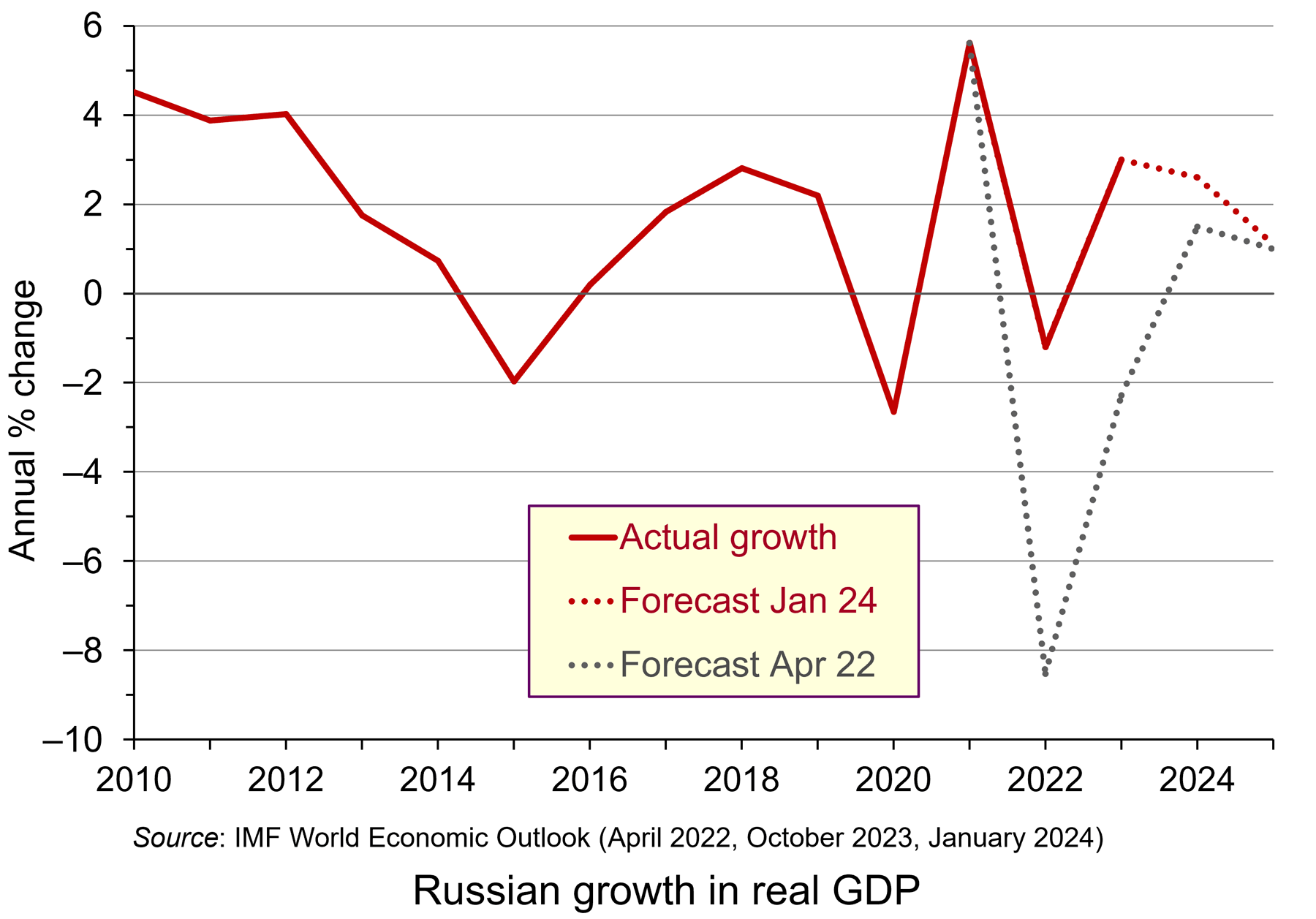 GDP forecasts have proved wrong. In April 2022, just after the start of the war, the IMF was forecasting that the Russian economy would decline by 8.5% in 2022 and by 2.3% in 2023 and grow by just 1.5% in 2024. In practice, the economy declined by only 1.2% in 2022 and grew by 3.0% in 2023. It is forecast by the IMF to grow by 2.6% in 2024. This is illustrated in the chart (click here for a PowerPoint).
Similarly, inflation forecasts have proved wrong. In April 2022, Russian consumer price inflation was forecast to be 21.3% in 2022 and 14.3% in 2023. In practice, inflation was 13.8% in 2022 and 7.4% in 2023. What is more, consumer spending in Russia has remained buoyant. In 2023, retail sales rose by 10.2% in nominal terms – a real rise of 2.8%. Wage growth has been strong and unemployment has remained low, falling from just over 4% in February 2022 to just under 3% today.
So why has the Russian economy seemingly weathered the war so successfully?
 The first reason is that, unlike Ukraine, very little of its infrastructure has been destroyed. Even though it has lost a lot of its military capital, including 1120 main battle tanks and some 2000 other armoured vehicles, virtually all of its production capacity remains intact. What is more, military production is replacing much of the destroyed vehicles and equipment.
The second is that its economy started the war in a strong position economically. In 2021, it had a surplus on the current account of its balance of payments of 6.7% of GDP, reflecting large revenues from oil, gas and mineral exports. This compares with a G7 average deficit of 0.7%. It had fiscal surplus (net general government lending) of 0.8% of GDP. The G7 countries had an average deficit of 9.1% of GDP. Its gross general government debt was 16% of GDP. The G7’s was an average of 134%. This put Russia in a position to finance the war and gave it a considerable buffer against economic sanctions.
 The third reason is that Russia has been effective in switching the destinations of exports and sources of imports. Trade with the West, Japan and South Korea has declined, but trade with China and various neutral countries, such as India have rapidly increased. Take the case of oil: in 2021, Russia exported 4.4 billion barrels of oil per day to the USA, the EU, the UK, Japan and South Korea. By 2023, this had fallen to just 0.6 billion barrels. By contrast, in 2021, it exported 1.9 billion barrels per day to China, India and Turkey. By 2023, this had risen to 4.9 billion. Although exports of natural gas have fallen by around 42% since 2021, Russian oil exports have remained much the same at around 7.4 million barrels per day (until a voluntary cut of 0.5 billion barrels per day in 2024 Q1 as part of an OPEC+ agreement to prop up the price of oil).
China is now a major supplier to Russia of components (some with military uses), commercial vehicles and consumer products (such as cars and electrical goods). Total trade with China (both imports and exports) was worth $147 billion in 2021. By 2023, this had risen to $240 billion.
The use of both the Chinese yuan and the Russian rouble (or ruble) has risen dramatically as a means of payment for Russian imports. Their share has risen from around 5% in 2021 (mainly roubles) to nearly 75% in 2023 (just over 37% in each currency). Switching trade and payment methods has helped Russia to circumvent many of the sanctions.
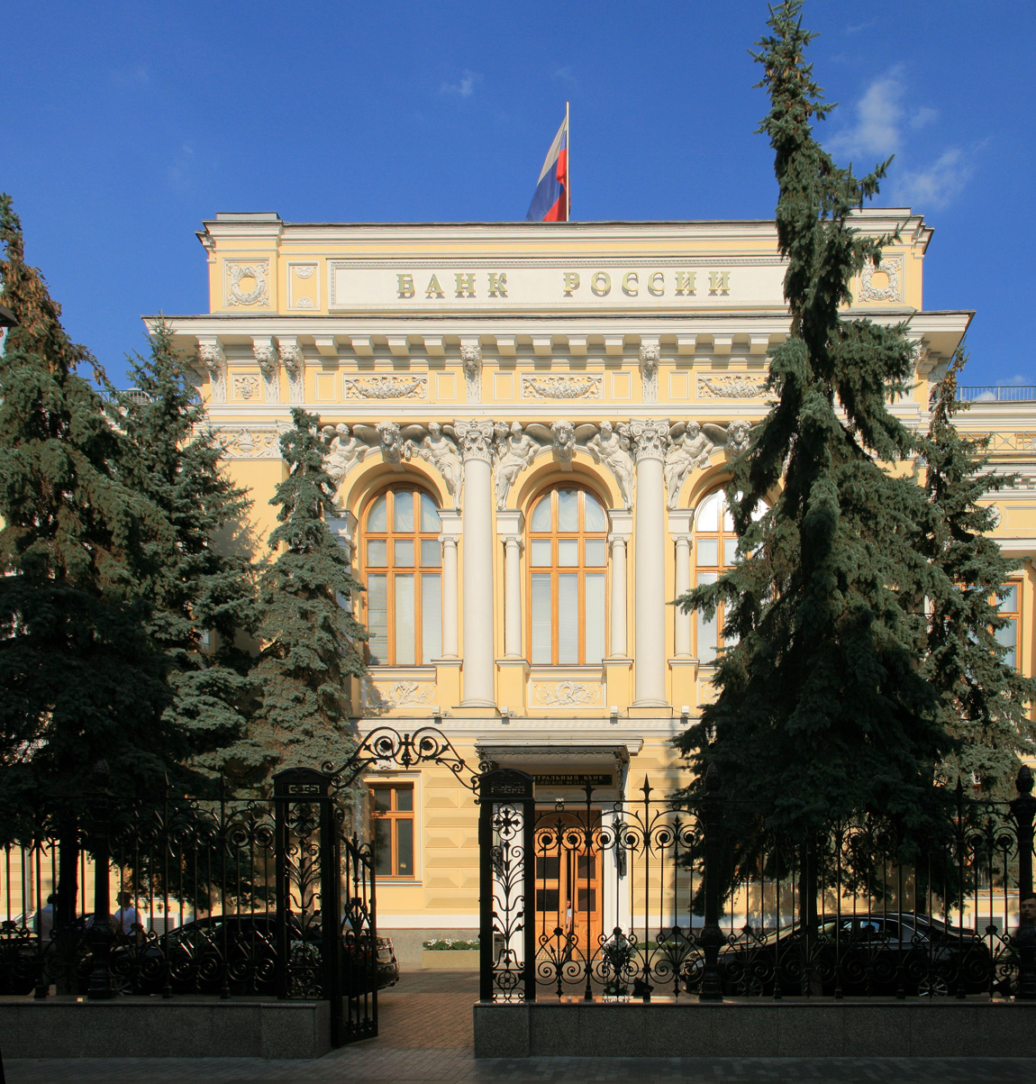 The fourth reason is that Russia has a strong and effective central bank. It has successfully used interest rates to control inflation, which is expected to fall from 7.4% in 2023 to under 5% this year and then to its target of 4% in subsequent years. The central bank policy rate was raised from 8.5% to 20% in February 2022. It then fell in steps to 7.5% in September 2022, where it remained until August 2023. It was then raised in steps to peak at 16% in December 2023, where it remains. There is a high level of confidence that the Russian central bank will succeed in bringing inflation back to target.
The fifth reason is that the war has provided a Keynesian stimulus to the economy. Military expenditure has doubled as a share of GDP – from 3.7% of GDP in 2021 to 7.5% in 2024. It now accounts for around 40% of government expenditure. The boost that this has given to production and employment has helped achieve the 3% growth rate in 2023, despite the dampening effect of a tight monetary policy.
Longer-term weaknesses
Despite the apparent resilience of the economy, there are serious weaknesses that are likely to have serious long-term effects.
There has been a huge decline in the labour supply as many skilled and professional workers have move abroad to escape the draft and as many people have been killed in battle. The shortage of workers has led to a rise in wages. This has been accompanied by a decline in labour productivity, which is estimated to have been around 3.6% in 2023.
 Higher wages and lower productivity is putting a squeeze on firms’ profits. This is being exacerbated by higher taxes on firms to help fund the war. Lower profit reduces investment and is likely to have further detrimental effects on labour productivity.
Although Russia has managed to circumvent many of the sanctions, they have still had a significant effect on the supply of goods and components from the West. As sanctions are tightened further, so this is likely to have a direct effect on production and living standards. Although GDP is growing, non-military production is declining.
The public finances at the start of the war, as we saw above, were strong. But the war effort has turned a budget surplus of 0.8% of GDP in 2021 to a deficit of 3.7% in 2023 – a deficit that will be difficult to fund with limited access to foreign finance and with domestic interest rates at 16%. As public expenditure on the military has increased, civilian expenditure has decreased. Benefits and expenditure on infrastructure are being squeezed. For example, public utilities and apartment blocks are deteriorating badly. This has a direct on living standards.
In terms of exports, although by diverting oil exports to China, India and other neutral countries Russia has manage to maintain the volume of its oil exports, revenue from them is declining. Oil prices have fallen from a peak of $125 per barrel in June 2022 to around $80 today. Production from the Arabian Gulf is likely to increase over the coming months, which will further depress oil prices.
Conclusions
With the war sustaining the Russian economy, it would be a problem for Russia if the war ended. If Russia won by taking more territory in Ukraine and forcing Ukraine to accept Russia’s terms for peace, the cost to Russia of rebuilding the occupied territories would be huge. If Russia lost territory and negotiated a settlement on Ukraine’s terms, the political cost would be huge, with a disillusioned Russian people facing reduced living standards that could lead to the overthrow of Putin. As The Conversation article linked below states:
A protracted stalemate might be the only solution for Russia to avoid total economic collapse. Having transformed the little industry it had to focus on the war effort, and with a labour shortage problem worsened by hundreds of thousands of war casualties and a massive brain drain, the country would struggle to find a new direction.
Articles
- How Russia’s economy survived two years of war
The Bell (23/2/24)
- How Russia uses China to get round sanctions
The Bell, Denis Kasyanchuk (20/2/24)
- As Ukraine’s economy burns, Russia clings to a semblance of prosperity
The Observer, Larry Elliott and Phillip Inman (24/2/24)
- ‘A lot higher than we expected’: Russian arms production worries Europe’s war planners
The Guardian, Andrew Roth (15/2/24)
- There are lessons from Russia’s GDP growth — but not the ones Putin thinks
Financial Times, Martin Sandbu (11/2/24)
 Russia’s economy going strong
DW, Miltiades Schmidt (21/2/24)
- The West tried to crush Russia’s economy. Why hasn’t it worked?
Politico, Nahal Toosi, Ari Hawkins, Koen Verhelst, Gabriel Gavin and Kyle Duggan (24/2/24)
- Don’t Buy Putin’s Bluff. The West Can Outspend Him.
Bloomberg UK, Editorial (23/2/24)
- Russia’s war economy cannot last but has bought time
BBC News, Faisal Islam (11/2/24)
- US targets Russia with more than 500 new sanctions
BBC News, George Wright and Will Vernon (24/2/24)
- Russia’s economy is now completely driven by the war in Ukraine – it cannot afford to lose, but nor can it afford to win
The Conversation, Renaud Foucart (22/2/24)
Questions
- Argue the case for and against including military production in GDP.
- How successful has the freezing of Russian assets been?
- How could Western sanctions against Russia be made more effective?
- What are the dangers to Western economies of further tightening financial sanctions against Russia?
- Would it be a desirable policy for a Western economy to divert large amounts of resources to building public infrastructure?
- Has the Ukraine war hastened the rise of the Chinese yuan as a reserve currency?
- How would you summarise Russia’s current public finances?
- How would you set about estimating the cost to Russia of its war with Ukraine?
 Artificial intelligence is having a profound effect on economies and society. From production, to services, to healthcare, to pharmaceuticals; to education, to research, to data analysis; to software, to search engines; to planning, to communication, to legal services, to social media – to our everyday lives, AI is transforming the way humans interact. And that transformation is likely to accelerate. But what will be the effects on GDP, on consumption, on jobs, on the distribution of income, and human welfare in general? These are profound questions and ones that economists and other social scientists are pondering. Here we look at some of the issues and possible scenarios.
According to the Merrill/Bank of America article linked below, when asked about the potential for AI, ChatGPT replied:
AI holds immense potential to drive innovation, improve decision-making processes and tackle complex problems across various fields, positively impacting society.
But the magnitude and distribution of the effects on society and economic activity are hard to predict. Perhaps the easiest is the effect on GDP. AI can analyse and interpret data to meet economic goals. It can do this much more extensively and much quicker than using pre-AI software. This will enable higher productivity across a range of manufacturing and service industries. According to the Merrill/Bank of America article, ‘global revenue associated with AI software, hardware, service and sales will likely grow at 19% per year’. With productivity languishing in many countries as they struggle to recover from the pandemic, high inflation and high debt, this massive boost to productivity will be welcome.
But whilst AI may lead to productivity growth, its magnitude is very hard to predict. Both the ‘low-productivity future’ and the ‘high-productivity future’ described in the IMF article linked below are plausible. Productivity growth from AI may be confined to a few sectors, with many workers displaced into jobs where they are less productive. Or, the growth in productivity may affect many sectors, with ‘AI applied to a substantial share of the tasks done by most workers’.
Growing inequality?
 Even if AI does massively boost the growth in world GDP, the distribution is likely to be highly uneven, both between countries and within countries. This could widen the gap between rich and poor and create a range of social tensions.
In terms of countries, the main beneficiaries will be developed countries in North America, Europe and Asia and rapidly developing countries, largely in Asia, such as China and India. Poorer developing countries’ access to the fruits of AI will be more limited and they could lose competitive advantage in a number of labour-intensive industries.
Then there is growing inequality between the companies controlling AI systems and other economic actors. Just as companies such as Microsoft, Apple, Google and Meta grew rich as computing, the Internet and social media grew and developed, so these and other companies at the forefront of AI development and supply will grow rich, along with their senior executives. The question then is how much will other companies and individuals benefit. Partly, it will depend on how much production can be adapted and developed in light of the possibilities that AI presents. Partly, it will depend on competition within the AI software market. There is, and will continue to be, a rush to develop and patent software so as to deliver and maintain monopoly profits. It is likely that only a few companies will emerge dominant – a natural oligopoly.
Then there is the likely growth of inequality between individuals. The reason is that AI will have different effects in different parts of the labour market.
The labour market
 In some industries, AI will enhance labour productivity. It will be a tool that will be used by workers to improve the service they offer or the items they produce. In other cases, it will replace labour. It will not simply be a tool used by labour, but will do the job itself. Workers will be displaced and structural unemployment is likely to rise. The quicker the displacement process, the more will such unemployment rise. People may be forced to take more menial jobs in the service sector. This, in turn, will drive down the wages in such jobs and employers may find it more convenient to use gig workers than employ workers on full- or part-time contracts with holidays and other rights and benefits.
But the development of AI may also lead to the creation of other high-productivity jobs. As the Goldman Sachs article linked below states:
Jobs displaced by automation have historically been offset by the creation of new jobs, and the emergence of new occupations following technological innovations accounts for the vast majority of long-run employment growth… For example, information-technology innovations introduced new occupations such as webpage designers, software developers and digital marketing professionals. There were also follow-on effects of that job creation, as the boost to aggregate income indirectly drove demand for service sector workers in industries like healthcare, education and food services.
Nevertheless, people could still lose their jobs before being re-employed elsewhere.
The possible rise in structural unemployment raises the question of retraining provision and its funding and whether workers would be required to undertake such retraining. It also raises the question of whether there should be a universal basic income so that the additional income from AI can be spread more widely. This income would be paid in addition to any wages that people earn. But a universal basic income would require finance. How could AI be taxed? What would be the effects on incentives and investment in the AI industry? The Guardian article, linked below, explores some of these issues.
The increased GDP from AI will lead to higher levels of consumption. The resulting increase in demand for labour will go some way to offsetting the effects of workers being displaced by AI. There may be new employment opportunities in the service sector in areas such as sport and recreation, where there is an emphasis on human interaction and where, therefore, humans have an advantage over AI.
Another issue raised is whether people need to work so many hours. Is there an argument for a four-day or even three-day week? We explored these issues in a recent blog in the context of low productivity growth. The arguments become more compelling when productivity growth is high.
Other issues
AI users are not all benign. As we are beginning to see, AI opens the possibility for sophisticated crime, including cyberattacks, fraud and extortion as the technology makes the acquisition and misuse of data, and the development of malware and phishing much easier.
 Another set of issues arises in education. What knowledge should students be expected to acquire? Should the focus of education continue to shift towards analytical skills and understanding away from the simple acquisition of knowledge and techniques. This has been a development in recent years and could accelerate. Then there is the question of assessment. Generative AI creates a range of possibilities for plagiarism and other forms of cheating. How should modes of assessment change to reflect this problem? Should there be a greater shift towards exams or towards project work that encourages the use of AI?
Finally, there is the issue of the sort of society we want to achieve. Work is not just about producing goods and services for us as consumers – work is an important part of life. To the extent that AI can enhance working life and take away a lot of routine and boring tasks, then society gains. To the extent, however, that it replaces work that involved judgement and human interaction, then society might lose. More might be produced, but we might be less fulfilled.
Articles
- The Macroeconomics of Artificial Intelligence
IMF publications, Erik Brynjolfsson and Gabriel Unger (December 2023)
- Economic impacts of artificial intelligence (AI)
European Parliamentary Research Service, Marcin Szczepański (July 2019)
- Artificial intelligence: A real game changer
Chief Investment Office, Merrill/Bank of America (July 2023)
 Generative AI could raise global GDP by 7%
Goldman Sachs, Joseph Briggs (5/4/23)
- The macroeconomic impact of artificial intelligence
PwC, Jonathan Gillham, Lucy Rimmington, Hugh Dance, Gerard Verweij, Anand Rao, Kate Barnard Roberts and Mark Paich (February 2018)
- How genAI is revolutionizing the field of economics
CNN, Bryan Mena and Samantha Delouya (12/10/23)
- AI-powered digital colleagues are here. Some ‘safe’ jobs could be vulnerable.
BBC Worklife, Sam Becker (30/11/23)
- Generative AI and Its Economic Impact: What You Need to Know
Investopedia, Jim Probasco (1/12/23)
- AI is coming for our jobs! Could universal basic income be the solution?
The Guardian Philippa Kelly (16/11/23)
- CFPB chief’s warning: AI is a ‘natural oligopoly’ in the making
Politico, Sam Sutton (21/11/23)
Questions
- Which industries are most likely to benefit from the development of AI?
- Distinguish between labour-replacing and labour-augmenting technological progress in the context of AI.
- How could AI reduce the amount of labour per unit of output and yet result in an increase in employment?
- What people are most likely to (a) gain, (b) lose from the increasing use of AI?
- Is the distribution of income likely to become more equal or less equal with the development and adoption of AI? Explain.
- What policies could governments adopt to spread the gains from AI more equally?
 To finance budget deficits, governments have to borrow. They can borrow short-term by issuing Treasury bills, typically for 1, 3 or 6 months. These do not earn interest and hence are sold at a discount below the face value. The rate of discount depends on supply and demand and will reflect short-term market rates of interest. Alternatively, governments can borrow long-term by issuing bonds. In the UK, these government securities are known as ‘gilts’ or ‘gilt-edged securities’. In the USA they are known as ‘treasury bonds’, ‘T-bonds’ or simply ‘treasuries’. In the EU, countries separately issue bonds but the European Commission also issues bonds.
In the UK, gilts are issued by the Debt Management Office on behalf of the Treasury. Although there are index-linked gilts, the largest proportion of gilts are conventional gilts. These pay a fixed sum of money per annum per £100 of face value. This is known as the ‘coupon payment’ and the rate is set at the time of issue. The ‘coupon rate’ is the payment per annum as a percentage of the bond’s face value:

Payments are made six-monthly. Each issue also has a maturity date, at which point the bonds will be redeemed at face value. For example, a 4½% Treasury Gilt 2028 bond has a coupon rate of 4½% and thus pays £4.50 per annum (£2.25 every six months) for each £100 of face value. The issue will be redeemed in June 2028 at face value. The issue was made in June 2023 and thus represented a 5-year bond. Gilts are issued for varying lengths of time from 2 to 55 years. At present, there are 61 different conventional issues of bonds, with maturity dates varying from January 2024 to October 2073.
Bond prices
 Bonds can be sold on the secondary market (i.e. the stock market) before maturity. The market price, however, is unlikely to be the coupon price (i.e. the face value). The lower the coupon rate relative to current interest rates, the less valuable the bond will be. For example, if interest rates rise, and hence new bonds pay a higher coupon rate, the market price of existing bonds paying a lower coupon rate must fall. Thus bond prices vary inversely with interest rates.
The market price also depends on how close the bonds are to maturity. The closer the maturity date, the closer the market price of the bond will be to the face value.
Bond yields: current yield
A bond’s yield is the percentage return that a person buying the bond receives. If a newly issued bond is bought at the coupon price, its yield is the coupon rate.
However, if an existing bond is bought on the secondary market (the stock market), the yield must reflect the coupon payments relative to the purchase price, not the coupon price. We can distinguish between the ‘current yield’ and the ‘yield to maturity’.
The current yield is the coupon payment as a percentage of the current market price of the bond:

Assume a bond were originally issued at 2% (its coupon rate) and thus pays £2 per annum. In the meantime, however, assume that interest rates have risen and new bonds now have a coupon rate of 4%, paying £4 per annum for each £100 invested. To persuade people to buy old bonds with a coupon rate of 2%, their market prices must fall below their face value (their coupon price). If their price halved, then they would pay £2 for every £50 of their market price and hence their current yield would be 4% (£2/£50 × 100).
Bond yields: yield to maturity (YTM)
But the current yield does not give the true yield – it is only an approximation. The true yield must take into account not just the market price but also the maturity value and the length of time to maturity (and the frequency of payments too, which we will ignore here). The closer a bond is to its maturity date, the higher/lower will be the true yield if the price is below/above the coupon price: in other words, the closer will the market price be to the coupon price for any given market rate of interest.
A more accurate measure of a bond’s yield is thus the ‘yield to maturity’ (YTM). This is the interest rate which makes the present value of all a bond’s future cash flows equal to its current price. These cash flows include all coupon payments and the payment of the face value on maturity. But future cash flows must be discounted to take into account the fact that money received in the future is worth less than money received now, since money received now could then earn interest.
The yield to maturity is the internal rate of return (IRR) of the bond. This is the discount rate which makes the present value (PV) of all the bond’s future cash flows (including the maturity payment of the coupon price) equal to its current market price. For simplicity, we assume that coupon payments are made annually. The formula is the one where the bond’s current market price is given by:

Where: t is the year; n is the number of years to maturity; YTM is the yield to maturity.
Thus if a bond paid £5 each year and had a maturity value of £100 and if current interest rates were higher than 5%, giving a yield to maturity of 8%, then the bond price would be:

In other words, with a coupon rate of 5% and a higher YTM of 8%, the bond with a face value of £100 and five years to maturity would be worth only £88.02 today.
If you know the market price of a given bond, you can work out its YTM by substituting in the above formula. The following table gives examples.
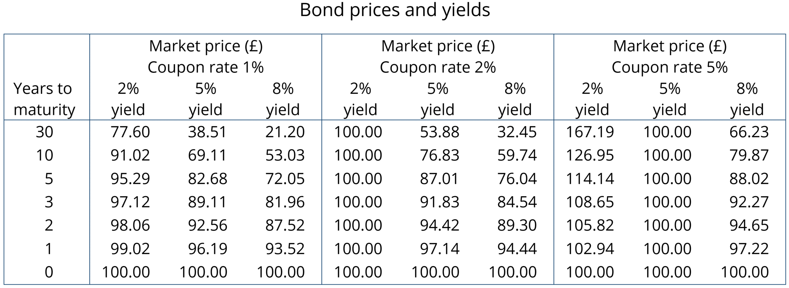
The higher the YTM, the lower the market price of a bond. Since the YTM reflects in part current rates of interest, so the higher the rate of interest, the lower the market price of any given bond. Thus bond yields vary directly with interest rates and bond prices vary inversely. You can see this clearly from the table. You can also see that market bond prices converge on the face value as the maturity date approaches.
Recent activity in bond markets
Investing in government bonds is regarded as very safe. Coupon payments are guaranteed, as is repayment of the face value on the maturity date. For this reason, many pension funds hold a lot of government bonds issued by financially trustworthy governments. But in recent months, bond prices in the secondary market have fallen substantially as interest rates have risen. For those holding existing bonds, this means that their value has fallen. For governments wishing to borrow by issuing new bonds, the cost has risen as they have to offer a higher coupon rate to attract buyers. This make it more expensive to finance government debt.
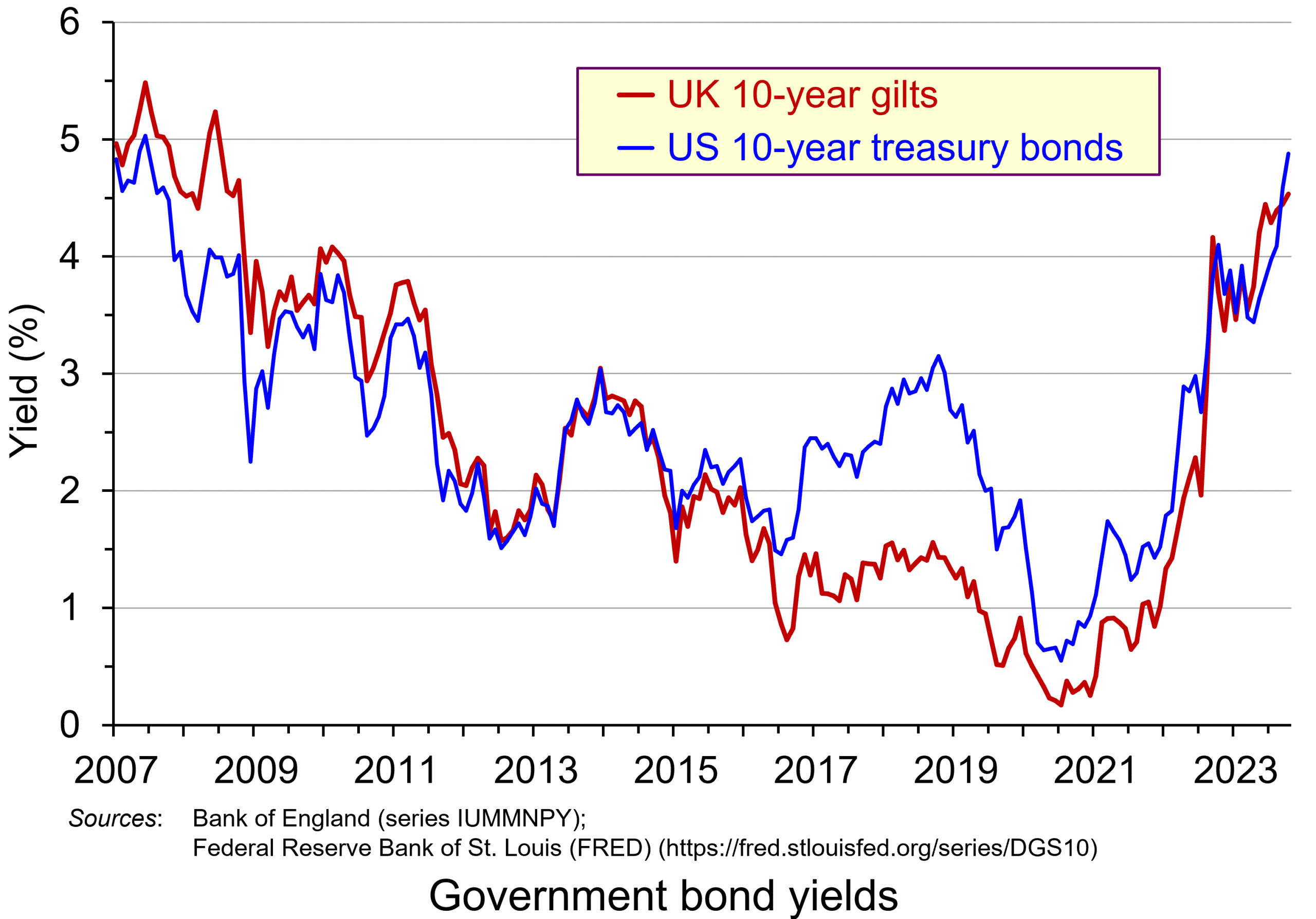 The chart shows the yield on 10-year government bonds. It is calculated using the ‘par value’ approach. This gives the coupon rate that would have to be paid for the market price of a bond to equal its face value. Clearly, as interest rates rise, a bond would have to pay a higher coupon rate for this to happen. (This, of course, is only hypothetical to give an estimate of market rates, as coupon rates are fixed at the time of a bond’s issue.)
Par values reflect both yield to maturity and also expectations of future interest rates. The higher people expect future interest rates to be, the higher must par values be to reflect this.
 In the years following the financial crisis of 2007–8 and the subsequent recession, and again during the COVID pandemic, central banks cut interest rates and supported this by quantitative easing. This involved central banks buying existing bonds on the secondary market and paying for them with newly created (electronic) money. This drove up bond prices and drove down yields (as the chart shows). This helped support the policy of low interest rates. This was a boon to governments, which were able to borrow cheaply.
This has all changed. With quantitative tightening replacing quantitative easing, central banks have been engaging in asset sales, thereby driving down bond prices and driving up yields. Again, this can be seen in the chart. This has helped to support a policy of higher interest rates.
Problems of higher bond yields/lower bond prices
Although lower bond prices and higher yields have supported a tighter monetary policy, which has been used to fight inflation, this has created problems.
First, it has increased the cost of financing government debt. In 2007/8, UK public-sector net debt was £567bn (35.6% of GDP). The Office for Budget Responsibility forecasts that it will be £2702bn (103.1% of GDP in the current financial year – 2023/24). Not only, therefore, are coupon rates higher for new government borrowing, but the level of borrowing is now a much higher proportion of GDP. In 2020/21, central government debt interest payments were 1.2% of GDP; by 2022/23, they were 4.4% (excluding interest on gilts held in the Bank of England, under the Asset Purchase Facility (quantitative easing)).
 In the USA, there have been similar increases in government debt and debt interest payments. Debt has increased from $9tn in 2007 to $33.6tn today. Again, with higher interest rates, debt interest as a percentage of GDP has risen: from 1.5% of GDP in 2021 to a forecast 2.5% in 2023 and 3% in 2024. What is more, 31 per cent of US government bonds will mature next year and will need refinancing – at higher coupon rates.
There is a similar picture in other developed countries. Clearly, higher interest payments leave less government revenue for other purposes, such as health and education.
Second, many pension funds, banks and other investment companies hold large quantities of bonds. As their price falls, so this reduces the value of these companies’ assets and makes it harder to finance new purchases, or payments or loans to customers. However, the fact that new bonds pay higher interest rates means that when existing bond holdings mature, the money can be reinvested at higher rates.
Third, bonds are often used by companies as collateral against which to borrow and invest in new capital. As bond prices fall, this can hamper companies’ ability to invest, which will lead to lower economic growth.
Fourth, higher bond yields divert demand away from equities (shares). With equity markets falling back or at best ceasing to rise, this erodes the value of savings in equities and may make it harder for firms to finance investment through new issues.
At the core of all these problems is inflation and budget deficits. Central banks have responded by raising interest rates. This drives up bond yields and drives down bond prices. But bond prices and yields depend not just on current interest rates, but also on expectations about future interest rates. Expectations currently are that budget deficits will be slow to fall as governments seek to support their economies post-COVID. Also expectations are that inflation, even though it is falling, is not falling as fast as originally expected – a problem that could be exacerbated if global tensions increase as a result of the ongoing war in Ukraine, the Israel/Gaza war and possible increased tensions with China concerning disputes in the China Sea and over Taiwan. Greater risks drive up bond yields as investors demand a higher interest premium.
Articles
Information and data
Questions
- Why do bond prices and bond yields vary inversely?
- How are bond yields and prices affected by expectations?
- Why are ‘current yield’ and ‘yield to maturity’ different?
- What is likely to happen to bond prices and yields in the coming months? Explain your reasoning.
- What constraints do bond markets place on fiscal policy?
- Would it be desirable for central banks to pause their policy of quantitative tightening?
 In the second of a series of blogs looking at applications of the distinction between nominal and real indicators, we revisit the blog Getting Real with Growth last updated in October 2021.
 Chart 1 shows current-price estimates of GDP from 1955, when the value of GDP was estimated at £19.2 billion. The £2.687 trillion figure recorded for 2023 is an increase of over 140 times that in 1955, a figure that rises to 160 times if we compare the 1950 value with the latest IMF estimate for 2027. However, if we want to make a more meaningful comparison of the country’s national income we need to adjust for inflation. (Click here to download a PowerPoint of the chart.)
 Between 1955 and 2023 real GDP increased 4.6 times. If we extend the period to 2027, again using the latest IMF estimates, the increase is 4.9 times. Because we have removed the effect of inflation, the real growth figure is much lower than the nominal growth figure.
 Chart 2 shows the annual rate of growth in real GDP each year from 1955 to 2025. From it, we see the inherent instability that is a key characteristic of the macroeconomic environment. This instability is, of course, mirrored in the output path of real GDP in Chart 1, but the annual rates of growth show the instability more clearly. We can readily see the impact on national output of the global financial crisis of 2007–8 and the global COVID pandemic.
 The twin characteristics of growth can be seen simultaneously by combining the output path (shown by the levels of real GDP) with the annual rates of growth. This is shown in Chart 3. The longer-term growth seen in the economy’s output path is generally argued to be driven by the quantity and quality of the economy’s resources, and their effectiveness when combined in production (i.e. their productivity). In other words, it is the supply side of the economy that determines the trajectory of the output path over the longer term. (Click here to download a PowerPoint copy of the chart.)
 Our final chart therefore replicates Chart 3 but for real GDP per capita. Between 1955 and 2023 real GDP per capita grew by a factor of 3.45, which increases to 3.6 when we consider the period up to 2027. The average rate of growth of real GDP per capita up to 2023 was 1.87 per cent (lower than the 2.34 per cent increase in real GDP).
  The following blog is inspired by my teaching of macroeconomic issues to my final year students at Aston University. In the classes we’ve been discussing important aspects of monetary and fiscal policy design. What has become clear to me and my students is that the trade-offs which characterise the discipline of economics are certainly alive and well in the current environment in which monetary and fiscal policy choices are being made.
 The model explores how systemically high inflation can become established in economies when policymakers have the political incentive to lower unemployment or increase output above its long-run equilibrium value. This may be the case if governments operate monetary policy rather than the central bank (of if the central bank operates monetary policy but follows government objectives). By adopting expansionary monetary policy, governments can increase their popularity.
 Yet central bank independence is not without its own issues and this has been an important part of the discussions with my students. Today, many economies are continuing to experience the effects of the inflationary shocks that began in 2021 (see Chart 1 for the UK CPI inflation rate: click
  The second topic area that I have been discussing in my final-year macroeconomics classes has centred around fiscal policy and the state of the public finances. The context for this is that we have seen a significant increase in public debt-to-GDP ratios over the past couple of decades as the public sector has attempted to absorb significant economic shocks. These include the global financial crisis of 2007–8, the COVID-19 pandemic and the cost-of-living crisis. These interventions in the case of the UK have seen its public debt-to-GDP ratio more than triple since the early 2000s to close to 100% (see Chart 2: click
  This fiscal arithmetic is important in determining a government’s fiscal choices. It shows the implications for spending and taxation. These implications become ever more important and impactful on people, businesses, and society when the fiscal arithmetic becomes less favourable. This is a situation that appears to be increasingly the case for many countries, including the UK, as the rate of interest on public debt rises relative to a country’s rate of economic growth. As this happens, governments are increasingly required to run healthier primary balances. This of course implies a tightening of their fiscal stance.
 It’s two years since Russia invaded Ukraine. Western countries responded by imposing
  GDP forecasts have proved wrong. In April 2022, just after the start of the war, the IMF was forecasting that the Russian economy would decline by 8.5% in 2022 and by 2.3% in 2023 and grow by just 1.5% in 2024. In practice, the economy declined by only 1.2% in 2022 and grew by 3.0% in 2023. It is forecast by the IMF to grow by 2.6% in 2024. This is illustrated in the chart (click
  The first reason is that, unlike Ukraine, very little of its infrastructure has been destroyed. Even though it has lost a lot of its military capital, including 1120 main battle tanks and some 2000 other armoured vehicles, virtually all of its production capacity remains intact. What is more, military production is replacing much of the destroyed vehicles and equipment.
 The third reason is that Russia has been effective in switching the destinations of exports and sources of imports. Trade with the West, Japan and South Korea has declined, but trade with China and various neutral countries, such as India have rapidly increased. Take the case of oil: in 2021, Russia exported 4.4 billion barrels of oil per day to the USA, the EU, the UK, Japan and South Korea. By 2023, this had fallen to just 0.6 billion barrels. By contrast, in 2021, it exported 1.9 billion barrels per day to China, India and Turkey. By 2023, this had risen to 4.9 billion. Although exports of natural gas have fallen by around 42% since 2021, Russian oil exports have remained much the same at around 7.4 million barrels per day (until a voluntary cut of 0.5 billion barrels per day in 2024 Q1 as part of an OPEC+ agreement to prop up the price of oil).
 The fourth reason is that Russia has a strong and effective central bank. It has successfully used interest rates to control inflation, which is expected to fall from 7.4% in 2023 to under 5% this year and then to its target of 4% in subsequent years. The central bank policy rate was raised from 8.5% to 20% in February 2022. It then fell in steps to 7.5% in September 2022, where it remained until August 2023. It was then raised in steps to peak at 16% in December 2023, where it remains. There is a high level of confidence that the Russian central bank will succeed in bringing inflation back to target.
 Higher wages and lower productivity is putting a squeeze on firms’ profits. This is being exacerbated by higher taxes on firms to help fund the war. Lower profit reduces investment and is likely to have further detrimental effects on labour productivity.
 Artificial intelligence is having a profound effect on economies and society. From production, to services, to healthcare, to pharmaceuticals; to education, to research, to data analysis; to software, to search engines; to planning, to communication, to legal services, to social media – to our everyday lives, AI is transforming the way humans interact. And that transformation is likely to accelerate. But what will be the effects on GDP, on consumption, on jobs, on the distribution of income, and human welfare in general? These are profound questions and ones that economists and other social scientists are pondering. Here we look at some of the issues and possible scenarios.
 Even if AI does massively boost the growth in world GDP, the distribution is likely to be highly uneven, both between countries and within countries. This could widen the gap between rich and poor and create a range of social tensions.
  In some industries, AI will enhance labour productivity. It will be a tool that will be used by workers to improve the service they offer or the items they produce. In other cases, it will replace labour. It will not simply be a tool used by labour, but will do the job itself. Workers will be displaced and structural unemployment is likely to rise. The quicker the displacement process, the more will such unemployment rise. People may be forced to take more menial jobs in the service sector. This, in turn, will drive down the wages in such jobs and employers may find it more convenient to use gig workers than employ workers on full- or part-time contracts with holidays and other rights and benefits.
 Another set of issues arises in education. What knowledge should students be expected to acquire? Should the focus of education continue to shift towards analytical skills and understanding away from the simple acquisition of knowledge and techniques. This has been a development in recent years and could accelerate. Then there is the question of assessment. Generative AI creates a range of possibilities for plagiarism and other forms of cheating. How should modes of assessment change to reflect this problem? Should there be a greater shift towards exams or towards project work that encourages the use of AI?
 To finance budget deficits, governments have to borrow. They can borrow short-term by
  Bonds can be sold on the secondary market (i.e. the stock market) before maturity. The market price, however, is unlikely to be the coupon price (i.e. the face value). The lower the coupon rate relative to current interest rates, the less valuable the bond will be. For example, if interest rates rise, and hence new bonds pay a higher coupon rate, the market price of existing bonds paying a lower coupon rate must fall. Thus bond prices vary inversely with interest rates.


 The chart shows the yield on 10-year government bonds. It is calculated using the ‘par value’ approach. This gives the coupon rate that would have to be paid for the market price of a bond to equal its face value. Clearly, as interest rates rise, a bond would have to pay a higher coupon rate for this to happen. (This, of course, is only hypothetical to give an estimate of market rates, as coupon rates are fixed at the time of a bond’s issue.)
  In the years following the financial crisis of 2007–8 and the subsequent recession, and again during the COVID pandemic, central banks cut interest rates and supported this by quantitative easing. This involved central banks buying existing bonds on the secondary market and paying for them with newly created (electronic) money. This drove up bond prices and drove down yields (as the chart shows). This helped support the policy of low interest rates. This was a boon to governments, which were able to borrow cheaply.
 In the USA, there have been similar increases in government debt and debt interest payments. Debt has increased from $9tn in 2007 to $33.6tn today. Again, with higher interest rates, debt interest as a percentage of GDP has risen: from 1.5% of GDP in 2021 to a forecast 2.5% in 2023 and 3% in 2024. What is more, 31 per cent of US government bonds will mature next year and will need refinancing – at higher coupon rates.