 In a blog in October 2024, we looked at global uncertainty and how it can be captured in a World Uncertainty Index. The blog stated that ‘We continue to live through incredibly turbulent times. In the past decade or so we have experienced a global financial crisis, a global health emergency, seen the UK’s departure from the European Union, and witnessed increasing levels of geopolitical tension and conflict’.
Since then, Donald Trump has been elected for a second term and has introduced sweeping tariffs. What is more, the tariffs announced on so-called ‘Liberation Day‘ have not remained fixed, but have fluctuated with negotiations and threatened retaliation. The resulting uncertainty makes it very hard for businesses to plan and many have been unwilling to commit to investment decisions. The uncertainty has been compounded by geopolitical events, such as the continuing war in Ukraine, the war in Gaza and the June 13 Israeli attack on Iran.
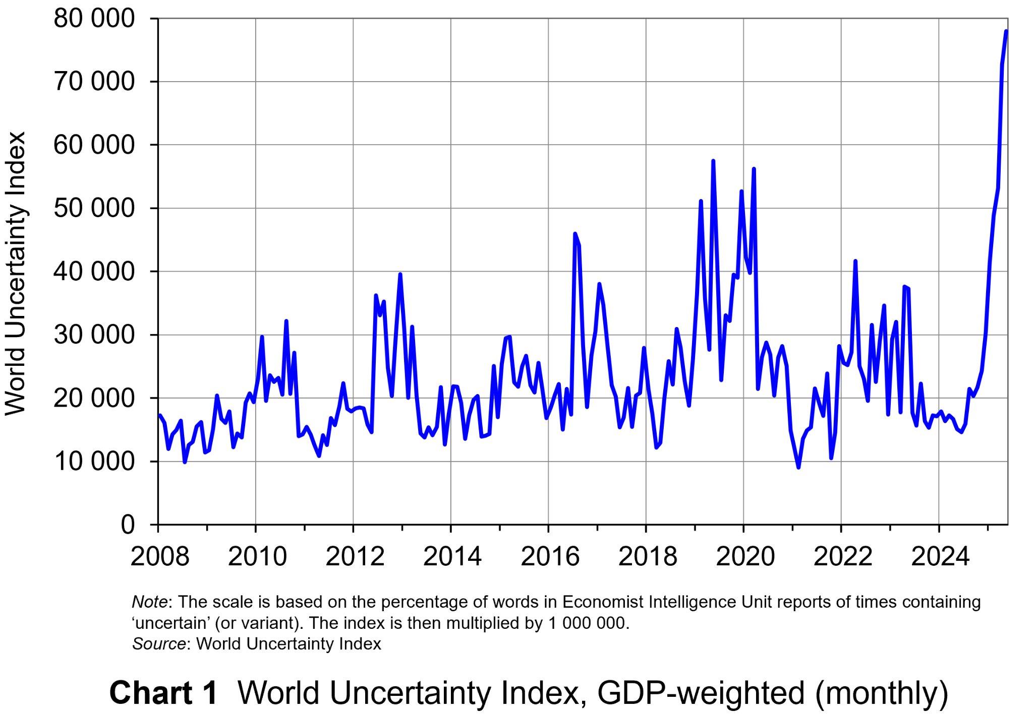 The World Uncertainty Index (WUI) tracks uncertainty around the world by applying a form of text mining known as ‘term frequency’ to the country reports produced by the Economist Intelligence Unit (EIU). The words searched for are ‘uncertain’, ‘uncertainty’ and ‘uncertainties’ and the number of times they occur as percentage of the total words is recorded. To produce the WUI this figure is then multiplied by 1m. A higher WUI number indicates a greater level of uncertainty.
The monthly global average WUI is shown in Chart 1 (click here for a PowerPoint). It is based on 71 countries. Since 2008 the WUI has averaged a little over 23 000: i.e. 2.3 per cent of the text in EIU reports contains the word ‘uncertainty’ or a close variant. In May 2025, it was almost 79 000 – the highest since the index was first complied in 2008. The previous highest was in March 2020, at the start of the COVID-19 outbreak, when the index rose to just over 56 000.
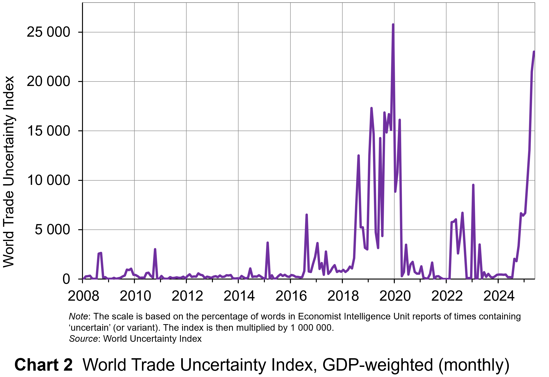 The second chart shows the World Trade Uncertainty Index (WTUI), published on the same site as the WUI (click here for a PowerPoint). The method adopted in its construction therefore mirrors that for the WUI but counts the number of times in EIU country reports ‘uncertainty’ is mentioned within proximity to a word related to trade, such as ‘protectionism’, ‘NAFTA’, ‘tariff’, ‘trade’, ‘UNCTAD’ or ‘WTO.’
The chart shows that in May 2025, the WTUI had risen to just over 23 000 – the second highest since December 2019, when President Trump imposed a new round of tariffs on Chinese imports and announced that he would restore steel tariffs on Brazil and Argentina. Since 2008, the WTUI has averaged just 2228.
It remains to be seen whether more stability in trade relations and geopolitics will allow WUI and WUTI to decline once more, or whether greater instability will simply lead to greater uncertainty, with damaging consequences for investment and also for consumption and employment.
Articles
Uncertainty Indices
Questions
- Explain what is meant by ‘text mining’. What are its strengths and weaknesses in assessing business, consumer and trade uncertainty?
- Explain how the UK Monthly EPU Index is derived.
- Why has uncertainty increased so dramatically since the start of 2025?
- Compare indices based on text mining with confidence indices.
- Plot consumer and business/industry confidence indicators for the past 24 months, using EC data. Do they correspond with the WUI?
- How may uncertainty affect consumers’ decisions?
 In a blog from March 2023 (reproduced below), we saw how there has been growing pressure around the world for employers to move to a four-day week. Increasing numbers of companies have adopted the model of 80% of the hours for 100% of the pay.
As we see below, the model adopted has varied across companies, depending on what was seen as most suitable for them. Some give everyone Friday off; others let staff choose which day to have off; others let staff work 80% of the hours on a flexible basis. Firms adopting the model have generally found that productivity and revenue have increased, as has employee well-being. To date, over 200 employers in the UK, employing more than 5000 people, have adopted a permanent four-day week.
This concept of 100-80-100, namely 100% of pay for 80% of hours, but 100% of output, has been trialled in several countries. In Germany, after trials over 2024, 73% of the companies involved plan to continue with the new model, with the remaining 27% either making minor tweaks or yet to decide. Generally hourly productivity rose, and in many cases total output also rose. As the fourth article below states:
The primary causal factor for this intriguing revelation was simple – efficiency became the priority. Reports from the trial showed that the frequency and duration of meetings was reduced by 60%, which makes sense to anyone who works in an office – many meetings could have been a simple email. 25% of companies tested introduced new digitised ways of managing their workflow to optimise efficiency.
Original post
In two previous posts, one at the end of 2019 and one in July 2021, we looked at moves around the world to introduce a four-day working week, with no increase in hours on the days worked and no reduction in weekly pay. Firms would gain if increased worker energy and motivation resulted in a gain in output. They would also gain if fewer hours resulted in lower costs.
Workers would be likely to gain from less stress and burnout and a better work–life balance. What is more, firms’ and workers’ carbon footprint could be reduced as less time was spent at work and in commuting.
If the same output could be produced with fewer hours worked, this would represent an increase in labour productivity measured in output per hour.
The UK’s poor productivity record since 2008
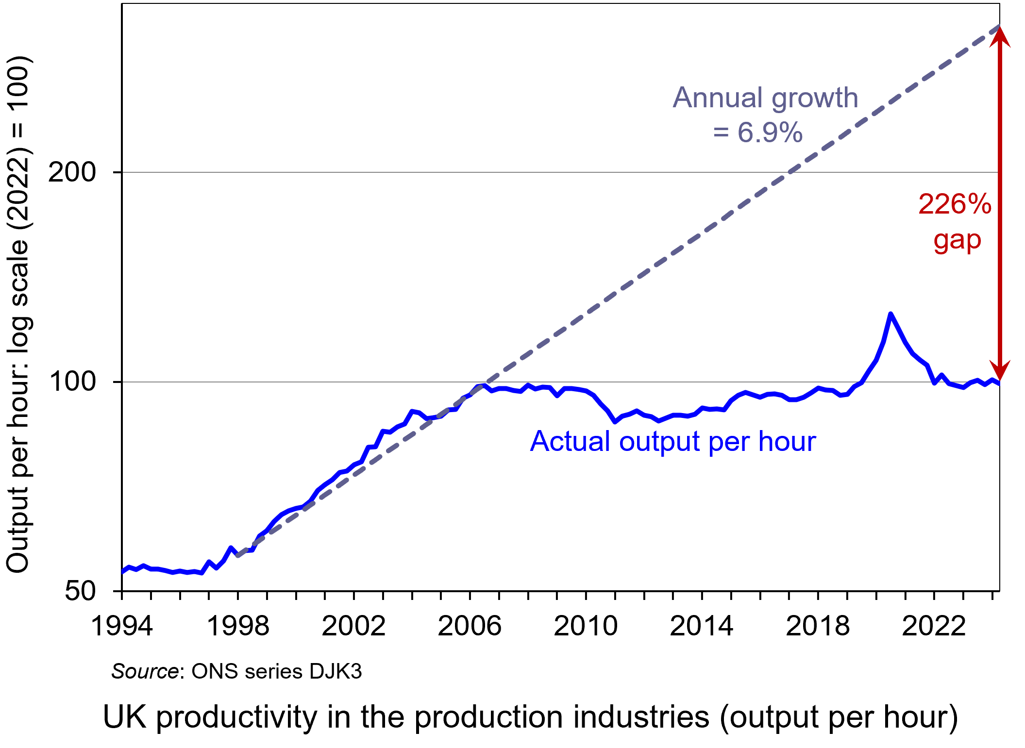 Since the financial crisis of 2007–8, the growth in UK productivity has been sluggish. This is illustrated in the chart, which looks at the production industries: i.e. it excludes services, where average productivity growth tends to be slower. The chart has been updated to 2024 Q2 – the latest data available. (Click here for a PowerPoint of the chart.)
Prior to the crisis, from 1998 to 2006, UK productivity in the production industries grew at an annual rate of 6.9%. From 2007 to the start of the pandemic in 2020, the average annual productivity growth rate in these industries was a mere 0.2%.
It grew rapidly for a short time at the start of the pandemic, but this was because many businesses temporarily shut down or went to part-time working, and many of these temporary job cuts were low-wage/low productivity jobs. If you take services, the effect was even stronger as sectors such as hospitality, leisure and retail were particularly affected and labour productivity in these sectors tends to be low. As industries opened up and took on more workers, so average productivity rapidly fell back. Since then productivity has flatlined.
If you project the average productivity growth rate from 1998 to 2007 of 6.9% forwards (see grey dashed line), then by 2024 Q3, output per hour in the production industries would have been 3.26 times higher than it actually was: a gap of 226%. This is a huge productivity gap.
 Productivity in the UK is lower than in many other competitor countries. According to the ONS, output per hour in the UK in 2021 was $59.14 in the UK. This compares with an average of $64.93 for the G7 countries, $66.75 in France, £68.30 in Germany, $74.84 in the USA, $84.46 in Norway and $128.21 in Ireland. It is lower, however, in Italy ($54.59), Canada ($53.97) and Japan ($47.28).
As we saw in the blog, The UK’s poor productivity record, low UK productivity is caused by a number of factors, not least the lack of investment in physical capital, both by private companies and in public infrastructure, and the lack of investment in training. Other factors include short-termist attitudes of both politicians and management and generally poor management practices. But one cause is the poor motivation of many workers and the feeling of being overworked. One solution to this is the four-day week.
Latest evidence on the four-day week
Results have just been released of a pilot programme involving 61 companies and non-profit organisations in the UK and nearly 3000 workers. They took part in a six-month trial of a four-day week, with no increase in hours on the days worked and no loss in pay for employees – in other words, 100% of the pay for 80% of the time. The trial was a success, with 91% of organisations planning to continue with the four-day week and a further 4% leaning towards doing so.
 The model adopted varied across companies, depending on what was seen as most suitable for them. Some gave everyone Friday off; others let staff choose which day to have off; others let staff work 80% of the hours on a flexible basis.
There was little difference in outcomes across different types of businesses. Compared with the same period last year, revenues rose by an average of 35%; sick days fell by two-thirds and 57% fewer staff left the firms. There were significant increases in well-being, with 39% saying they were less stressed, 40% that they were sleeping better; 75% that they had reduced levels of burnout and 54% that it was easier to achieve a good work–life balance. There were also positive environmental outcomes, with average commuting time falling by half an hour per week.
There is growing pressure around the world for employers to move to a four-day week and this pilot provides evidence that it significantly increases productivity and well-being.
Additional articles
Original set of articles
- Results from world’s largest 4 day week trial bring good news for the future of work
4 Day Week Global, Charlotte Lockhart (21/2/23)
- Four-day week: ‘major breakthrough’ as most UK firms in trial extend changes
The Guardian, Heather Stewart (21/2/23)
- Senedd committee backs four-day working week trial in Wales
The Guardian, Steven Morris (24/1/23)
- ‘Major breakthrough’: Most firms say they’ll stick with a four-day working week after successful trial
Sky News, Alice Porter (21/2/23)
- Major four-day week trial shows most companies see massive staff mental health benefits and profit increase
Independent, Anna Wise (21/2/23)
- Four-day week: Which countries have embraced it and how’s it going so far?
euronews, Josephine Joly and Luke Hurst (23/2/23)
- Firms stick to four-day week after trial ends
BBC News, Simon Read, Lucy Hooker & Emma Simpson (21/2/23)
- The climate benefits of a four-day workweek
BBC Future Planet, Giada Ferraglioni and Sergio Colombo (21/2/23)
- Four-day working week: why UK businesses and workers will continue with new work pattern, plus pros and cons
National World, Rochelle Barrand (22/2/23)
- Most companies in UK four-day week trial to continue with flexible working
Financial Times, Daniel Thomas and Emma Jacobs (21/2/23)
- The pros and cons of a four-day working week
Financial Times, Editorial (13/2/23)
- Explaining the UK’s productivity slowdown: Views of leading economists
VoxEU, Ethan Ilzetzki (11/3/20)
- Why the promised fourth industrial revolution hasn’t happened yet
The Conversation, Richard Markoff and Ralf Seifert (27/2/23)
Questions
- What are the possible advantages of moving to a four-day week?
- What are the possible disadvantages of moving to a four-day week?
- What types of companies or organisations are (a) most likely, (b) least likely to gain from a four-day week?
- Why has the UK’s productivity growth been lower than that of many of its major competitors?
- Why, if you use a log scale on the vertical axis, is a constant rate of growth shown as a straight line? What would a constant rate of growth line look like if you used a normal arithmetical scale for the vertical axis?
- Find out what is meant by the ‘fourth industrial revolution’. Does this hold out the hope of significant productivity improvements in the near future? (See, for example, last link above.)
 During the pandemic, most people who were not furloughed were forced to work from home. After lockdown restrictions were lifted, many employers decided to continue with people working remotely, at least for some of the time.
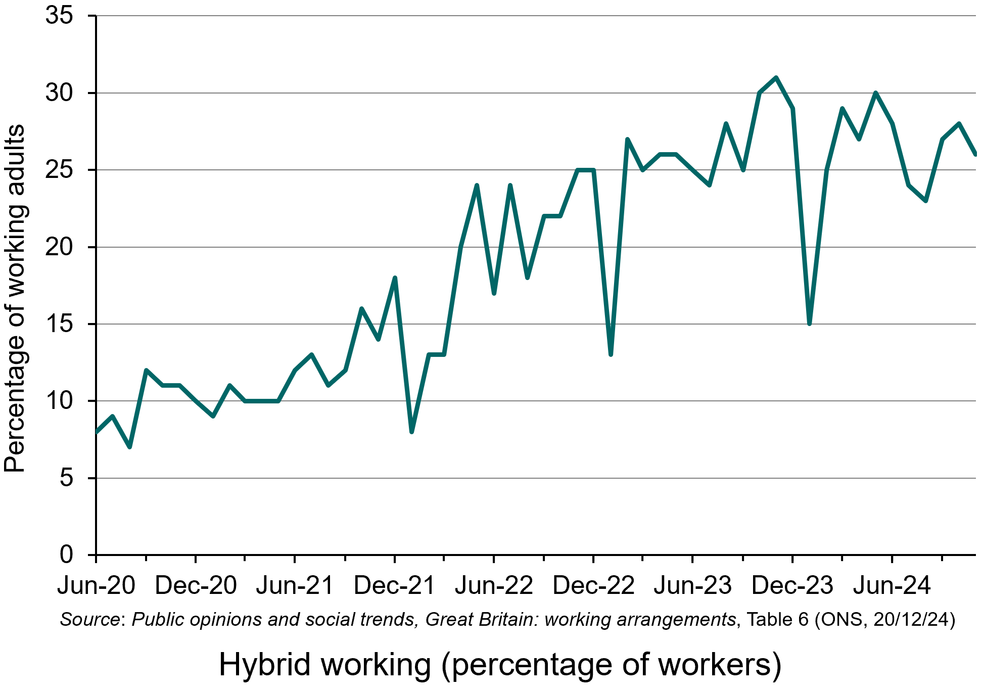
Today, this hybrid model, whereby workers work partly from home or local workspaces and partly in the office/factory/warehouse etc., has become the ‘new normal’ for around 26% of the working population in Great Britain – up from around 10% at the end of the national lockdowns in the Spring of 2021.
 Increasingly, however, employers who had introduced hybrid working are requiring their employees to return to the office, arguing that productivity and hence profits will rise as a result. Amazon is an example. Other employers, such as Asda, are increasing the time required in the office for hybrid workers.
Hybrid working had peaked at around 31% in November 2923 as the chart shows (click here for a PowerPoint). The chart is based on the December 20 database, Public opinions and social trends, Great Britain: working arrangements from the Office for National Statistics (see link under Data, below).
But why are some employers deciding that hybrid working is less profitable than working full time in the office. And does it apply to all employers and all employees or only certain types of firm and certain types of job?
The first thing to note is that hybrid work is more common among certain groups. These include older workers, parents, graduates and those with greater flexibility in scheduling their work, especially those in managerial or professional roles with greater flexibility. Certain types of work on the other hand do not lend themselves to hybrid work (or working completely from home, for that matter). Shop workers and those providing a direct service to customers, such as those working in the hospitality sector, cannot work remotely.
Benefits of hybrid working
For some employees and employers, hybrid working has brought significant benefits.
 For employees, less time and money is spent on commuting, which accounts for nearly an hour’s worth of the average worker’s daily time. According to the ONS survey, respondents spent an additional 24 minutes per day on sleep and rest and 15 minutes on exercise, sports and other activities that improved well-being compared to those who worked on-site. Working at home can make juggling work and home life easier, especially when workers can work flexible hours during the day, allowing them to fit work around family commitments.
Employers benefit from a healthier and more motivated staff who are more productive and less likely to quit. Hybrid work, being attractive to many workers, could allow employers to attract and retain talented workers. Also, employees may work longer hours if they are keen to complete a task and are not ‘clocking off’ at a particular time. Working from home allows workers to concentrate (unless distracted by other family members!).
By contrast, office working can be very inefficient, especially in open offices, where chatty colleagues can be distracting and it is difficult to concentrate. What is more, employees who are slightly unwell may continue working at home but may feel unable to commute to the office. If they did, they could spread their illness to other colleagues. Not allowing people to work from home can create a problem of ‘presenteeism’, where people feeling under the weather turn up to work but are unproductive.
One of the biggest benefits to employers of hybrid work is that costs can be saved by having smaller offices and by spending less on heating, lighting and facilities.
With hybrid working, time spent on site can be devoted to collaborative tasks, such as meetings with colleagues and customers/suppliers and joint projects where face-to-face discussion is required, or at least desirable. Tasks can also be completed that required specialist equipment or software not available at home.
Problems of hybrid working
So, if hybrid working has benefits for both employers and employees, why are some employers moving back to a system where employees work entirely on site?
 Some employers have found it hard to monitor and engage employees working from home. Workers may be easily distracted at home by other family members, especially if they don’t have a separate study/home office. People may feel detached from their co-workers on days they work from home. After a time, productivity may wane as workers find ways of minimising the amount of time actually working during declared work times.
Far from improving work-life balance, for some workers the boundaries between work and personal life can become blurred, which can erode the value of personal and family time. This can create a feeling of never escaping from work and be demotivating and reduce productivity. Employees may stay logged on longer and work evenings and weekends in order to complete tasks.
Unless carefully planned, on days when people do go into the office they might not work effectively. They may be less likely to have profitable ad hoc conversations with co-workers, and meetings may be harder to arrange. Misunderstandings and miscommunication can occur when some employees are in the office but others are at home.
Some employers have found that the problems of hybrid working in their organisations have outweighed the benefits and that productivity has fallen. In justifying its ending of hybrid working from 1 January 2025, Amazon CEO, Andy Jessy, wrote in a memo to staff in September 2024:
To address the … issue of being better set up to invent, collaborate, and be connected enough to each other and our culture to deliver the absolute best for customers and the business, we’ve decided that we’re going to return to being in the office the way we were before the onset of COVID. When we look back over the last five years, we continue to believe that the advantages of being together in the office are significant.1
But is the solution to do as Amazon is doing and to abandon hybrid working and have a mass ‘return to the office’?
Improving hybrid working
There are ways of making hybrid working more effective so that the benefits can be maximised and the costs minimised.
Given that there are specific benefits from home working and other specific benefits from working on-site, it would be efficient to allocate time between home and office to maximise these benefits. The optimum balance is likely to vary from employer to employer, job to job and individual to individual.
 Where work needs to be done in teams and where team meetings are an important element of that work, it would generally make sense for such meetings to be held in person, especially when there needs to be a lot of discussion. If the team requires a brief catch up, however, this may be more efficiently done online via Teams or Zoom.
Individual tasks, on the other hand, which don’t require consultation with colleagues or the use of specific workplace facilities, are often carried out more efficiently when there is minimum chance of interruption. For many workers, this would be at home rather than in an office – especially an open-plan office. For others without a protected work space at home or nearby, it might be better to come into the office.
The conclusion is that managers need to think carefully about the optimum distribution between home and office working and accept that a one-size-fits-all model may not be optimum for all types of job and all workers. Recognising the relative benefits and costs of working in different venues and over different hours may help to achieve the best balance, both for employers and for workers. A crucial element here is the appropriate use of incentives. Workers need to be motivated. Sometimes this may require careful monitoring, but often a more hands-off approach by management, with the focus more on output and listening to the concerns of workers, rather than on time spent, may result in greater productivity.
1Message from CEO Andy Jassy: Strengthening our culture and teams, Amazon News (16/9/24)
Articles
- Hybrid working is the ‘new normal’, according to ONS
Personnel Today, Jo Faragher (11/11/24)
- Hybrid working is here to stay but needs better managing
Business Live, Dylan Jones-Evans (18/11/24)
- The permanently imperfect reality of hybrid work
BBC: Worklife, Alex Christian (11/12/23)
- The diminishing returns of in-office mandates
BBC: Worklife, Alex Christian (12/6/24)
- The Advantages and Challenges of Hybrid Work
Gallup: Workplace, Ben Wigert and Jessica White (14/9/22)
- 9 Challenges of hybrid working and how you should tackle them
Manager Talks, Ankita (10/3/24)
- 5 Challenges of Hybrid Work — and How to Overcome Them
Harvard Business Review, Martine Haas (15/2/22)
- Post-Christmas blues as UK bosses try to turn back clock on hybrid working
The Guardian, Joanna Partridge (3/1/25)
- ‘It didn’t come as a surprise’: UK workers on being forced back into the office
The Guardian, Rachel Obordo (3/1/25)
- Amazon tells staff to get back to office five days a week
BBC News, Natalie Sherman (16/9/24)
- Inequality in flexible working dividing Britain into ‘two-tier workforce’
The Guardian, Joanna Partridge (27/1/25)
Data
Questions
- Why may hybrid working be better for (a) employees and (b) employers than purely home working or purely working in the office?
- Why are many firms deciding that workers who were formerly employed on a hybrid basis should now work entirely from the office?
- What types of job are better performed on site, or with only a small amount of time working from home?
- What types of job are better performed by working at home with just occasional days in the office?
- Does the profile of workers (by age, qualifications, seniority, experience, family commitments, etc) affect the likelihood that they will work from home at least some of the time?
- How would you set about measuring the marginal productivity of a worker working from home? Is it harder than measuring the marginal productivity of the same worker doing the same job but working in the office?
- How may working in the office increase network effects?
- How may behavioural economics help managers to understand the optimum balance of home and on-site working?
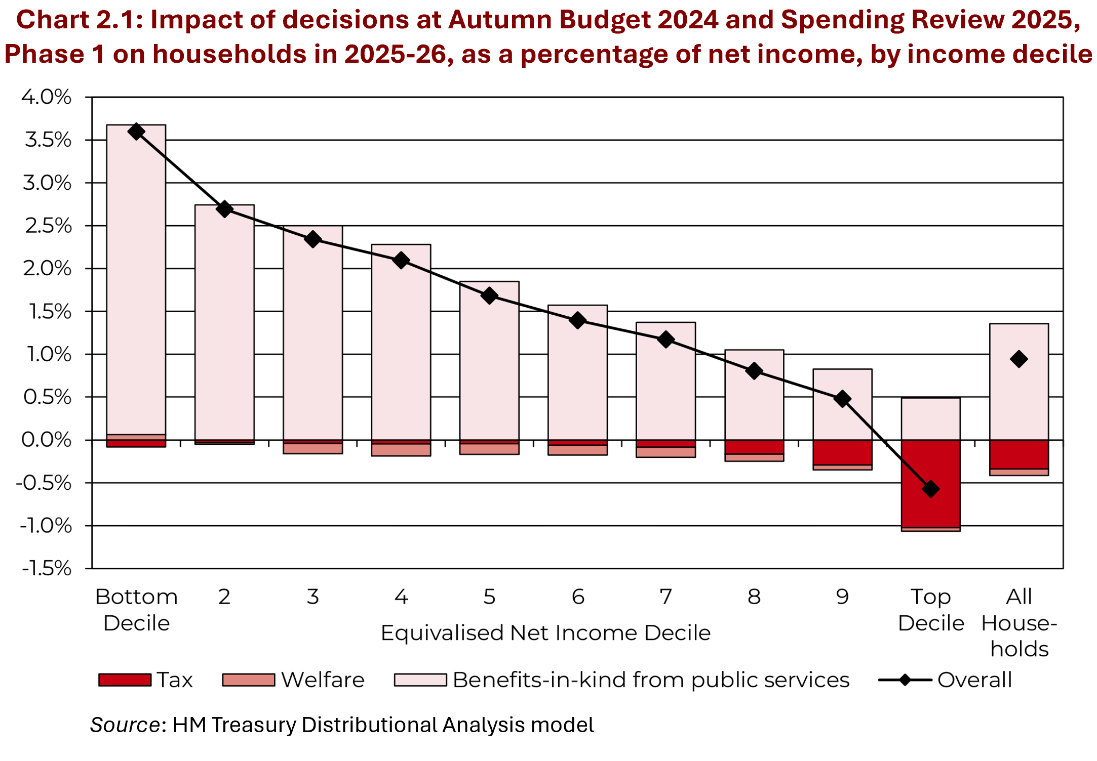 The first Budget of the new UK Labour government was announced on 30 October 2024. It contained a number of measures that will help to tackle inequality. These include extra spending on health and education. This will benefit households on lower incomes the most as a percentage of net income. Increases in tax, by contrast, will be paid predominantly by those on higher incomes. The Chart opposite (taken from the Budget Report) illustrates this. It shows that the poorest 10% will benefit from the largest percentage gain, while the richest 10% will be the only decile that loses.
But one of the major ways of tackling inequality and poverty was raising the minimum wage. The so-called ‘National Living Wage (NLW)’, paid to those aged 21 and over, will rise in April by 6.7% – from £11.44 to £12.41 per hour. The minimum wage paid to those aged 18 to 20 will rise 16.3% from £8.60 to £10.00 and for 16 and 17 year-olds and apprentices it will rise £18% from £6.40 to £7.55.
 It has been an objective of governments for several years to relate the minimum wage to the median wage. In 2015, the Conservative Government set a target of raising the minimum wage rate to 60 per cent of median hourly earnings by 2020. When that target was hit a new one was set to reach two-thirds of median hourly earnings by 2024.
The Labour government has set a new remit for the minimum wage (NLW). There are two floors. The first is the previously agreed one, that the NLW should be at least two-thirds of median hourly earnings; the second is that it should fully compensate for cost of living rises and for expected inflation up to March 2026. The new rate of £12.41 will meet both criteria. According to the Low Pay Commission, ‘Wages have risen faster than inflation over the past 12 months, and are forecast to continue to do so up to March 2026’. This makes the first floor the dominant one: meeting the first floor automatically meets the second.
How effective is the minimum wage in reducing poverty and inequality?
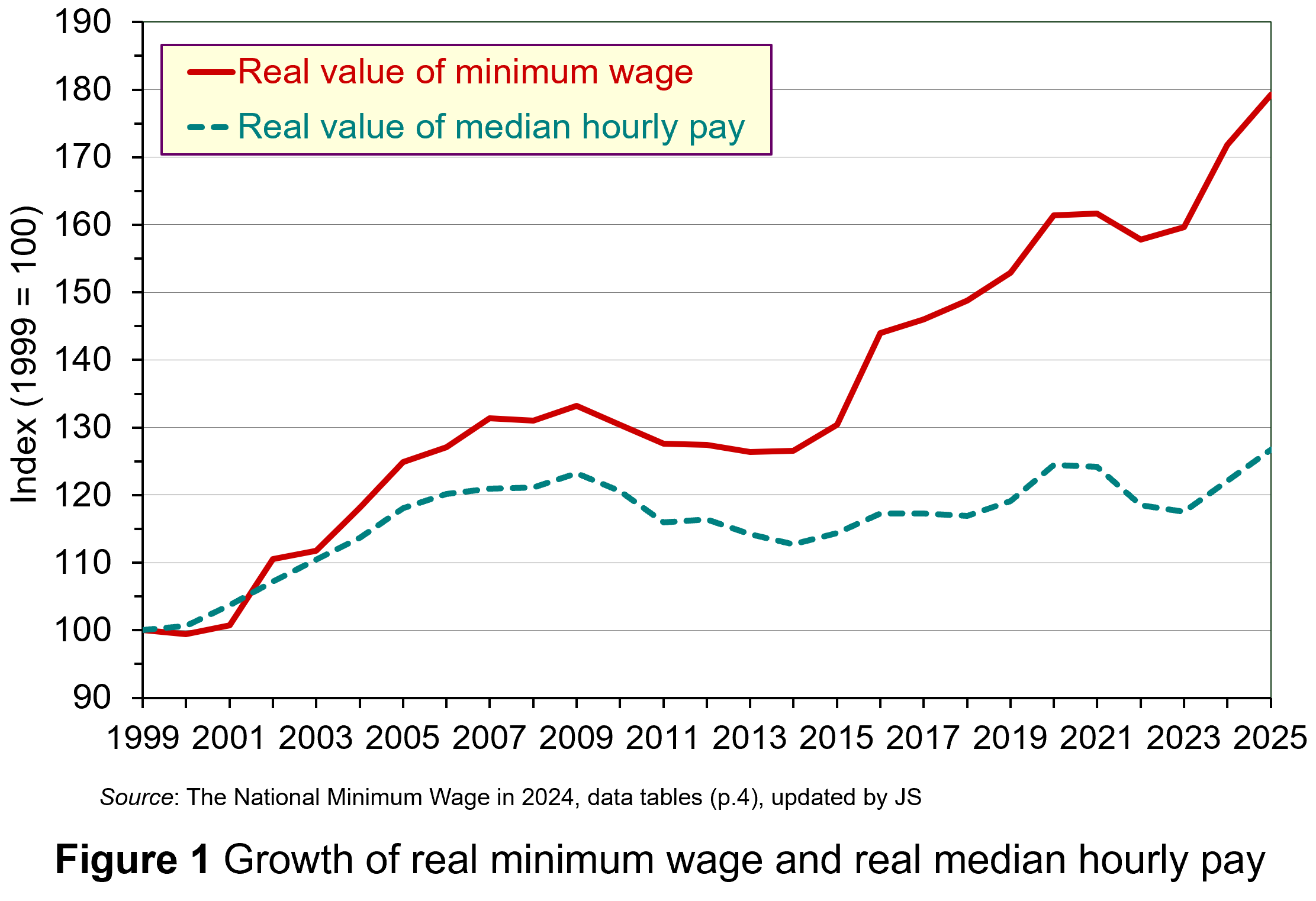 Figure 1 shows the growth in minimum wage rates since their introduction in 1999. The figures are real figures (i.e. after taking into account CPI inflation) and are expressed as an index, with 1999 = 100. The chart also shows the growth in real median hourly pay. (Click here for a Powerpoint.)
As you can see, the growth in real minimum wage rates has considerably exceeded the growth in real median hourly pay. This has had a substantial effect on raising the incomes of the poorest workers and thereby has helped to reduce poverty and inequality.
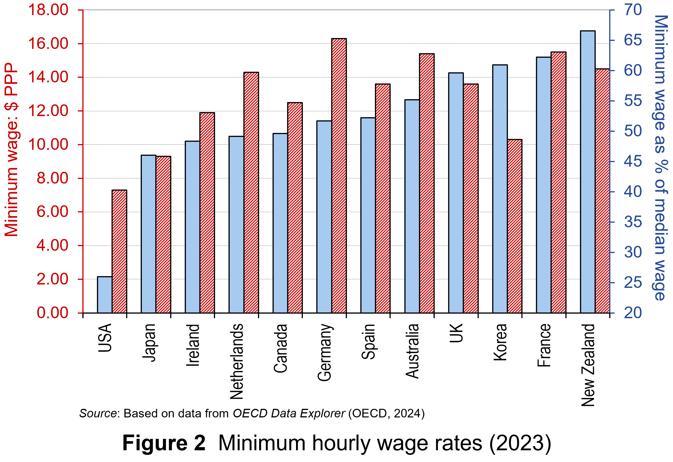 The UK minimum wage compares relatively favourably with other high-income economies. Figure 2 shows minimum wage rates in 12 high-income countries in 2023 – the latest year for which data are available. (Click here for a PowerPoint.) The red bars (striped) show hourly minimum wage rates in US dollars at purchasing-power parity (PPP) rates. PPP rates correct current exchange rates to reflect the purchasing power of each country’s currency. The blue bars (plain) show minimum wage rates as a percentage of the median wage rate. In 2023 the UK had the fourth highest minimum wage of the 12 countries on this measure (59.6%). As we have seen above, the 2025 rate is expected to be 2/3 of the median rate.
Minimum wages are just one mechanism for reducing poverty and inequality. Others include the use of the tax and benefit system to redistribute incomes. The direct provision of services, such as health, education and housing at affordable rents can make a significant difference and, as we have seen, have been a major focus of the October 2024 Budget.
The government has been criticised, however, for not removing the two-child limit to extra benefits in Universal Credit (introduced in 2017). The cap clearly disadvantages poor families with more than two children. What is more, for workers on Universal Credit, more than half of the gains from the higher minimum wages will lost because they will result in lower benefit entitlement. Also the freeze in (nominal) personal income tax allowances will mean more poor people will pay tax even with no rise in real incomes.
Effects on employment: analysis
A worry about raising the minimum wage rate is that it could reduce employment in firms already paying the minimum wage and thus facing a wage rise.
In the case of a firm operating in competitive labour and goods markets, the demand for low-skilled workers is relatively wage sensitive. Any rise in wage rates, and hence prices, by this firm alone would lead to a large fall in sales and hence in employment.
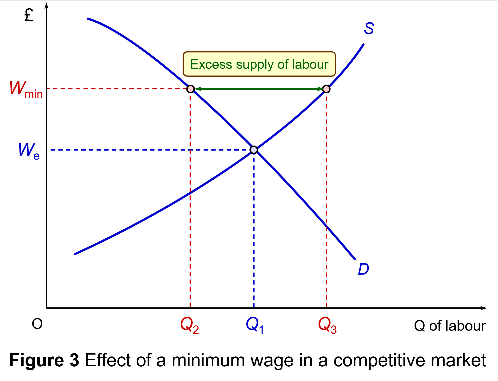 This is illustrated in Figure 3 (click here for a PowerPoint). Assume that the minimum wage is initially the equilibrium wage rate We. Now assume that the minimum wage is raised to Wmin. This will cause a surplus of labour (i.e. unemployment) of Q3 – Q2. Labour supply rises from Q1 to Q3 and the demand for labour falls from Q1 to Q2.
But, given that all firms face the minimum wage, individual employers are more able to pass on higher wages in higher prices, knowing that their competitors are doing the same. The quantity of labour demanded in any given market will not fall so much – the demand is less wage elastic; and the quantity of labour supplied in any given market will rise less – the supply is less wage elastic. Any unemployment will be less than that illustrated in Figure 3. If, at the same time, the economy expands so that the demand-for-labour curve shifts to the right, there may be no unemployment at all.
When employers have a degree of monopsony power, it is not even certain that they would want to reduce employment. This is illustrated in Figure 4: click here for a PowerPoint (you can skip this section if you are not familiar with the analysis).
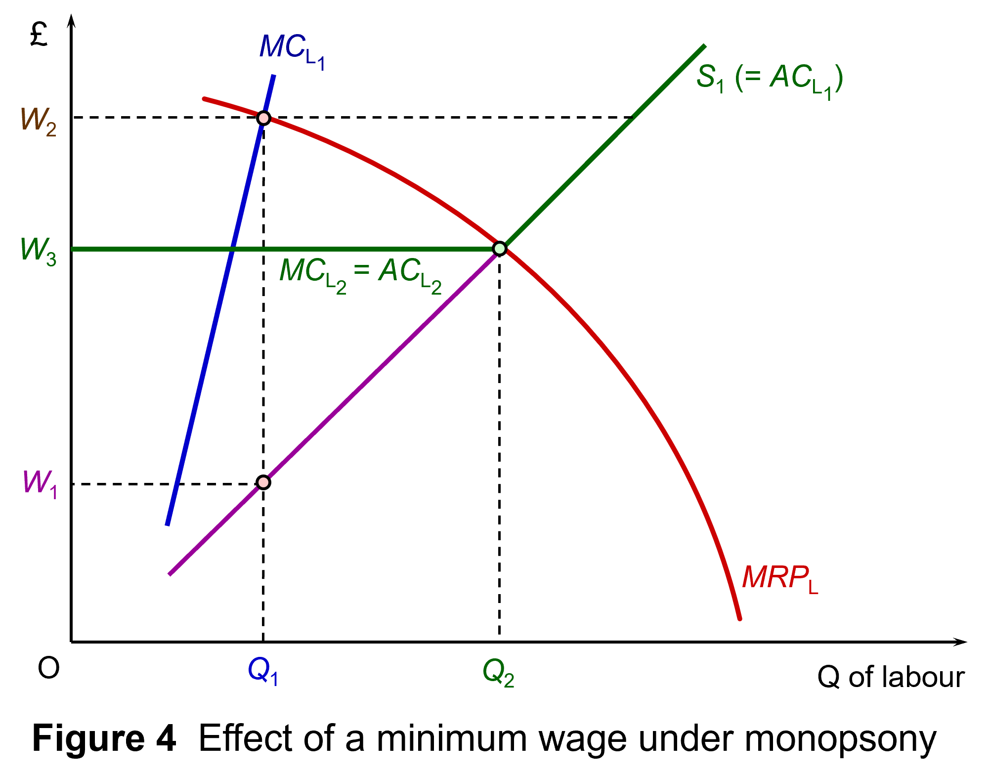 Assume initially that there is no minimum wage. The supply of labour to the monopsony employer is given by curve SL1, which is also the average cost of labour ACL1. A higher employment by the firm will drive up the wage; a lower employment will drive it down. This gives a marginal cost of labour curve of MCL1. Profit-maximising employment will be Q1, where the marginal cost of labour equals the marginal revenue product of labour (MRPL). The wage, given by the SL1 (=ACL1) line will be W1.
Now assume that there is a minimum wage. Assume also that the initial minimum wage is at or below W1. The profit-maximising employment is thus Q1 at a wage rate of W1.
The minimum wage can be be raised as high as W2 and the firm will still want to employ as many workers as at W1. The point is that the firm can no longer drive down the wage rate by employing fewer workers, and so the ACL1 curve becomes horizontal at the new minimum wage and hence will be the same as the MCL curve (MCL2 = ACL2). Profit-maximising employment will be where the MRPL curve equals this horizontal MCL curve. The incentive to cut its workforce, therefore, has been removed.
Again, if we extend the analysis to the whole economy, a rise in the minimum wage will be partly passed on in higher prices or stimulate employers to increase labour productivity. The effect will be to shift the (MRPL) curve upwards to the right, thereby allowing the firm to pass on higher wages and reducing any incentive to reduce employment.
Effects on employment: evidence
There is little evidence that raising the minimum wage in stages will create unemployment, although it may cause some redeployment. In the Low Pay Commission’s 2019 report, 20 years of the National Minimum Wage (see link below), it stated that since 2000 it had commissioned more than 30 research projects looking at the NMW’s effects on hours and employment and had found no strong evidence of negative effects. Employers had adjusted to minimum wages in various ways. These included reducing profits, increasing prices and restructuring their business and workforce.
Along with our commissioned work, other economists have examined the employment effects of the NMW in the UK and have for the most part found no impact. This is consistent with international evidence suggesting that carefully set minimum wages do not have noticeable employment effects. While some jobs may be lost following a minimum wage increase, increasing employment elsewhere offsets this. (p.20)
There is general agreement, however, that a very large increase in minimum wages will impact on employment. This, however, should not be relevant to the rise in the NLW from £11.44 to £12.41 per hour in April 2025, which represents a real rise of around 4.5%. This at worst should have only a modest effect on employment and could be offset by economic growth.
 What, however, has concerned commentators more is the rise in employers’ National Insurance contributions (NICs) that were announced in the Budget. In April 2025, the rate will increase from 13.8% to 15%. Employers’ NICs are paid for each employee on all wages above a certain annual threshold. This threshold will fall in April from £9100 to £5000. So the cost to an employer of an employee earning £38 000 per annum in 2024/25 would be £38 000 + ((£38 000 – £9100) × 0.138) = £41 988.20. For the year 2025/26 it will rise to £38 000 + ((£38 000 – £5000) × 0.15) = £42 950. This is a rise of 2.29%. (Note that £38 000 will be approximately the median wage in 2025/26.)
However, for employees on the new minimum wage, the percentage rise in employer NICs will be somewhat higher. A person on the new NLW of £12.41, working 40 hours per week and 52 weeks per year (assuming paid holidays), will earn an annual wage of £25 812.80. Under the old employer NIC rates, the employer would have paid (£25 812.80 + (£25 812.80 – £9100) × 0.138) = £28 119.17. For the year 2025/26, it will rise to £25 812.80 + ((£25 812.80 – £5000) × 0.15) = £28 934.72. This is a rise of 2.90%.
This larger percentage rise in employers’ wage costs for people on minimum wages than those on median wages, when combined with the rise in the NLW, could have an impact on the employment of those on minimum wages. Whether it does or not will depend on how rapid growth is and how much employers can absorb the extra costs through greater productivity and/or passing on the costs to their customers.
Articles
- National Living Wage to increase to £12.21 in April 2025
Low Pay Commission, Press Release (29/10/24)
- Rachel Reeves hands low-paid a £1,400 boost as minimum wage to rise by 6.7%
Independent, Archie Mitchell and Millie Cooke (31/10/24)
- Minimum wage to rise to £12.21 an hour next year
BBC News, Michael Race (29/10/24)
- What Labour’s first budget means for wages, taxes, business, the NHS and plans to grow the economy – experts explain
The Conversation, Rachel Scarfe et al. (30/10/24)
- The two-child limit: poverty, incentives and cost
Institute for Fiscal Studies, Eduin Latimer and Tom Waters (17/6/24)
UK Government reports and information
Data
Questions
- How is the October 2024 Budget likely to affect the distribution of income?
- What are the benefits and limitations of statutory minimum wages in reducing (a) poverty and (b) inequality?
- Under what circumstances will a rise in the minimum wage lead or not lead to an increase in unemployment?
- Find out what is meant by the UK Real Living Wage (RLW) and distinguish it from the UK National Living Wage (NLW). Why is the RLW higher?
- Why is the median wage rather than the mean wage used in setting the NLW?
 In recent months there has been growing uncertainty across the global economy as to whether the US economy was going to experience a ‘hard’ or ‘soft landing’ in the current business cycle – the repeated sequences of expansion and contraction in economic activity over time. Announcements of macroeconomic indicators have been keenly anticipated for signals about how quickly the US economy is slowing.
Such heightened uncertainty is a common feature of late-cycle slowing economies, but uncertainty now has been exacerbated because it has been a while since developed economies have experienced a business cycle like the current one. The 21st century has been characterised by low inflation, low interest rates and recessions caused by various types of crises – a stock market crisis (2001), a banking crisis (2008) and a global pandemic (2020). In contrast, the current cycle is a throwback to the 20th century. The high inflation and the ensuing increases in interest rates have produced a business cycle which echoes the 1970s. Therefore, few investors have experience of such economic conditions.
The focus for investors during this stage of the cycle is when the slowing economy will reach the minimum. They will also be concerned with the depth of the slowdown: will there still be some growth in income, albeit low; or will the trough be severe enough to produce a recession, and, if so, how deep? Given uncertainty around the length and magnitude of business cycles, this leads to greater risk aversion among investors. This affects reactions to announcements of leading and lagging macroeconomic indicators.
This blog examines what sort of economic conditions we should expect in a late-cycle economy. It analyses the impact this has had on investor behaviour and the ensuing dynamics observed in financial markets in the USA.
The Business Cycle
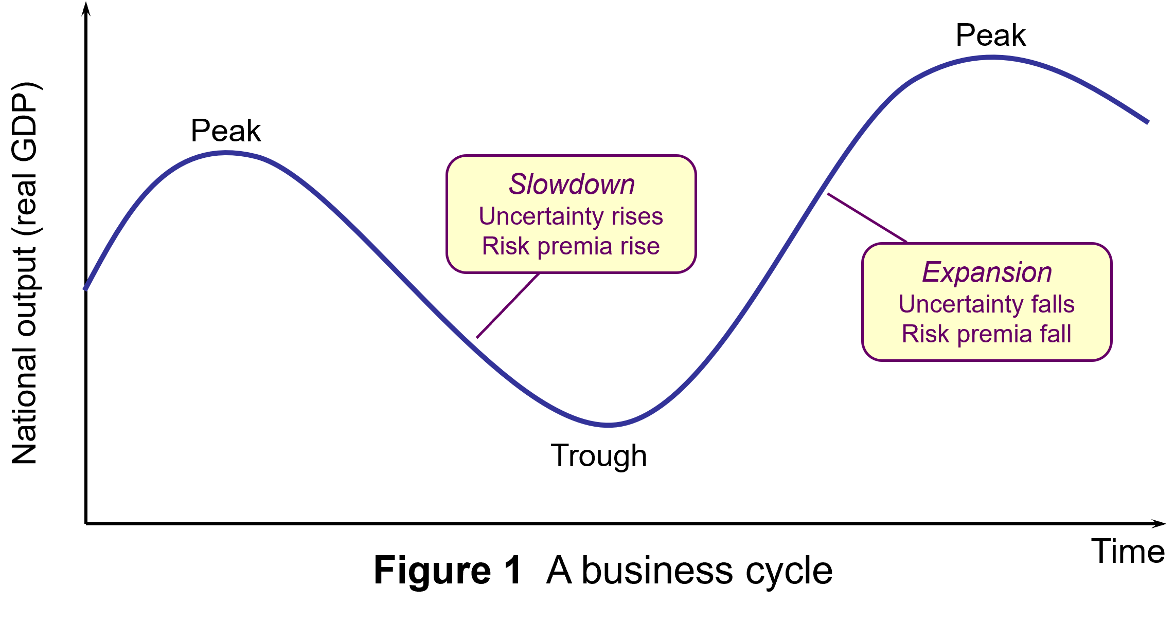
The business cycle refers to repeated sequences of expansion and contraction (or slowdown) in economic activity over time. Figure 1 illustrates a typical cycle. Typically, these sequences include four main stages. In each one there are different effects on consumer and business confidence:
- Expansion: During this stage, the economy experiences growth in GDP, with incomes and consumption spending rising. Business and consumer confidence are high. Unemployment is falling.
- Peak: This is the point at which the economy reaches its maximum output, but growth has ceased (or slowed). At this stage, inflationary pressures peak as the economy presses against potential output. This tends to result in tighter monetary policy (higher interest rates).
- Slowdown: The higher interest rates raise the cost of borrowing and reduce consumption and investment spending. Consumption and incomes both slow or fall. (Figure 1 illustrates the severe case of falling GDP (negative growth) in this stage.) Unemployment starts rising.
- Trough: This is the lowest point of the cycle, where economic activity bottoms out and the economy begins to recover. This can be associated with slow but still rising national income (a soft landing) or national income that has fallen (a hard landing, as shown in Figure 1).
While business cycles are common enough to enable such characterisation of their temporal pattern, their length and magnitude are variable and this produces great uncertainty, particularly when cycles approach peaks and troughs.
 As an economy’s cycle approaches a trough, such as US economy’s over the past few months, uncertainty is exacerbated. The high interest rates used to tackle inflation will have increased borrowing costs for businesses and consumers. Access to credit may have become more restricted. Profit margins are reduced, especially for industrial sectors sensitive to the business cycle, reducing expected cash flows.
The combination of these factors can increase the risk of a recession, producing greater volatility in financial markets. This manifests itself in increased risk aversion among investors.
Utility theory suggests that, in general, investors will exhibit loss aversion. This means that they do not like bearing risk, fearing that the return from an investment may be less than expected. In such circumstances, investors need to be compensated for bearing risk. This is normally expressed in terms of expected financial return. To bear more risk, investors require higher levels of return as compensation.
As perceptions of risk change through the business cycle, so this will change the return investors will require from the financial instruments they hold. Perceived higher risk raises the return investors will require as compensation. Conversely, lower perceived risk decreases the return investors expect as compensation.
Investors’ expected rate of return is manifested in the discount rate that they use to value the anticipated cash flows from financial instruments in discounted cash flow (DCF) analysis. Equation 1 is the algebraic expression of the present-value discounted series of cash flows for financial instruments:

Where:
V = present value
C = anticipated cash flows in each of time periods 1, 2, 3, etc.
r = expected rate of return
For fixed-income debt securities, the cash flow is constant, while for equity securities (shares), expectations regarding cash flows can change.
Slowing economies and risk aversion
 In a slowing economy, with great uncertainty about the scale and timing of the bottom of the cycle, investors become more risk averse about the prospects of firms. This this leads to higher risk premia for financial instruments sensitive to a slowdown in economic activity.
This translates into a higher expected return and higher discount rate used in the valuation of these instruments (r in equation 1). This produces decreases in perceived value, decreased demand and decreased prices for these financial instruments. This can be observed in the market dynamics for these instruments.
First, there may be a ‘flight to safety’. Investors attach a higher risk premium to risker financial instruments, such as equities, and seek a ‘safe-haven’ for their wealth. Therefore, we should observe a reorientation from more risky to less risky assets. Demand for equities falls, while demand for safer assets, such as government bonds and gold, rises.
There is some evidence for this behaviour as uncertainty about the US economic outlook has increased. Gold, long seen as a hedge against market decline, is at record highs. US Government bond prices have risen too.
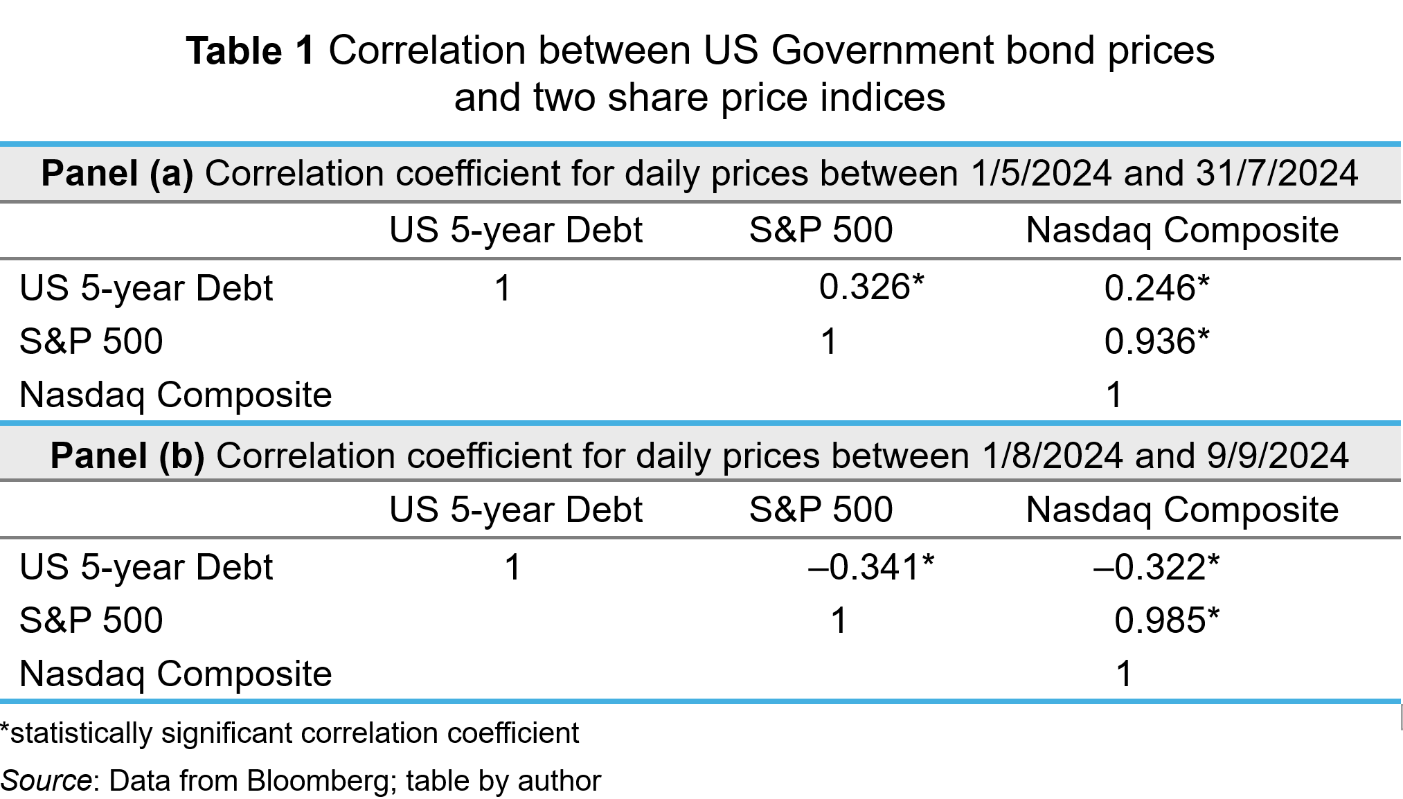
To analyse whether this may be a flight to safety, I analysed the correlation between the daily US government bond price (5-year Treasury Bill) and share prices represented by the two more significant stock market indices in the USA: the S&P 500 and the Nasdaq Composite. I did this for two different time periods. Table 1 shows the results. Panel (a) shows the correlation coefficients for the period between 1 May 2024 and 31 July 2024; Panel (b) shows the correlation coefficients for the period between 1 August 2024 and 9 September 2024.

In the period between May and July 2024, the 5-year Treasury Bill and share price indices had significantly positive correlations. When share prices rose, the Treasury Bill’s price rose; when share prices fell, the bill’s price fell. During that period, expectations about falling interest rates dominated valuations and that effected the valuations of all financial instruments in the same way – lower expected interest rates reduce the opportunity cost of holding instruments and reduces the expected rates of return. Hence, the discount rate applied to cash flows is reduced, and present value rises. The opposite happens when macroeconomic indicators suggest that interest rates will stay high (ceteris paribus).
As the summer proceeded, worries about a ‘hard landing’ began to concern investors. A weak jobs report in early August particularly exercised markets, producing a ‘flight to safety’. Greater risk aversion among investors meant that they expect a higher return from equities. This reduced perceived value, reducing demand and price (ceteris paribus). To insulate themselves from higher risk, investors bought safer assets, like government bonds, thereby pushing up their prices. This behaviour was consistent with the significant negative correlation observed between US government debt prices and the S&P 500 and Nasdaq indices in Panel (b).
Another signal of increased risk aversion among investors is ‘sector rotation’ in their equity portfolios. Increased risk aversion among investors will lead them to divest from ‘cyclical’ companies. Such companies are in industrial sectors which are more sensitive to the changing economic conditions across the business cycle – consumer discretionary and communication services sectors, for example. To reduce their exposure to risk, investors will switch to ‘defensive’ sectors – those less sensitive to the business cycle. Examples include consumer staples and utility sectors.
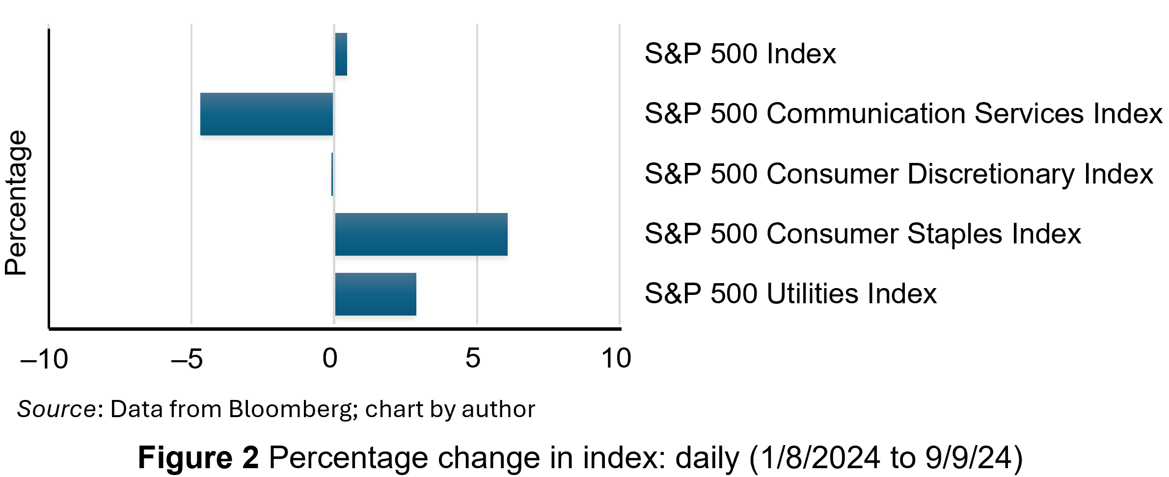
Cyclical sectors will suffer a greater adverse impact on their cash flows and risk in a slowing economy. Consequently, investors expect higher return as compensation. This reduces the value of those shares. Demand for them falls, depressing their price. In contrast, defensive sectors will be valued more. They will see an increase in demand and price. This sector rotation seems to have happened in August (2024). Figure 2 shows the percentage change between 1 August and 9 September 2024 in the S&P 500 index and four sector indices, comprising companies from the communication services, consumer discretionary, consumer staples and utilities sectors.

Overall, the S&P 500 index was slightly higher, as shown by the first bar in the chart. However, while the cyclical sectors experienced decreases in their share prices, particularly communication services, the defensive companies experienced large price increases – nearly 3% for utilities and over 6% for consumer staples.
Conclusion
Economies experience repeated sequences of expansion and contraction in economic activity over time. At the moment, the US economy is approaching the end of its current slowing phase. Increased uncertainty is a common feature of late-cycle economies and this manifests itself in heightened risk aversion among investors. This produces certain dynamics which have been observable in US debt and equity markets. This includes a ‘flight to safety’, with investors divesting risky financial instruments in favour of safer ones, such as US government debt securities and gold. Also, investors have been reorientating their equity portfolios away from cyclicals and towards defensive securities.
Articles
- America’s recession signals are flashing red. Don’t believe them
The Economist (22/8/24)
- The most well-known recession indicator stopped flashing red, but now another one is going off
CNN, Elisabeth Buchwald (13/9/24)
- World’s largest economy will still achieve soft landing despite rising unemployment, most analysts believe
Financial Times, Claire Jones, Delphine Strauss and Martha Muir (6/8/24)
- We’re officially on slowdown watch
Financial Times, Robert Armstrong and Aiden Reiter (30/8/24)
- Anatomy of a rout
Financial Times, Robert Armstrong and Aiden Reiter (6/8/24)
- Reasons why investors need to prepare for a US recession
Financial Times, Peter Berezin (5/9/24)
- Business Cycle: What It Is, How to Measure It, and Its 4 Phases
Investopedia, Lakshman Achuthan (6/6/24)
- Risk Averse: What It Means, Investment Choices, and Strategies
Investopedia, James Chen (5/8/24)
Data
Questions
- What is risk aversion? Sketch an indifference curve for a risk-averse investor, treating expected return and risk as two-characteristics of a financial instrument.
- Show what happens to the slope of the indifference curve if the investor becomes more risk averse.
- Using demand and supply analysis, illustrate and explain the impact of a flight to safety on the market for (i) company shares and (ii) US government Treasury Bills.
- Use economic theory to explain why the consumer discretionary sector may be more sensitive than the consumer staples sector to varying incomes across the economic cycle.
- Research the point of the economic cycle that the US economy has reached as you read this blog. What is the relationship between bond and equity prices? Which sectors have performed best in the stock market?
 In a blog in October 2024, we looked at global uncertainty and how it can be captured in a World Uncertainty Index. The blog stated that ‘We continue to live through incredibly turbulent times. In the past decade or so we have experienced a global financial crisis, a global health emergency, seen the UK’s departure from the European Union, and witnessed increasing levels of geopolitical tension and conflict’.
  The World Uncertainty Index (WUI) tracks uncertainty around the world by applying a form of text mining known as ‘term frequency’ to the country reports produced by the Economist Intelligence Unit (EIU). The words searched for are ‘uncertain’, ‘uncertainty’ and ‘uncertainties’ and the number of times they occur as percentage of the total words is recorded. To produce the WUI this figure is then multiplied by 1m. A higher WUI number indicates a greater level of uncertainty.
 The second chart shows the World Trade Uncertainty Index (WTUI), published on the same site as the WUI (click here for a PowerPoint). The method adopted in its construction therefore mirrors that for the WUI but counts the number of times in EIU country reports ‘uncertainty’ is mentioned within proximity to a word related to trade, such as ‘protectionism’, ‘NAFTA’, ‘tariff’, ‘trade’, ‘UNCTAD’ or ‘WTO.’
  In a blog from March 2023 (reproduced below), we saw how there has been growing pressure around the world for employers to move to a four-day week. Increasing numbers of companies have adopted the model of 80% of the hours for 100% of the pay.
 Since the financial crisis of 2007–8, the growth in UK productivity has been sluggish. This is illustrated in the chart, which looks at the production industries: i.e. it excludes services, where average productivity growth tends to be slower. The chart has been updated to 2024 Q2 – the latest data available. (Click
  Productivity in the UK is lower than in many other competitor countries.
  The model adopted varied across companies, depending on what was seen as most suitable for them. Some gave everyone Friday off; others let staff choose which day to have off; others let staff work 80% of the hours on a flexible basis.
 During the pandemic, most people who were not furloughed were forced to work from home. After lockdown restrictions were lifted, many employers decided to continue with people working remotely, at least for some of the time.
 Increasingly, however, employers who had introduced hybrid working are requiring their employees to return to the office, arguing that productivity and hence profits will rise as a result. Amazon is an example. Other employers, such as Asda, are increasing the time required in the office for hybrid workers.
 For employees, less time and money is spent on commuting, which accounts for nearly an hour’s worth of the average worker’s daily time. According to the ONS survey, respondents spent an additional 24 minutes per day on sleep and rest and 15 minutes on exercise, sports and other activities that improved well-being compared to those who worked on-site. Working at home can make juggling work and home life easier, especially when workers can work flexible hours during the day, allowing them to fit work around family commitments.
  Some employers have found it hard to monitor and engage employees working from home. Workers may be easily distracted at home by other family members, especially if they don’t have a separate study/home office. People may feel detached from their co-workers on days they work from home. After a time, productivity may wane as workers find ways of minimising the amount of time actually working during declared work times.
 Where work needs to be done in teams and where team meetings are an important element of that work, it would generally make sense for such meetings to be held in person, especially when there needs to be a lot of discussion. If the team requires a brief catch up, however, this may be more efficiently done online via Teams or Zoom.
  The first Budget of the new UK Labour government was announced on 30 October 2024. It contained a number of measures that will help to tackle inequality. These include extra spending on health and education. This will benefit households on lower incomes the most as a percentage of net income. Increases in tax, by contrast, will be paid predominantly by those on higher incomes. The Chart opposite (taken from the
  It has been an objective of governments for several years to relate the minimum wage to the median wage. In 2015, the Conservative Government set a target of raising the minimum wage rate to 60 per cent of median hourly earnings by 2020. When that target was hit a new one was set to reach two-thirds of median hourly earnings by 2024.
 Figure 1 shows the growth in minimum wage rates since their introduction in 1999. The figures are real figures (i.e. after taking into account CPI inflation) and are expressed as an index, with 1999 = 100. The chart also shows the growth in real median hourly pay. (Click
  The UK minimum wage compares relatively favourably with other high-income economies. Figure 2 shows minimum wage rates in 12 high-income countries in 2023 – the latest year for which data are available. (Click
  This is illustrated in Figure 3 (click
  Assume initially that there is no minimum wage. The supply of labour to the monopsony employer is given by curve SL1, which is also the average cost of labour ACL1. A higher employment by the firm will drive up the wage; a lower employment will drive it down. This gives a marginal cost of labour curve of MCL1. Profit-maximising employment will be Q1, where the marginal cost of labour equals the marginal revenue product of labour (MRPL). The wage, given by the SL1 (=ACL1) line will be W1.
  What, however, has concerned commentators more is the rise in employers’ National Insurance contributions (NICs) that were announced in the Budget. In April 2025, the rate will increase from 13.8% to 15%. Employers’ NICs are paid for each employee on all wages above a certain annual threshold. This threshold will fall in April from £9100 to £5000. So the cost to an employer of an employee earning £38 000 per annum in 2024/25 would be £38 000 + ((£38 000 – £9100) × 0.138) = £41 988.20. For the year 2025/26 it will rise to £38 000 + ((£38 000 – £5000) × 0.15) = £42 950. This is a rise of 2.29%. (Note that £38 000 will be approximately the median wage in 2025/26.)
 In recent months there has been growing uncertainty across the global economy as to whether the US economy was going to experience a ‘hard’ or ‘soft landing’ in the current business cycle – the repeated sequences of expansion and contraction in economic activity over time. Announcements of macroeconomic indicators have been keenly anticipated for signals about how quickly the US economy is slowing.
 As an economy’s cycle approaches a trough, such as US economy’s over the past few months, uncertainty is exacerbated. The high interest rates used to tackle inflation will have increased borrowing costs for businesses and consumers. Access to credit may have become more restricted. Profit margins are reduced, especially for industrial sectors sensitive to the business cycle, reducing expected cash flows.
 In a slowing economy, with great uncertainty about the scale and timing of the bottom of the cycle, investors become more risk averse about the prospects of firms. This this leads to higher risk premia for financial instruments sensitive to a slowdown in economic activity.