 In a blog in October 2024, we looked at global uncertainty and how it can be captured in a World Uncertainty Index. The blog stated that ‘We continue to live through incredibly turbulent times. In the past decade or so we have experienced a global financial crisis, a global health emergency, seen the UK’s departure from the European Union, and witnessed increasing levels of geopolitical tension and conflict’.
Since then, Donald Trump has been elected for a second term and has introduced sweeping tariffs. What is more, the tariffs announced on so-called ‘Liberation Day‘ have not remained fixed, but have fluctuated with negotiations and threatened retaliation. The resulting uncertainty makes it very hard for businesses to plan and many have been unwilling to commit to investment decisions. The uncertainty has been compounded by geopolitical events, such as the continuing war in Ukraine, the war in Gaza and the June 13 Israeli attack on Iran.
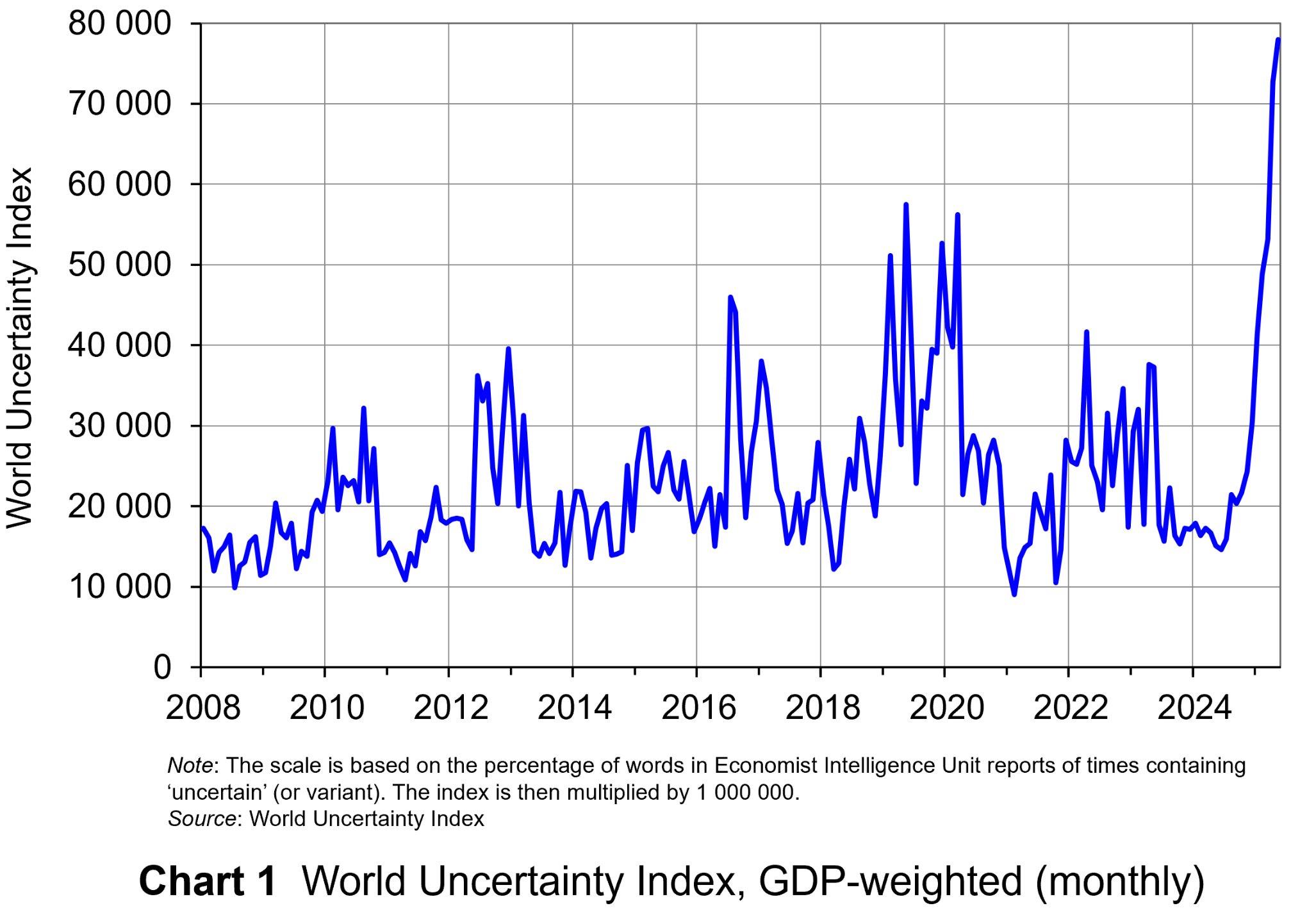 The World Uncertainty Index (WUI) tracks uncertainty around the world by applying a form of text mining known as ‘term frequency’ to the country reports produced by the Economist Intelligence Unit (EIU). The words searched for are ‘uncertain’, ‘uncertainty’ and ‘uncertainties’ and the number of times they occur as percentage of the total words is recorded. To produce the WUI this figure is then multiplied by 1m. A higher WUI number indicates a greater level of uncertainty.
The monthly global average WUI is shown in Chart 1 (click here for a PowerPoint). It is based on 71 countries. Since 2008 the WUI has averaged a little over 23 000: i.e. 2.3 per cent of the text in EIU reports contains the word ‘uncertainty’ or a close variant. In May 2025, it was almost 79 000 – the highest since the index was first complied in 2008. The previous highest was in March 2020, at the start of the COVID-19 outbreak, when the index rose to just over 56 000.
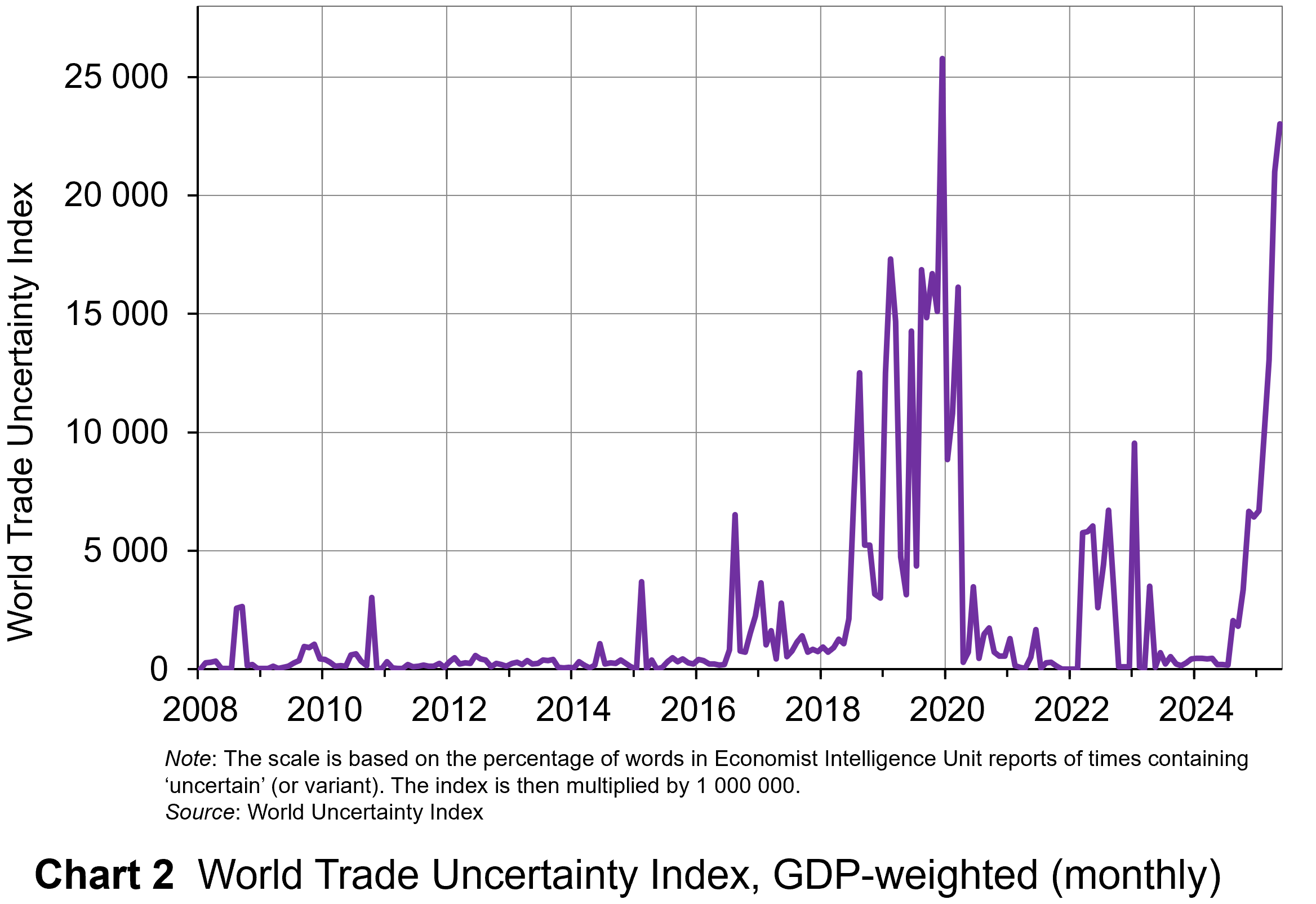 The second chart shows the World Trade Uncertainty Index (WTUI), published on the same site as the WUI (click here for a PowerPoint). The method adopted in its construction therefore mirrors that for the WUI but counts the number of times in EIU country reports ‘uncertainty’ is mentioned within proximity to a word related to trade, such as ‘protectionism’, ‘NAFTA’, ‘tariff’, ‘trade’, ‘UNCTAD’ or ‘WTO.’
The chart shows that in May 2025, the WTUI had risen to just over 23 000 – the second highest since December 2019, when President Trump imposed a new round of tariffs on Chinese imports and announced that he would restore steel tariffs on Brazil and Argentina. Since 2008, the WTUI has averaged just 2228.
It remains to be seen whether more stability in trade relations and geopolitics will allow WUI and WUTI to decline once more, or whether greater instability will simply lead to greater uncertainty, with damaging consequences for investment and also for consumption and employment.
Articles
Uncertainty Indices
Questions
- Explain what is meant by ‘text mining’. What are its strengths and weaknesses in assessing business, consumer and trade uncertainty?
- Explain how the UK Monthly EPU Index is derived.
- Why has uncertainty increased so dramatically since the start of 2025?
- Compare indices based on text mining with confidence indices.
- Plot consumer and business/industry confidence indicators for the past 24 months, using EC data. Do they correspond with the WUI?
- How may uncertainty affect consumers’ decisions?
For a while now, debate has raged over how to revive the fortunes of the London Stock Exchange (LSE). Since the 2008 financial crisis, the market has suffered a lack of investment, poor liquidity and low performance. This has produced a moribund financial market which has become unattractive to both investors and companies. Returns from the UK market lag international competitors, particularly the USA (see the chart).
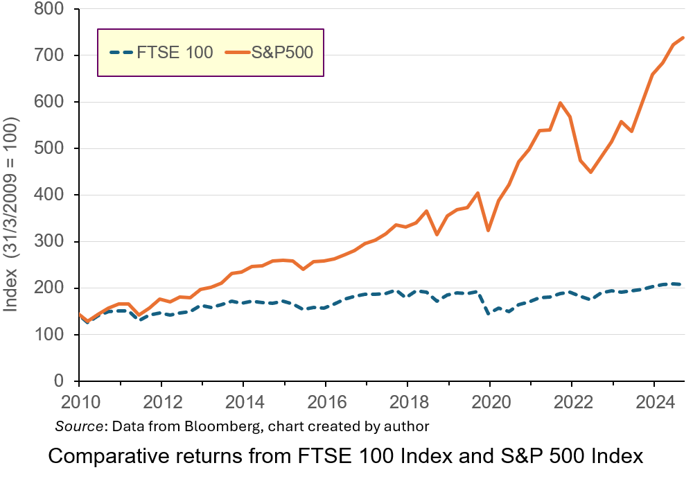
Investment in the S&P 500 Index over the period would have produced annualised rates of return of 14.35%, more than double that from the FTSE 100 Index. Part of this underperformance is due to the industrial mix of the listed companies: low-growth energy and mining compared to the high-growth technology sectors in the USA. This has led to the perception that London is not a place for firms to list, particularly those in high-growth sectors.
In 2024, 88 companies choose to delist or transfer their primary listing elsewhere. Only 18 took their place. Several big companies from a range of industries, including Ashtead, Flutter and CRH have transferred their primary listing to New York or have plans to do so.
 The new Labour government views stimulating higher levels of investment though the London market as an important element in its drive to boost productivity and growth in the UK. Recently, it has been reported that investment institutions have been lobbying the UK government to reduce significantly the tax-free allowance for Cash Individual Savings Accounts (ISAs) as a way to encourage more of UK households’ savings to be channelled through the UK stock market.
Currently, UK savers can save up to £20 000 annually into ISAs without paying tax on the interest earned. This can be held solely in Cash ISAs, or in a combination of Cash plus Stocks and Shares ISAs. The tax-free instruments which were introduced by a Labour government in 1999 to encourage higher savings have proved immensely popular. Data from Paragon Bank indicate that over £350 billion are held in these accounts. However, under the new proposals, the amount which would be allowed to be saved as cash has been rumoured to be cut to £4000 per year, with the hope that some of it will be invested in the UK stock market.
The proposals have proved controversial, with high-profile figures voicing opposition. In this blog, we’ll analyse the reasons behind the proposal and discuss whether it will have the desired effect of stimulating higher levels of investment. We’ll also discuss other proposed policies for making the LSE a more effective channel for investment flows to boost economic growth.
Stock markets and the saving and investment channel
 The main reason for the proposed ISA change is to encourage more investment in the UK stock market. By reducing the amount which can be saved in Cash ISAs, the government hopes to encourage savers to invest in Stocks and Shares ISAs instead, particularly ones linked to the UK market. This would increase the amount of finance capital in the market, thereby boosting its liquidity. This would then make it an attractive place for young, vibrant UK and foreign companies to list.
An active, liquid secondary market in shares is important to attract firms to list on stock exchanges by issuing shares to outside investors. Traditionally, this channel has been important to the growth and development of firms.
Existing savings in Cash ISAs are deposited with financial institutions such as banks and building societies. Through the credit-creation process such funds can be used to finance productive investment. In countries like the UK, lending by financial institutions is an important way that investment is financed, particularly for small and medium-sized enterprises. However, scale limits, regulatory restrictions and the need to diversify lending properly means that there are limits to the financing available for company investment through these institutions.
Capital markets like the LSE are intended to meet these larger-scale requirements. Financial claims, such as debt and equity, are divided into atomised instruments and sold to outside investors to fund investment and business growth.
 Further, the desire for a capital injection to finance growth is not the only reason that firms seek stock market listings. Founders of companies may have a lot of wealth invested in the equity of their firms. Selling some of their equity to outside investors through a stock market listing is a way of diversifying their wealth. However, if they are to maximise the potential sale price, there must be an active, liquid secondary market to encourage investors to buy shares in the primary market.
Proponents of reform want to encourage a greater appetite for risk among UK investors, which will produce more savings being channelled through the LSE.
One issue is whether savers will respond in the way anticipated and channel more funds through the UK stock market. Many savers like the security of Cash ISAs. Such vehicles offer a low-risk/low-return combination, which savers like because the tax benefits boost returns. A survey by the Nottingham Building Society found that a substantial number of Cash ISA savers are concerned that the proposed changes could affect their ability to save for important financial goals, such as buying a house or building an emergency fund. Higher-risk Stocks and Shares ISAs are not suitable for such savings because of the potential to lose the initial amount invested. Many may not be prepared to do so and one-third suggested they would save less overall.
According to the survey, only 38% of Cash ISA holders said they would consider investing in Stocks and Shares ISAs if the Cash ISA allowance were reduced. It may be difficult to alter such risk-averse preferences given the average amount saved through ISAs and demographics. In 2022/23, the average amount subscribed to ISAs was £5000. This does not suggest that average households have a significant surplus of cash that they may want to investment at a high risk through the stock market. Indeed, many may want to have access to the cash at short notice and so are not prepared to forgo liquidity for the time needed to accrue the benefits of compounding which stock market investing produces.
 Demographics may also play a role in this. Many of those who save more are now retired, or near retirement. They are less likely to see the appeal of compounding returns over long periods through investment in shares. Instead, with shorter investment horizons, they may only see the potential for losses associated with Stocks and Shares ISAs. Indeed, they will be starting to liquidate their long-term positions to draw income in retirement. Therefore, they may save less.
For others, who may be prepared to accept the additional risk, with the prospect of higher returns in the way that advocates of the reform hope for, the reduction in the Cash ISA allowance does not necessarily mean that they will invest in Stocks and Shares ISAs linked to the UK market. Since returns from the UK market have lagged international competitors, it may be that savers will channel their savings to those international markets, particularly in the USA, where the risk–return relationship has been more rewarding. Doing so has been made much easier and cheaper through a combination of economic forces including technological advances, regulatory changes and increased competition. This makes it much easier for UK savers to channel investment funds to wherever potential return is highest. At the moment, this is unlikely to be the UK, meaning that the anticipated boost to investment funds may not be as much as anticipated.
Critics of the proposal also question the motives of investment fund managers who have been lobbying government. They argue that the reforms will mean that many people who do now choose to save in Stocks and Shares ISAs will buy funds managed by fund managers who will receive fees for doing so. Critics argue that it is the prospect of higher fees which is the real motive behind the lobbying, not any desire to boost investment and growth.
What alternatives are available to boost the London Stock Exchange
 The low valuations of LSE-listed companies compared to their international counterparts, particularly those in the USA, has discouraged growing firms from listing in London. To address this, there have been calls to enhance corporate governance standards and reduce regulatory burdens for listed companies.
This has already been recognised by the authorities. In 2024, UK regulators approved the biggest overhaul of rules regulating London-listed companies. The new listing rules will hand more power to company bosses to make decisions without shareholder votes. They will give companies more flexibility to adopt dual-class share structures used by founders and venture capital firms to give themselves stronger voting rights than other investors. This is particularly popular for founders who want to diversify their wealth without sacrificing control and is used frequently by tech companies and venture capitalists when listing in the USA. Such reforms may attract more companies in high-growth sectors to list in London.
Tax policies which provide the right incentives to buy and sell shares could also encourage more investment in the LSE. For instance, the repeal in the mid-1990s of the preferential tax treatment of dividend income for UK pension funds and insurance companies is seen as a major factor in discouraging those institutions from investing more funds in the London market. Since tax on capital gains is only liable when they are realised, this reduces their present value versus the equivalent amount on dividends.
As the following table illustrates, given the significantly higher percentage of total returns derived from dividends in the LSE compared to other exchanges, the equal tax treatment of dividend and capital gains provides an incentive to seek jurisdictions where capital gains predominate. This is what UK pension funds have done. Data from the Office of National Statistics show that in 2024, 77% of UK occupational pensions equity investments were overseas.
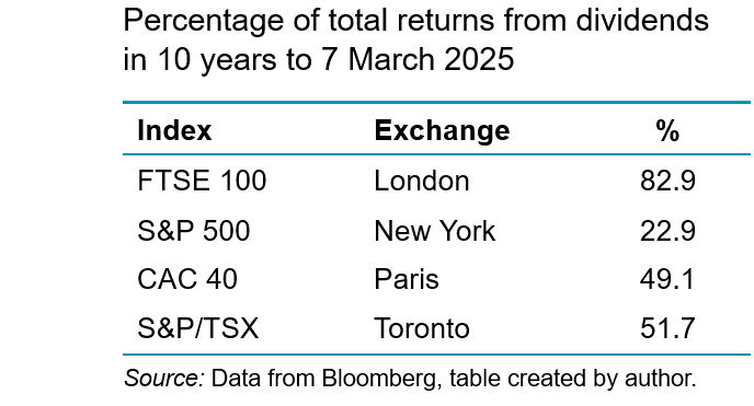
Reinstating this tax benefit could stimulate greater demand for UK equity from this significant sector, boosting liquidity in the London market. Allied to this are proposals from the UK government to consolidate the fragmented UK pension industry to achieve greater scale economies in that channel for investment. This can reduce financing costs, boosting the marginal return from UK investments for these funds, encouraging greater investment in the UK market (ceteris paribus).
Further, the 2.5% stamp duty on share purchases has been viewed as another disincentive for both retail and institutional investors to engage in security trading on the London Stock Exchange. The duty, which is much higher than in peer economies, effectively raises the expected rate of return on UK equites which depresses perceptions of their values and prices. Its removal may raise trading volumes, improving the liquidity of the market and be offset by increased tax revenues in the future. However, the Treasury suggests that the removal of stamp duty is doubtful, since it would create a significant hole in the UK government’s budget.
 Ultimately, many of these reforms may have limited impact on investment. Efforts to boost confidence in the stock market will depend on improving the overall economic environment in the UK. Therefore, it will be the wider policies promoting growth in general which will increase the rates of return offered by London-listed firms and be more significant to attracting capital to London.
However, many of these are controversial themselves, such as relaxing laws around planning permissions and addressing business uncertainties around post-Brexit trading arrangements with the European Union. These broader economic measures could help make the UK generally, and the LSE specifically, more appealing to both domestic and international investors.
Conclusion
The UK government’s proposal to reduce the Cash ISA allowance is part of a broader strategy to boost investment in the stock market and stimulate economic growth. While this change could lead to more capital being directed towards productive investments, it also poses challenges for savers who like the security and simplicity of Cash ISAs.
The ultimate impact will depend on how savers respond to these changes. The potential reduction in overall savings rates could counteract some of the intended benefits. Further, the extent to which they are prepared to channel their savings into UK-listed companies will be important. If many seek higher returns elsewhere, the impact on the UK stock market may be limited. In any case, policies to address the problems of the UK stock market will only work if the wider issues associated with UK productivity and growth are addressed.
Articles
Data
Questions
- Explain how banks use cash ISAs to finance investment through credit creation.
- What do stock markets offer which may boost investment and economic growth?
- What are the issues with the London Stock Exchange which is making it unattractive for raising finance?
- How is the rumoured ISA reform intended to help address these issues?
- Analyse the extent to which it will do so.
- How might some of the broader reforms proposed by the UK government influence rate of return on UK equities and attract capital?
 Economic growth is closely linked to investment. In the short term, there is a demand-side effect: higher investment, by increasing aggregate demand, creates a multiplier effect. GDP rises and unemployment falls. Over the longer term, higher net investment causes a supply-side effect: industrial capacity and potential output rise. This will be from both the greater quantity of capital and, if new investment incorporates superior technology, from a greater productivity of capital.
One of the biggest determinants of investment is certainty about the future: certainty allows businesses to plan investment. Uncertainty, by contrast, is likely to dampen investment. Investment is for future output and if the future is unknown, why undertake costly investment? After all, the cost of investment is generally recouped over several months or year, not immediately. Uncertainty thus increases the risks of investment.
 There is currently great uncertainty in the USA and its trading partners. The frequent changes in policy by President Trump are causing a fall in confidence and consequently a fall in investment. The past few weeks have seen large cuts in US government expenditure as his administration seeks to dismantle the current structure of government. The businesses supplying federal agencies thus face great uncertainty about future contracts. Laid-off workers will be forced to cut their spending, which will have knock-on effect on business, who will cut employment and investment as the multiplier and accelerator work through.
There are also worries that the economic chaos caused by President Trump’s frequent policy changes will cause inflation to rise. Higher inflation will prompt the Federal Reserve to raise interest rates. This, in turn, will increase the cost of borrowing for investment.
Tariff uncertainty
 Perhaps the biggest uncertainty for business concerns the imposition of tariffs. Many US businesses rely on imports of raw materials, components, equipment, etc. Imposing tariffs on imports raises business costs. But this will vary from firm to firm, depending on the proportion of their inputs that are imported. And even when the inputs are from other US companies, those companies may rely on imports and thus be forced to raise prices to their customers. And if, in retaliation, other countries impose tariffs on US goods, this will affect US exporters and discourage them from investing.
For many multinational companies, whether based in the USA or elsewhere, supply chains involve many countries. New tariffs will force them to rethink which suppliers to use and where to locate production. The resulting uncertainty can cause them to delay or cancel investments.
Uncertainty has also been caused by the frequent changes in the planned level of tariffs. With the Trump administration using tariffs as a threat to get trading partners to change policy, the threatened tariff rates have varied depending on how trading partners have responded. There has also been uncertainty on just how the tariff policy will be implemented, making it more difficult for businesses to estimate the effect on them.
Then there are serious issues for the longer term. Other countries will be less willing to sign trade deals with the USA if they will not be honoured. Countries may increasingly look to diverting trade from the USA to other countries.
Video
Articles
- Trump’s erratic trade policies are baffling businesses, threatening investment and economic growth
Associated Press, Paul Wiseman, Anne D’innocenzio and Mae Anderson (6/3/25)
- The world is beginning to tire of Trump’s whiplash leadership
CNN, Stephen Collinson (6/3/25)
- US stocks slide and Nasdaq enters correction as chaos over Trump’s tariffs intensifies
CNN, John Towfighi (6/3/25)
- Trump’s Tariffs And Trade: Uncertainty, Chaos Or Brilliance?
Forbes, Mike Patton (6/3/25)
- How Trump’s second term might affect the market and your finances
The Conversation, Art Durnev (4/3/25)
- US corporate bond investors cautiously navigate trade war uncertainty
Reuters, Matt Tracy (6/3/25)
 This week in Trumponomics: Playing chicken with markets
Yahoo Finance, Rick Newman (8/3/25)
- Measuring fear: What the VIX reveals about market uncertainty
The FRED Blog, Aakash Kalyani (13/2/25)
- Trump shrugs off stock market slump, but economic warning signs loom
The Conversation, Conor O’Kane (17/3/25)
Data
Questions
- Find out what tariffs have been proposed, imposed and changed since Donald Trump came to office on 20 January 2025.
- In what scenario might US investment be stimulated by Donald Trump’s policies?
- What countries’ economies have gained or are set to gain from Donald Trump’s policies?
- What is the USMCA agreement? Do Donald Trump’s policies break this agreement?
- Find out and explain what has happened to the US stock market since January 2025. How do share prices affect business investment?
- Which sector’s shares have risen and which have fallen?
- Using the Data link above, find out what has been happening to the US Policy Uncertainty Index since Donald Trump was elected and explain particular spikes in the index. Is this mirrored in the global Policy Uncertainty Index?
- Are changes in the Policy Uncertainty Index mirrored in the World Uncertainty Index (WUI) and the CBOE Volatility Index: VIX?
 The election of Donald Trump saw the market price of bitcoin rise from $67 839 on election day (5 November 2024) to £106 168 on 18 December: a rise of 56%. It was $104 441 the day before inauguration (20 January 2025).
Trump has been a keen supporter of cryptocurrencies. He has stated that he wants the USA to become the world’s ‘crypto capital’. Indeed, he and Melania Trump have launched their own meme coins hosted on the Solana blockchain. Meme coins are tokens, a form of cryptocurrency, inspired by specific individuals, characters, cartoons or artwork.
On 23 January, three days after his inauguration, President Trump signed an Executive Order. This states that it is:
…the policy of my Administration to support the responsible growth and use of digital assets, blockchain technology, and related technologies across all sectors of the economy, including by … protecting and promoting the ability of individual citizens and private-sector entities alike to access and use for lawful purposes open public blockchain networks without persecution, including the ability to develop and deploy software, to participate in mining and validating, to transact with other persons without unlawful censorship, and to maintain self-custody of digital assets…
The full Executive Order can be read here.
Cryptocurrencies
Although cryptocurrencies can be used for certain transactions and avoid the need for banks, their use as a medium of exchange or unit of account is limited by their price volatility. The supply of national or regional currencies, such as the US dollar, the euro and the pound sterling is controlled by central banks, and central banks have a key mandate of achieving price stability, where price is in terms of their currency’s consumer price index. Although exchange rates fluctuate and thereby affect the prices of internationally traded goods and assets, such fluctuations are small in comparison with crypto price fluctuations.
 The supply of many cryptocurrencies is not controlled with the objective of achieving price stability. Indeed, certain cryptocurrencies, such as bitcoin (the coins with the highest total market value of approximately $2060bn) have a limited maximum supply. The supply of bitcoin in January 2025 is officially 19.81m, 94.3% of the eventual official total of 21m. However, with some 1.8m coins lost, the current effective total supply is more like 18m and the ceiling 19.2m. New coins are created by ‘mining’, involving massive computer power to perform complex calculations. Coins in circulation at any one time are therefore fixed and increase only slowly and at a decelerating rate over time, with increased mining costs per coin. On any one day, however, the supply offered for sale can fluctuate wildly.
Some other crypto currencies also have a long-term supply ceiling and are created by mining. Others, such as ether (the coins with the second highest market value of approximately $394bn) do not have a fixed supply ceiling. They are not created by mining, but by a system known as ‘Proof-of-Stake (PoS)’. This uses the cryptocurrency’s owners, who stake some of their currency, to validate transactions on the Ethereum blockchain. They receive new ether as a reward. PoS uses considerably less energy than mining and hence is regarded as greener.
Unlike mined coins, Ethereum coins (ether) created by PoS can be ‘burned’: i.e. removed from circulating supply. This can more than offset new coins created and lead to a net decrease in supply. See the Fidelity Digital Assets and Paxful links below for a discussion of what determines the net burn/net creation rate of ether. Other coins, such as BNB (Binance’s cryptocurrency), have regular burns to control supply.
 There are some cryptocurrencies that are suitable as a medium of exchange and as a unit of value. These are ‘stablecoins’, whose value is linked 1:1 to a major currency, such as the US dollar or euro. Supply is adjusted to maintain this value. Stablecoins are used primarily for transactions. They account for some two-thirds of all transactions using crypto. They are particularly used for transactions in parts of the world with monetary instability and/or limited access to major currencies.
With the exception of stablecoins, crypto currencies are best seen as assets, rather than as a means of exchange or unit of account. As such, they are more comparable to gold than to conventional currencies.
The market for crypto in the long term
The market price of cryptocurrencies is determined by supply and demand. With limited supply, their price is likely to increase as demand is forecast to increase relative to supply. This is particularly the case with mined cryptocurrencies where there is a ceiling to supply. But even with PoS-created currencies, the amount supplied is likely to increase more slowly than demand, especially with burn mechanisms in place.
With many countries recognising and embracing cryptocurrencies as an asset, so the long-term price should rise. The endorsement by Donald Trump is likely to hasten this process.
The market for crypto in the short term
While the total supply of cryptocurrency is limited, the supply to market can fluctuate wildly, as can demand. This can cause huge gyrations in price.
Short-run demand and supply decisions are governed largely by expectations of future price changes, over anything from the next few hours to the coming months. If people think the price will rise, people will demand more, while those already holding crypto and thinking of selling will hold back. These actions will amplify the very effect they had predicted, namely a rise in price.
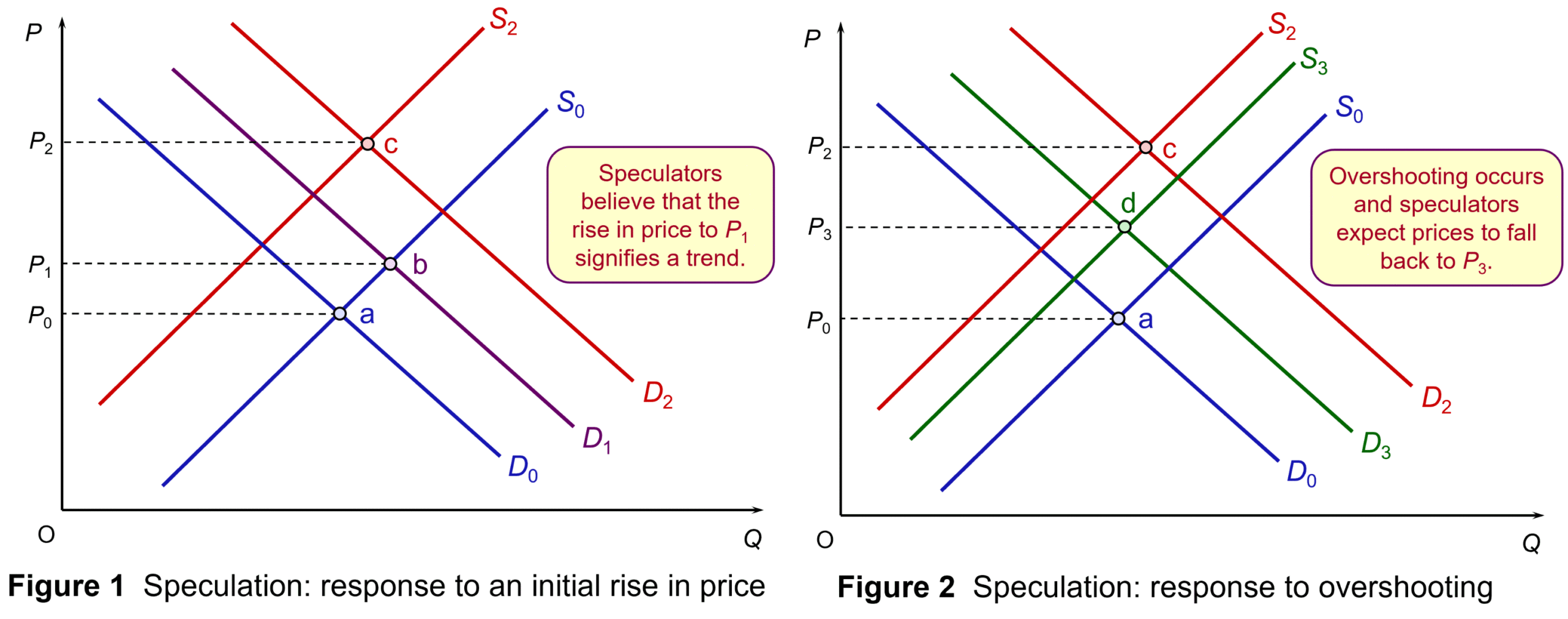
This is illustrated in Figure 1. Assume an initial rise in demand for a particular cryptocurrency from D0 to D1. Equilibrium moves from point a to point b and the price of the cryptocurrency rises from P0 to P1. Speculators believe that this is a trend and that prices will rise further. Demand increases to D2 as purchasers rush to buy; and supply falls to S2 as potential sellers of the crypto hold back. Equilibrium moves to point c and price rises to P2.
But in their exuberance, people may have pushed the price above the level that reflects underlying demand and supply. People respond to this overshooting by selling some of the currency to take advantage of what they see as a temporary high price. In Figure 2, supply rises from S2 to S3. Meanwhile, potential purchasers wait until price has settled back somewhat. Demand falls from D2 to D3. Equilibrium moves to point d, with price falling to P3. (Click here for a PowerPoint of the two diagrams.)

A similar process of speculation takes place when people expect prices to fall, with price potentially plummeting before it then recovers somewhat.
With computer algorithms interpreting underlying economic/political data, the price changes are likely to be frequent, with speculation amplifying these changes.
Articles
- Trump orders crypto working group to draft new regulations, explore national stockpile
Reuters, Hannah Lang and Trevor Hunnicutt (24/1/25)
- Bitcoin soars past $109,000 ahead of possible early action on crypto by Trump
MSN, Alan Suderman (20/1/25)
- 3 Things to Watch as Trump Becomes Memecoin Billionaire and US President
PYMNTS (20/1/25)
- Crypto Community Reacts to Trump and Melania Meme Coins as Market Sinks
Decrypt, Vismaya V (20/1/25)
- Trump’s plan for a strategic bitcoin reserve could trigger a crypto ‘arms race’ and reshape the global economic order
The Conversation, Huw Macartney, Erin McCracken and Robert Elliott (14/1/25)
- Bitcoin’s resurgence: A regulatory reset and a path to innovation
crypto.news, editorial (17/1/25)
- Bitcoin Retreats As Traders Await Trump Crypto Executive Order
Bloomberg on NDTV Profit (21/1/25)
- Bitcoin edges higher as investors shake off initial Trump Day One disappointment
Reuters, Tom Westbrook and Elizabeth Howcroft (21/1/25)
- Has bitcoin’s limited supply driven its rally? Experts weigh in
ABC News, Max Zahn (10/12/24)
Background information
Data
Questions
- What determines the supply of cryptocurrencies (a) in circulation; (b) to the market at any given time?
- Why are the prices of digital currencies so volatile?
- Why or why not are cryptocurrencies a good asset to hold?
- How may speculation (a) amplify and (b) dampen price fluctuations?
- What determines the net burn/net creation rate of ether?
- Should cryptocurrencies be classified as ‘money’?
 On the 29 November, the Bank of England published the results of its latest stress test of the UK financial system. Annual stress testing was introduced in the wake of the 2008 financial crisis. It models the ability of the financial system to withstand severe macroeconomic and financial market conditions. Typically, the focus has been on testing the resilience of the banking system.
This year’s was the first system-wide exploratory scenario (SWES). This recognises the growing significance of ‘shadow banking’. Shadow banking involves borrowing and lending involving non-bank financial institutions (NBFIs). Such institutions sit outside the regulatory cordons around banking but have become significant actors in the financial system.
However, this obscure part of the financial system poses systemic risks which are not clearly understood and from time to time require costly interventions. Examples include: problems in liability-driven investments (LDIs) for pension funds in September 2022; the money market liquidity crisis involving hedge funds in March 2020; the collapse of Long-term Capital Management (LTCM) in 1998 following the Russian Federation’s default (LTCM had significant holdings of Russian government bonds – see linked article on LTCM below).
The growing significance of shadow banking means that regulators have become increasingly concerned about the vulnerabilities in the financial system which arise from outside the traditional banking system.
In this blog we will explain stress-testing of the financial system and trace the rise in shadow banking which motivated the recent system-wide exploratory scenario (SWES). We will discuss the findings of the stress test, highlighting the systemic risks of shadow banking. Finally, we will discuss the implications for the regulation and supervision of the financial system.
What is stress testing?
 Stress testing was introduced by the Bank of England after the financial crisis to assess the ability of the financial system to withstand severe economic and market scenarios.
In the run-up to the 2008 financial crisis, the liquidity and capital buffers of many banks had been extremely thin. These were only able to withstand moderate economic shocks and moderate conditions and buckled under the stresses of the crisis.
Regulators argued that the buffers needed to become much more robust and be able to withstand rare but severe economic and market conditions. The stress testing analogy was derived from engineering, where parts are expected to work not just in benign conditions but also in extreme, hostile environments.
Since 2014, the Bank of England has conducted annual stress testing. Stress testing models the impact of adverse economic conditions on banks’ liquidity, profitability and capital. The results are used to set policy for individual banks (microprudential) and for the system as a whole (macroprudential). Stress test results have allowed the Bank to adjust the loss-absorbing capital that banks must hold to reduce their likelihood of failure.
The scope of the testing has expanded over time to incorporate insurers, central counterparties (financial institutions that provide clearing and settlement services between financial traders) and cyber security. The most recent scenario recognised the increasing significance of non-deposit taking financial institutions in channelling credit. Fifty City of London institutions modelled how a period of intense stress would ripple through the shadow banking sector.
The arcane world of shadow banking
 Shadow banking refers to borrowing and lending which occurs outside the banking sector. Traditionally banking involves taking deposits and using these to finance lending.
Shadow banking involves non-deposit taking financial institutions (NBFIs) such as hedge funds, insurance companies, pension funds, private equity funds, as well as some activities of investment banks. These institutions channel funds in different ways from lenders to borrowers. Typically, they use funds from investors to buy securities through financial markets. The emergence and growth of shadow banking has been explained by changing regulation and innovation.
Its first significant period of expansion in the late 1980s was driven by financial innovation. Increased use of ‘disintermediation’ – the replacement of credit channels through banks with ones through markets – meant an increase in the assets invested through NBFIs.
Despite this process playing a major role in the expansion of housing credit in the run-up to the 2008 financial crisis, it was the significant bailouts that banks received that drew the attention of regulators, not the role of shadow banking. This led to more stringent liquidity and capital requirements for banks under the BASEL III international regulations.
This regulatory tightening limited banks’ ability to offer credit, which meant that much of this activity migrated to the shadow banking sector.
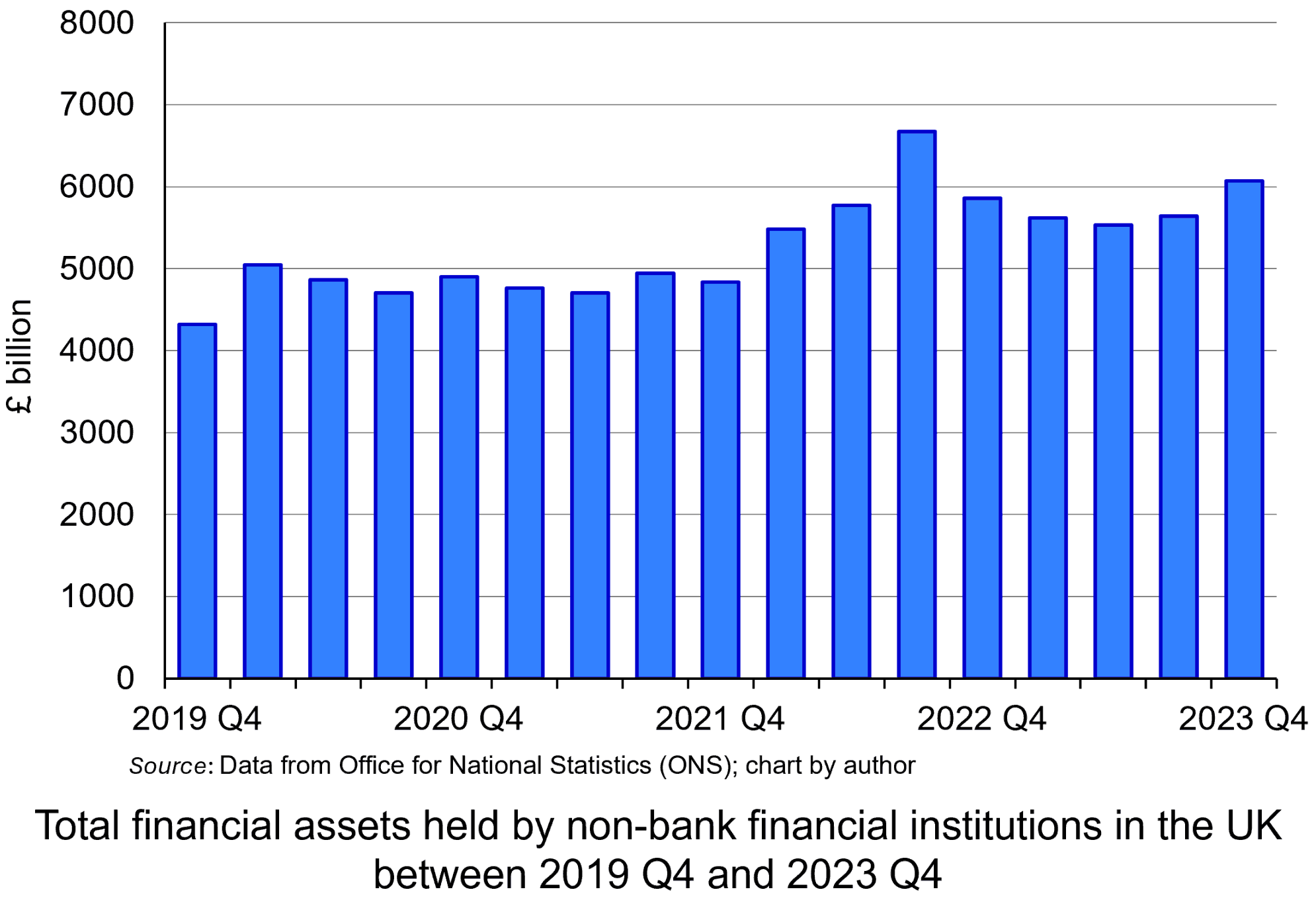 Data from the Bank of England show that the percentage of total assets held by NBFIs rose from 41% in 2007 to 49% in 2020. The chart illustrates the total financial assets held by non-bank financial institutions in the UK between 2019 Q4 and 2023 Q3 (click here for a PowerPoint). The amount held has growth by approximately a third in that time, from £4321bn to £6069bn, peaking at £6670bn in 2022 Q3.
The lack of regulatory oversight stems from the nature of the activities in the shadow banking sector. While NBFIs conduct maturity transformation, provide liquidity and help manage risk, unlike banks, they do not accept deposits and are not part of the payments system involving the general public.
Consequently, the consensus among regulators has been that their activities do not pose the same systemic risks as banking of the breakdown of the payments mechanism and associated collapse in business and consumer confidence. Therefore, NBFIs are not subject to conventional regulation and supervision involving liquidity and capital requirements.
However, as the scale of borrowing and lending running through the sector has grown, this argument has become less difficult to justify. There is a concern that ‘regulatory arbitrage’ is happening and that the systemic risks associated with shadow banking are being underestimated.
The familiar risks of shadow banking
 The systemic consequences of liquidity and solvency problems in the shadow banking sector may not seem obvious. Much of their activities are arcane and technical. However, there are plenty of examples of instances where the problems of hedge funds or pension funds have caused systemic issues.
While the consequences are not the same as those involving banks, in that the payments mechanism is not directly affected, the risks are. Just like banks, these institutions are exposed to liquidity risks, credit default risks and counterparty risks. The concern is that they do not have the same levels of liquidity or capital buffers as banks to insulate them from the consequences of such risks. Therefore, it might not take much economic stress for one or more of these institutions to fail and, given the increasing significance and interconnectedness of these activities, impose significant costs on the rest of the financial system.
It was for this reason that the Bank of England conducted its first system-wide exploratory scenario to analyse the impact of economic and market stress on these institutions and assess the nature and extent of systemic risks which resulted. Fifty City of London institutions modelled how a period of intense stress would ripple through the non-bank sector.
The scenario involved rising geopolitical tensions which caused a sharp rise in risk aversion and a demand for higher expected rates of return as compensation. This produced sharp rises in both sovereign and corporate bond yields and matching sharp declines in asset prices (remember bond yield and prices have a negative relationship).
The scenario found that the position and behaviour of NBFIs amplified the shock. These institutions invest significantly in marketable financial securities and their liquidity and solvency are susceptible to such falling prices.
The sharp decline in asset prices triggered margin calls – payments to cover open loss positions in financial securities. In response to these demands, while some NBFIs’ internal risk and leverage measures were breached, others illustrated greater risk-aversion and took precautionary action. These institutions acted to deleverage, derisk and recapitalise. Given the interconnectedness of financial markets, the individual actions of institutions rippled across financial markets, causing problems in other segments.
The significant decline in asset prices led insurance companies and pension funds to seek to improve their liquidity and solvency position by liquidating positions in money market funds and hedge funds. This, in turn, required these funds to seek liquidity. Such institutions tend to rely a lot on the repo market (involving short-term sale and repurchase credit agreements) to provide liquidity to investors. This avoids them having to sell assets. This practice has echoes of the banking sectors use of the short-term wholesale markets in the run-up to the 2008 financial crisis.
 However, the SWES found that while banks were willing to take on some of the risk, their own concerns about liquidity and counterparty credit risk meant they did not offer sufficient short-term liquidity through the repo markets. If such funding dried up because of a higher risk perception, it could compromise the hedge funds’ ability to raise funds, requiring asset sales. This would amplify the shock to financial markets, driving prices of financial securities even lower.
The scenario concluded that the resulting heavy selling could seize up financial markets, particularly the UK sovereign and corporate bond markets, reducing the ability of companies to finance investment. This is a different type of credit crunch from 2008, which was restricted to banks – but a credit crunch, nonetheless.
At the same time, funds may make capital losses as they sell securities in the downturn. This creates solvency problems and the potential for failure.
In the SWES the institutions were often not able to anticipate how their counterparties, investors, or markets they operate in would behave in the stressed scenario, which echoes the experience of banks in 2007 and 2008 – a significant reason for the ‘crunch’ in banking credit was uncertainty about the creditworthiness of counterparties, meaning that banks were not prepared to lend to anybody.
Conclusion
Since the 2008 financial crisis, there has been a tightening of the regulation and supervision of banks which has limited their ability to channel credit. This has produced an expansion in the shadow banking sector.
However, while the shadow banking sector has not been subject to the same regulation and supervision as banks, there are still potential systemic risks associated with its operations. There have been several examples of such risks in the shadow banking sector which have led regulators to pay more attention. These underpinned the 2024 system-wide exploratory scenario (SWES) conducted by the Bank of England.
The scenario showed the possible transmission mechanism through which problems for NBFIs can have broader consequences. The report nevertheless concluded that:
…the UK financial system was well-capitalised, maintained high levels of liquidity and that asset quality remained strong.
Therefore, the UK financial system was resilient enough to withstand problems in shadow banking.
Although the results of the exercise provide a ‘framework of future system-wide analysis which can be embedded in future market-wide surveillance,’ history indicates that risks tend to exist in obscure and arcane parts of the financial system and that these never tend to be fully appreciated until a crisis occurs. This then tends to involve significant costs for taxpayers.
Articles
- Bank of England warns of risks from non-banks in future markets crisis
Financial Times from MSN, Martin Arnold (29/11/24)
- BoE finds non-bank financial firms pose wider risks in crisis periods
Reuters, Lawrence White (2/12/24)
- Finance Firms Beyond Banks Not Ready For Crisis, BOE Warns
Bloomberg from Yahoo finance, Laura Noonan and Greg Ritchie (29/11/24)
- Shadow Banking System: Definition, Examples, and How It Works
Investopedia, Michael Bromberg (18/10/24)
- US Treasuries: the lessons from March’s market meltdown
Financial Times, Colby Smith and Robin Wigglesworth (29/7/20)
- LDI: the better mousetrap that almost broke the UK
FT Alphaville, Alexandra Scaggs and Louis Ashworth (29/9/22)
- Long-Term Capital Management
CFA Institute, Ron Rimkus (18/4/16)
- Neil Woodford: the continuing fallout of a scandal
Financial Times, Owen Walker (19/3/21)
Bank of England documents and reports
Data
Questions
- Explain stress testing.
- What is shadow banking? Explain the factors driving the growth of credit in this part of the financial system.
- Compare and contrast the liquidity problems of banks with those of non-bank financial institutions (NBFIs).
- Analyse how financial crises can heighten problems of asymmetric information in financial markets.
 In a blog in October 2024, we looked at global uncertainty and how it can be captured in a World Uncertainty Index. The blog stated that ‘We continue to live through incredibly turbulent times. In the past decade or so we have experienced a global financial crisis, a global health emergency, seen the UK’s departure from the European Union, and witnessed increasing levels of geopolitical tension and conflict’.
  The World Uncertainty Index (WUI) tracks uncertainty around the world by applying a form of text mining known as ‘term frequency’ to the country reports produced by the Economist Intelligence Unit (EIU). The words searched for are ‘uncertain’, ‘uncertainty’ and ‘uncertainties’ and the number of times they occur as percentage of the total words is recorded. To produce the WUI this figure is then multiplied by 1m. A higher WUI number indicates a greater level of uncertainty.
 The second chart shows the World Trade Uncertainty Index (WTUI), published on the same site as the WUI (click here for a PowerPoint). The method adopted in its construction therefore mirrors that for the WUI but counts the number of times in EIU country reports ‘uncertainty’ is mentioned within proximity to a word related to trade, such as ‘protectionism’, ‘NAFTA’, ‘tariff’, ‘trade’, ‘UNCTAD’ or ‘WTO.’
 The new Labour government views stimulating higher levels of investment though the London market as an important element in its drive to boost productivity and growth in the UK. Recently, it has been reported that investment institutions have been lobbying the UK government to reduce significantly the tax-free allowance for Cash Individual Savings Accounts (ISAs) as a way to encourage more of UK households’ savings to be channelled through the UK stock market.
 The main reason for the proposed ISA change is to encourage more investment in the UK stock market. By reducing the amount which can be saved in Cash ISAs, the government hopes to encourage savers to invest in Stocks and Shares ISAs instead, particularly ones linked to the UK market. This would increase the amount of finance capital in the market, thereby boosting its liquidity. This would then make it an attractive place for young, vibrant UK and foreign companies to list.
  Further, the desire for a capital injection to finance growth is not the only reason that firms seek stock market listings. Founders of companies may have a lot of wealth invested in the equity of their firms. Selling some of their equity to outside investors through a stock market listing is a way of diversifying their wealth. However, if they are to maximise the potential sale price, there must be an active, liquid secondary market to encourage investors to buy shares in the primary market.
  Demographics may also play a role in this. Many of those who save more are now retired, or near retirement. They are less likely to see the appeal of compounding returns over long periods through investment in shares. Instead, with shorter investment horizons, they may only see the potential for losses associated with Stocks and Shares ISAs. Indeed, they will be starting to liquidate their long-term positions to draw income in retirement. Therefore, they may save less.
  The low valuations of LSE-listed companies compared to their international counterparts, particularly those in the USA, has discouraged growing firms from listing in London. To address this, there have been calls to enhance corporate governance standards and reduce regulatory burdens for listed companies.
 Ultimately, many of these reforms may have limited impact on investment. Efforts to boost confidence in the stock market will depend on improving the overall economic environment in the UK. Therefore, it will be the wider policies promoting growth in general which will increase the rates of return offered by London-listed firms and be more significant to attracting capital to London.
  There is currently great uncertainty in the USA and its trading partners. The frequent changes in policy by President Trump are causing a fall in confidence and consequently a fall in investment. The past few weeks have seen large cuts in US government expenditure as his administration seeks to dismantle the current structure of government. The businesses supplying federal agencies thus face great uncertainty about future contracts. Laid-off workers will be forced to cut their spending, which will have knock-on effect on business, who will cut employment and investment as the multiplier and accelerator work through.
 Perhaps the biggest uncertainty for business concerns the imposition of tariffs. Many US businesses rely on imports of raw materials, components, equipment, etc. Imposing tariffs on imports raises business costs. But this will vary from firm to firm, depending on the proportion of their inputs that are imported. And even when the inputs are from other US companies, those companies may rely on imports and thus be forced to raise prices to their customers. And if, in retaliation, other countries impose tariffs on US goods, this will affect US exporters and discourage them from investing.
 The election of Donald Trump saw the market price of bitcoin rise from $67 839 on election day (5 November 2024) to £106 168 on 18 December: a rise of 56%. It was $104 441 the day before inauguration (20 January 2025).
 The supply of many cryptocurrencies is not controlled with the objective of achieving price stability. Indeed, certain cryptocurrencies, such as bitcoin (the coins with the highest total market value of approximately $2060bn) have a limited maximum supply. The supply of bitcoin in January 2025 is officially 19.81m, 94.3% of the eventual official total of 21m. However, with some 1.8m coins lost, the current effective total supply is more like 18m and the ceiling 19.2m. New coins are created by ‘mining’, involving massive computer power to perform complex calculations. Coins in circulation at any one time are therefore fixed and increase only slowly and at a decelerating rate over time, with increased mining costs per coin. On any one day, however, the supply offered for sale can fluctuate wildly.
 There are some cryptocurrencies that are suitable as a medium of exchange and as a unit of value. These are ‘stablecoins’, whose value is linked 1:1 to a major currency, such as the US dollar or euro. Supply is adjusted to maintain this value. Stablecoins are used primarily for transactions. They account for some two-thirds of all transactions using crypto. They are particularly used for transactions in parts of the world with monetary instability and/or limited access to major currencies.

 On the 29 November, the Bank of England published the results of its latest stress test of the UK financial system. Annual stress testing was introduced in the wake of the 2008 financial crisis. It models the ability of the financial system to withstand severe macroeconomic and financial market conditions. Typically, the focus has been on testing the resilience of the banking system.
 Stress testing was introduced by the Bank of England after the financial crisis to assess the ability of the financial system to withstand severe economic and market scenarios.
 Shadow banking refers to borrowing and lending which occurs outside the banking sector. Traditionally banking involves taking deposits and using these to finance lending.
 Data from the Bank of England show that the percentage of total assets held by NBFIs rose from 41% in 2007 to 49% in 2020. The chart illustrates the total financial assets held by non-bank financial institutions in the UK between 2019 Q4 and 2023 Q3 (click
  However, the SWES found that while banks were willing to take on some of the risk, their own concerns about liquidity and counterparty credit risk meant they did not offer sufficient short-term liquidity through the repo markets. If such funding dried up because of a higher risk perception, it could compromise the hedge funds’ ability to raise funds, requiring asset sales. This would amplify the shock to financial markets, driving prices of financial securities even lower.