 In this blog we show how we can apply fiscal metrics to assess the UK government’s fiscal stance. This captures the extent to which fiscal policy contributes to the level of economic activity in the economy.
Changes in the fiscal stance can then be used to estimate the extent to which discretionary fiscal policy measures represent a tightening or loosening of policy. We can measure the size and direction of fiscal impulses arising from changes in the government’s budgetary position.
Such an analysis is timely given the Autumn Budget presented by Rachel Reeves on 30 October 2024. This was the first Labour budget in 14 years and the first ever to be presented by a female Chancellor of the Exchequer.
We conclude by considering the forecast profile of expenditures and revenues for the next few years and the new fiscal rules announced by the Chancellor.
The fiscal stance
At its most simple, the fiscal stance measures the extent to which fiscal policy increases or decreases demand, thereby influencing growth and inflation (see Box 1.F, page 28, Autumn Budget 2024: see link below).
 The fiscal stance is commonly estimated by measures of pubic-sector borrowing. To understand this, we can refer to the circular flow of income model. In this model, excesses of government spending (an injection) over taxation receipts (a withdrawal or leakage) represent a net injection into the circular flow and hence positively affect the level of aggregate demand for national output, all other things being equal.
A commonly used measure of borrowing in assessing the fiscal stance of the is the primary deficit. Unlike public-sector net borrowing, which is simply the excess of the sector’s spending over its receipts (largely taxation), the primary deficit subtracts net interest costs. It therefore excludes the interest payments on outstanding public-sector debts (and interest income earned on financial assets). The primary deficit can therefore be written as public-sector borrowing less net interest payments.
As discussed in our blog Fiscal impulses in November 2023, the primary deficit captures whether the public sector is able to afford its present fiscal choices by abstracting from debt-serving costs that reflect past fiscal choices. In this way, the primary deficit is a preferable measure to net borrowing both in assessing the impact on economic activity, i.e. the fiscal stance, and in assessing whether today’s fiscal choices will require government to issue additional debt.
 Chart 1 shows public-sector net borrowing and the primary balance as shares of GDP for the UK since financial year 1975/76 (click here for a PowerPoint). The data are from the latest Public Finances Databank published by the Office for Budget Responsibility, published on the day of the Autumn Budget in October (see Data links below).
Over the period 1975/6 to 2023/24, public-sector net borrowing and the primary deficit had averaged 3.8% and 1.3% of GDP respectively. In the financial year 2023/24, they were 4.5% and 1.5% (they had been as high as 15.1% and 14.1% in 2020/21 as a result of COVID support measures). In 2024/25 net borrowing and the primary deficit are forecast to be 4.5% and 1.6% respectively. By 2027/28, while net borrowing is forecast to be 2.3% of GDP, there is forecast to be a primary surplus of 0.7% of GDP.
The Autumn Budget lays out plans for higher tax revenues to contribute two-thirds of the overall reduction in the primary deficit over the forecast period (up to 2029/30), while spending decisions contribute the remaining third.
The largest tax-raising measure is an increase in the employer rate of National Insurance Contributions (NICs) by 1.2 percentage points to 15% from April 2025. This will be levied on employee wages above a Secondary Threshold of £5000, reduced from £9100, which will increase in line with CPI inflation each year from April 2028. (See John’s blog, Raising the minimum wage: its effects on poverty and employment, for an analysis on the effects of this change.) This measure, allowing for other changes to the operation of employer NICs, is expected to raise £122 billion over the forecast period. This amounts to over two-thirds of the additional tax take from the taxation measures taken in the Budget.
 Chart 2 shows both net borrowing and the primary deficit after being cyclically-adjusted (click here for a PowerPoint). This process adjusts these fiscal indicators to account for those parts of spending and taxation that are affected by the position of the economy in the business cycle. These are those parts that act as automatic stabilisers helping, as the name suggests, to stabilise the economy.
The process of cyclical adjustment leads to estimates of receipts and expenditures as if the economy were operating at its potential output level and hence with no output gap. The act of cyclically adjusting the primary deficit, which is our preferred measure of the fiscal stance, allows us to assess better the public sector’s fiscal stance.
Over the period from 1975/6 up to and including 2023/24, the cyclically-adjusted primary deficit (CAPD) averaged 1.1% of GDP. In 2024/25 the CAPD is forecast to be 1.5% of GDP. It then moves to a surplus of 0.5% by 2027/28. It therefore mirrors the path of the unadjusted primary deficit.
Measuring the fiscal impulse
To assess even more clearly the extent to which the fiscal stance is changing, we can use the cyclically-adjusted primary deficit to measure a fiscal impulse. This captures the magnitude of change in discretionary fiscal policy.
The term should not be confused with fiscal multipliers which measure the impact of fiscal changes on outcomes, such as real GDP and employment. Instead, we are interested in the size of the impulse that the economy is being subject to. Specifically, we are measuring discretionary fiscal policy changes that result in structural changes in the government budget and which, therefore, allow an assessment of how much, if at all, a country’s fiscal stance has tightened or loosened.
The size of the fiscal impulse is measured by the year-on-year percentage point change in the cyclically-adjusted public-sector primary deficit (CAPD) as a percentage of GDP. A larger deficit or a smaller surplus indicates a fiscal loosening. This is consistent with a positive fiscal impulse. On the other hand, a smaller deficit or a larger surplus indicates a fiscal tightening. This is consistent with a negative fiscal impulse.
 Chart 3 shows the magnitude of UK fiscal impulses since the mid-1970s (Click here for a PowerPoint file). The scale of the fiscal interventions in response to the COVID-19 pandemic, which included the COVID-19 Business Interruption Loan Scheme (CBILS) and Job Retention Scheme (‘furlough’), stand out sharply. In 2020 the CAPD to output ratio rose from 1.7 to 14.4%. This represents a positive fiscal impulse of 12.4% of GDP.
This was followed in 2021 by a tightening of the fiscal stance, with a negative fiscal impulse of 10.1% of GDP as the CAPD to output fell back to 4.0%. Subsequent tightening was tempered by policy measures to limit the impact on the private sector of the cost-of-living crisis, including the Energy Price Guarantee and Energy Bills Support Scheme.
For comparison, the fiscal response to the global financial crisis from 2007 to 2009 saw a cumulative positive fiscal impulse of 5.6% of GDP. While smaller in comparison to the discretionary fiscal responses to the COVID-19 pandemic, it nonetheless represented a sizeable loosening of the fiscal stance.
 Chart 4 focuses on the implied fiscal impulse for the forecast period up to 2029/30 (click here for a PowerPoint). The period is notable for a negative fiscal impulse each year. Across the period as a whole, this there is a cumulative negative fiscal impulse of 2.6% of GDP. Most of the ‘heavy-lifting’ of the fiscal consolidation occurs in the three financial years from 2025/26 during which there is a cumulative negative impulse of 2.0% of GDP.
Looking forward
To conclude, we consider the implications for the projected profiles of public-sector spending, receipts and liabilities over the forecast period up to 2029/30.
 Chart 5 plots data since the mid-1950s (click here for a PowerPoint). It shows the size of total public-sector spending (also known as ‘total managed expenditures’), taxation receipts (sometimes referred as the ‘tax burden’) and total public-sector receipts as shares of GDP. This last one includes additional receipts, such as interest payments on financial assets and income generated by public corporations, as well as taxation receipts.
The OBR forecasts that in real terms (i.e. after adjustment for inflation), public-sector spending will increase on average over the period from 2025/26 to 2029/30 by 1.4% per year, but with total receipts due to rise more quickly at 2.5% per year and taxation receipts by 2.8% per year. The implications of this, as discussed in the OBR’s October 1014 Economic and Fiscal Outlook (see link below), are that:
the size of the state is forecast to settle at 44% of GDP by the end of the decade, almost 5 percentage points higher than before the pandemic” while additional tax revenues will “push the tax take to a historic high of 38% of GDP by 2029-30
Finally, the government has committed to two key rules: a stability rule and an investment rule.
The stability rule. This states that the current budget must be in surplus by 2029/30 or, once 2029/30 becomes the third year of the forecast period, it will be in balance or surplus every third year of the rolling forecast period thereafter. The current budget refers to the difference between receipts and expenditures other than capital expenditures. In effect, it captures the ability of government to meet day-to-day spending and is intended to ensure that over the medium term any borrowing is solely for investment. It is important to note that ‘balance’ is defined in a range of between a deficit and surplus of no more than 0.5% of GDP.
The stability rule replaces the borrowing rule of the previous government that public net borrowing, therefore inclusive of investment expenditures, was not to exceed 3% of GDP by the fifth year of the rolling forecast period.
 The investment rule. The government is planning to increase investment. In order to do this in a financially sustainable way, the investment rule states that public-sector net financial liabilities (PSNFL) or net financial debt for short, is falling as a share GDP by 2029/30, until 2029/30 becomes the third year of the forecast period. PSNFL should then fall by the third year of the rolling forecast period. PSNFL is a broader measure of the sector’s balance sheet than public-sector net debt (PSND), which was targeted under the previous government and which was required to fall by the fifth year of the rolling forecast period.
The new target, as well as now extending to the Bank of England, ‘nets off’ not just liquid assets (i.e. cash in the bank and foreign exchange reserves) but also financial assets such as shares and money owed to it, including expected student loan repayments. While liabilities are broader too, including for example, the local government pension scheme, the impact is expected to reduce the new liabilities target by £236 billion or 8.2 percentage points of GDP in 2024/25. The hope is that both rules can support what the Budget Report labels a ‘step change in investment’.
 As Chart 6 shows, public investment as a share of GDP has not exceeded 6% this century and during the 2010s averaged only 4.4% (click here for a PowerPoint). The forecast has it rising above 5% for a time, but easing to 4.8% by end of the period.
This suggests more progress will be needed if the UK is to experience a significant and enduring increase in public investment. Of course, this needs to be set in the context of the wider public finances and is illustrative of the choices facing fiscal policymakers across the globe after the often violent shocks that have rocked economies and impacted on the state of the public finances in recent years.
Articles
Official documents
Data
Questions
- Explain what is meant by the following fiscal terms:
(a) Structural deficit,
(b) Automatic stabilisers,
(c) Discretionary fiscal policy,
(d) Public-sector net borrowing,
(e) Primary deficit,
(f) Current budget balance,
(g) Public-sector net financial liabilities (PSNFL).
- Explain the difference between a fiscal impulse and a fiscal multiplier.
- In designing fiscal rules what issues might policymakers need to consider?
- What are key differences between the fiscal rules of the previous Conservative government and the new Labour government in the UK? What economic arguments would you make for and against the ‘old’ and ‘new’ fiscal rules?
- What is meant by the ‘sustainability’ of the public finances? What factors might impact on their sustainability?
 The past decade or so has seen large-scale economic turbulence. As we saw in the blog Fiscal impulses, governments have responded with large fiscal interventions. The COVID-19 pandemic, for example, led to a positive fiscal impulse in the UK in 2020, as measured by the change in the structural primary balance, of over 12 per cent of national income.
The scale of these interventions has led to a significant increase in the public-sector debt-to-GDP ratio in many countries. The recent interest rates hikes arising from central banks responding to inflationary pressures have put additional pressure on the financial well-being of governments, not least on the financing of their debt. Here we discuss these pressures in the context of the ‘r – g’ rule of sustainable public debt.
Public-sector debt and borrowing
 Chart 1 shows the path of UK public-sector net debt and net borrowing, as percentages of GDP, since 1990. Debt is a stock concept and is the result of accumulated flows of past borrowing. Net debt is simply gross debt less liquid financial assets, which mainly consist of foreign exchange reserves and cash deposits. Net borrowing is the headline measure of the sector’s deficit and is based on when expenditures and receipts (largely taxation) are recorded rather than when cash is actually paid or received. (Click here for a PowerPoint of Chart 1)
Chart 1 shows the impact of the fiscal interventions associated with the global financial crisis and the COVID-19 pandemic, when net borrowing rose to 10 per cent and 15 per cent of GDP respectively. The former contributed to the debt-to-GDP ratio rising from 35.6 per cent in 2007/8 to 81.6 per cent in 2014/15, while the pandemic and subsequent cost-of-living interventions contributed to the ratio rising from 85.2 per cent in 2019/20 to around 98 per cent in 2023/24.
Sustainability of the public finances
") The ratcheting up of debt levels affects debt servicing costs and hence the budgetary position of government. Yet the recent increases in interest rates also raise the costs faced by governments in financing future deficits or refinancing existing debts that are due to mature. In addition, a continuation of the low economic growth that has beset the UK economy since the global financial crisis also has implications for the burden imposed on the public sector by its debts, and hence the sustainability of the public finances. After all, low growth has implications for spending commitments, and, of course, the flow of receipts.
The ratcheting up of debt levels affects debt servicing costs and hence the budgetary position of government. Yet the recent increases in interest rates also raise the costs faced by governments in financing future deficits or refinancing existing debts that are due to mature. In addition, a continuation of the low economic growth that has beset the UK economy since the global financial crisis also has implications for the burden imposed on the public sector by its debts, and hence the sustainability of the public finances. After all, low growth has implications for spending commitments, and, of course, the flow of receipts.
The analysis therefore implies that the sustainability of public-sector debt is dependent on at least three factors: existing debt levels, the implied average interest rate facing the public sector on its debts, and the rate of economic growth. These three factors turn out to underpin a well-known rule relating to the fiscal arithmetic of public-sector debt. The rule is sometimes known as the ‘r – g’ rule (i.e. the interest rate minus the growth rate).
Underpinning the fiscal arithmetic that determines the path of public-sector debt is the concept of the ‘primary balance’. This is the difference between the sector’s receipts and its expenditures less its debt interest payments. A primary surplus (a positive primary balance) means that receipts exceed expenditures less debt interest payments, whereas a primary deficit (a negative primary balance) means that receipts fall short. The fiscal arithmetic necessary to prevent the debt-to-GDP ratio rising produces the following stable debt equation or ‘r – g’ rule:
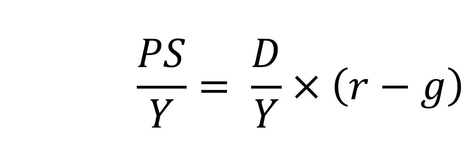
On the left-hand side of the stable debt equation is the required primary surplus (PS) to GDP (Y) ratio. Moving to the right-hand side, the first term is the existing debt-to-GDP ratio (D/Y). The second term ‘r – g’, is the differential between the average implied interest rate the government pays on its debt and the growth rate of the economy. These terms can be expressed in either nominal or real terms as this does not affect the differential.
To illustrate the rule consider a country whose existing debt-to-GDP ratio is 1 (i.e. 100 per cent) and the ‘r – g’ differential is 0.02 (2 percentage points). In this scenario they would need to run a primary surplus to GDP ratio of 0.02 (i.e. 2 percent of GDP).
The ‘r – g‘ differential
The ‘r – g’ differential reflects macroeconomic and financial conditions. The fiscal arithmetic shows that these are important for the dynamics of public-sector debt. The fiscal arithmetic is straightforward when r = g as any primary deficit will cause the debt-to-GDP ratio to rise, while a primary surplus will cause the ratio to fall. The larger is g relative to r the more favourable are the conditions for the path of debt. Importantly, if the differential is negative (r < g), it is possible for the public sector to run a primary deficit, up to the amount that the stable debt equation permits.
 Consider Charts 2 and 3 to understand how the ‘r – g’ differential has affected debt sustainability in the UK since 1990. Chart 2 plots the implied yield on 10-year government bonds, alongside the annual rate of nominal growth (click here for a PowerPoint). As John explains in his blog The bond roller coaster, the yield is calculated as the coupon rate that would have to be paid for the market price of a bond to equal its face value. Over the period, the average annual nominal growth rate was 4.5 per cent, while the implied interest rate was almost identical at 4.6 per cent. The average annual rate of CPI inflation over this period was 2.8 per cent.
 Chart 3 plots the ‘r – g’ differential which is simply the difference between the two series in Chart 2, along with a 12-month rolling average of the differential to help show better the direction of the differential by smoothing out some of the short-term volatility (click here for a PowerPoint). The differential across the period is a mere 0.1 percentage points implying that macroeconomic and financial conditions have typically been neutral in supporting debt sustainability. However, this does mask some significant changes across the period.
We observe a general downward trend in the ‘r – g’ differential from 1990 up to the time of the global financial crisis. Indeed between 2003 and 2007 we observe a favourable negative differential which helps to support the sustainability of public debt and therefore the well-being of the public finances. This downward trend of the ‘r – g’ differential was interrupted by the financial crisis, driven by a significant contraction in economic activity. This led to a positive spike in the differential of over 7 percentage points.
 Yet the negative differential resumed in 2010 and continued up to the pandemic. Again, this is indicative of the macroeconomic and financial environments being supportive of the public finances. It was, however, largely driven by low interest rates rather than by economic growth.
Consequently, the negative ‘r – g’ differential meant that the public sector could continue to run primary deficits during the 2010s, despite the now much higher debt-to-GDP ratio. Yet, weak growth was placing limits on this. Chart 4 indeed shows that primary deficits fell across the decade (click here for a PowerPoint).
The pandemic and beyond
 The pandemic saw the ‘r – g’ differential again turn markedly positive, averaging 7 percentage points in the four quarters from Q2 of 2020. While the differential again turned negative, the debt-to-GDP ratio had also increased substantially because of large-scale fiscal interventions. This made the negative differential even more important for the sustainability of the public finances. The question is how long the negative differential can last.
Looking forward, the fiscal arithmetic is indeed uncertain and worryingly is likely to be less favourable. Interest rates have risen and, although inflationary pressures may be easing somewhat, interest rates are likely to remain much higher than during the past decade. Geopolitical tensions and global fragmentation pose future inflationary concerns and a further drag on growth.
As well as the short-term concerns over growth, there remain long-standing issues of low productivity which must be tackled if the growth of the UK economy’s potential output is to be raised. These concerns all point to the important ‘r – g’ differential become increasingly less negative, if not positive. If so the fiscal arithmetic could mean increasingly hard maths for policymakers.
Articles
- The budget deficit: a short guide
House of Commons Library (8/6/23)
- If markets are right about long real rates, public debt ratios will increase for some time. We must make sure that they do not explode.
Peterson Institute for International Economics, Olivier Blanchard (6/11/23)
- The UK government’s debt nightmare
ITV News, Robert Peston (13/7/23)
- National debt could hit 300% of GDP by 2070s, independent watchdog the OBR warns
Sky News, James Sillars (13/7/23)
- How much money is the UK government borrowing, and does it matter?
BBC News (20/10/23)
- Cost of national debt hits 20-year high
BBC News, Vishala Sri-Pathma & Faisal Islam (4/10/23)
- Bond markets could see ‘mini boom-bust cycles’ as global government debt to soar by $5 trillion a yea
Markets Insider, Filip De Mott (16/11/23)
- The counterintuitive truth about deficits for bond investors
Financial Times, Matt King (17/11/23)
- UK government borrowing almost £20bn lower than expected
The Guardian, Richard Partington (20/10/23)
- Controlling debt is just a means — it is not a government’s end
Financial Times, Martin Wolf (13/11/23)
Data
Questions
- What is meant by each of the following terms: (a) net borrowing; (b) primary deficit; (c) net debt?
- Explain how the following affect the path of the public-sector debt-to-GDP ratio: (a) interest rates; (b) economic growth; (c) the existing debt-to-GDP ratio.
- Which factors during the 2010s were affecting the fiscal arithmetic of public debt positively, and which negatively?
- Discuss the prospects for the fiscal arithmetic of public debt in the coming years.
- Assume that a country has an existing public-sector debt-to-GDP ratio of 60 percent.
(a) Using the ‘rule of thumb’ for public debt dynamics, calculate the approximate primary balance it would need to run in the coming year if the expected average real interest rate on the debt were 3 per cent and real economic growth were 2 per cent?
(b) Repeat (a) but now assume that real economic growth is expected to be 4 per cent.
(c) Repeat (a) but now assume that the existing public-sector debt-to-GDP ratio is 120 per cent.
(d) Using your results from (a) to (c) discuss the factors that affect the fiscal arithmetic of the growth of public-sector debt.
 In his blog, The bond roller coaster, John looks at the pricing of government bonds and details how, in recent times, governments wishing to borrow by issuing new bonds are having to offer higher coupon rates to attract investors. The interest rate hikes by central banks in response to global-wide inflationary pressures have therefore spilt over into bond markets. Though this evidences the ‘pass through’ of central bank interest rate increases to the general structure of interest rates, it does, however, pose significant costs for governments as they seek to finance future budgetary deficits or refinance existing debts coming up to maturity.
The Autumn Statement in the UK is scheduled to be made on 22 November. This, as well as providing an update on the economy and the public finances, is likely to include a number of fiscal proposals. It is thus timely to remind ourselves of the size of recent discretionary fiscal measures and their potential impact on the sustainability of the public finances. In this first of two blogs, we consider the former: the magnitude of recent discretionary fiscal policy changes.
First, it is important to define what we mean by discretionary fiscal policy. It refers to deliberate changes in government spending or taxation. This needs to be distinguished from the concept of automatic stabilisers, which relate to those parts of government budgets that automatically result in an increase (decrease) of spending or a decrease (increase) in tax payments when the economy slows (quickens).
The suitability of discretionary fiscal policy measures depends on the objectives they trying to fulfil. Discretionary measures can be implemented, for example, to affect levels of public-service provision, the distribution of income, levels of aggregate demand or to affect longer-term growth of aggregate supply. As we shall see in this blog, some of the large recent interventions have been conducted primarily to support and stabilise economic activity in the face of heightened economic volatility.
 Discretionary fiscal measures in the UK are usually announced in annual Budget statements in the House of Commons. These are normally in March, but discretionary fiscal changes can be made in the Autumn Statement too. The Autumn Statement of October 2022, for example, took on significant importance as the new Chancellor of the Exchequer, Jeremy Hunt, tried to present a ‘safe pair hands’ following the fallout and market turbulence in response to the fiscal statement by the former Chancellor, Kwasi Kwarteng, on 23 September that year.
The fiscal impulse
The large-scale economic turbulence of recent years associated first with the global financial crisis of 2007–9 and then with the COVID-19 pandemic and the cost-of-living crisis, has seen governments respond with significant discretionary fiscal measures. During the COVID-19 pandemic, examples of fiscal interventions in the UK included the COVID-19 Business Interruption Loan Scheme (CBILS), grants for retail, hospitality and leisure businesses, the COVID-19 Job Retention Scheme (better known as the furlough scheme) and the Self-Employed Income Support Scheme.
 The size of discretionary fiscal interventions can be measured by the fiscal impulse. This captures the magnitude of change in discretionary fiscal policy and thus the size of the stimulus. The concept is not to be confused with fiscal multipliers, which measure the impact of fiscal changes on economic outcomes, such as real national income and employment.
By measuring fiscal impulses, we can analyse the extent to which a country’s fiscal stance has tightened, loosened, or remained unchanged. In other words, we are attempting to capture discretionary fiscal policy changes that result in structural changes in the government budget and, therefore, in structural changes in spending and/or taxation.
To measure structural changes in the public-sector’s budgetary position, we calculate changes in structural budget balances.
A budget balance is simply the difference between receipts (largely taxation) and spending. A budget surplus occurs when receipts are greater than spending, while a deficit (sometimes referred to as net borrowing) occurs if spending is greater than receipts.
A structural budget balance cyclically-adjusts receipts and spending and hence adjusts for the position of the economy in the business cycle. In doing so, it has the effect of adjusting both receipts and spending for the effect of automatic stabilisers. Another way of thinking about this is to ask what the balance between receipts and spending would be if the economy were operating at its potential output. A deterioration in a structural budget balance infers a rise in the structural deficit or fall in the structural surplus. This indicates a loosening of the fiscal stance. An improvement in the structural budget balance, by contrast, indicates a tightening.
The size of UK fiscal impulses
A frequently-used measure of the fiscal impulse involves the change in the cyclically-adjusted public-sector primary deficit.
 A primary deficit captures the extent to which the receipts of the public sector fall short of its spending, excluding its spending on debt interest payments. It essentially captures whether the public sector is able to afford its ‘new’ fiscal choices from its receipts; it excludes debt-servicing costs, which can be thought of as reflecting fiscal choices of the past. By using a cyclically-adjusted primary deficit we are able to isolate more accurately the size of discretionary policy changes. Chart 1 shows the UK’s actual and cyclically-adjusted primary deficit as a share of GDP since 1975, which have averaged 1.3 and 1.1 per cent of GDP respectively. (Click here for a PowerPoint of the chart.)
The size of the fiscal impulse is measured by the year-on-year percentage point change in the cyclically-adjusted public-sector primary deficit as a percentage of GDP. A larger deficit or a smaller surplus indicates a fiscal loosening (a positive fiscal impulse), while a smaller deficit or a larger surplus indicates a fiscal tightening (a negative fiscal impulse).
 Chart 2 shows the magnitude of UK fiscal impulses since 1980. It captures very starkly the extent of the loosening of the fiscal stance in 2020 in response to the COVID-19 pandemic. (Click here for a PowerPoint of the chart.) In 2020 the cyclically-adjusted primary deficit to GDP ratio rose from 1.67 to 14.04 per cent. This represents a positive fiscal impulse of 12.4 per cent of GDP.
A tightening of fiscal policy followed the waning of the pandemic. 2021 saw a negative fiscal impulse of 10.1 per cent of GDP. Subsequent tightening was tempered by policy measures to limit the impact on the private sector of the cost-of-living crisis, including the Energy Price Guarantee and Energy Bills Support Scheme.
In comparison, the fiscal response to the global financial crisis led to a cumulative increase in the cyclically-adjusted primary deficit to GDP ratio from 2007 to 2009 of 5.0 percentage points. Hence, the financial crisis saw a positive fiscal impulse of 5 per cent of GDP. While smaller in comparison to the discretionary fiscal responses to the COVID-19 pandemic, it was, nonetheless, a sizeable loosening of the fiscal stance.
Sustainability and well-being of the public finances
The recent fiscal interventions have implications for the financial well-being of the public-sector. Not least, the financing of the positive fiscal impulses has led to a substantial growth in the accumulated size of the public-sector debt stock. At the end of 2006/7 the public-sector net debt stock was 35 per cent of GDP; at the end of the current financial year, 2023/24, it is expected to be 103 per cent.
As we saw at the outset, in an environment of rising interest rates, the increase in the public-sector debt to GDP ratio creates significant additional costs for government, a situation that is made more difficult for government not only by the current flatlining of economic activity, but by the low underlying rate of economic growth seen since the financial crisis. The combination of higher interest rates and lower economic growth has adverse implications for the sustainability of the public finances and the ability of the public sector to absorb the effects of future economic crises.
Articles
- Autumn Statement 2023: When is it and how will it affect me?
BBC News (16/11/23)
- What is the Autumn Statement?
House of Commons Library (13/11/23)
- Putting the fiscal toothpaste back into the tube: It’s time to normalise the euro area fiscal stance in 2024
VoxEU, Niels Thygesen, Roel Beetsma, Massimo Bordignon, Xavier Debrun, Mateusz Szczurek, Martin Larch, Matthias Busse, Mateja Gabrijelcic, Laszlo Jankovics and Janis Malzubris (30/6/23)
- Euro zone should tighten fiscal policy in 2024 to curb inflation, European Fiscal Board says
Reuters, Jan Strupczewski (28/6/23)
- Hutchins Center Fiscal Impact Measure: Federal, State and Local Fiscal Policy and the Economy
Brookings, Eli Asdourian, Louise Sheiner, and Lorae Stojanovic (27/10/23)
Report
- IFS Green Budget
Institute for Fiscal Studies, Carl Emmerson, Paul Johnson and Ben Zaranko (eds) (October 2023)
Data
Questions
- Explain what is meant by the following fiscal terms: (a) structural deficit; (b) automatic stabilisers; (c) discretionary fiscal policy; (d) primary deficit.
- What is the difference between current and capital public expenditures? Give some examples of each.
- Consider the following two examples of public expenditure: grants from government paid to the private sector for the installation of energy-efficient boilers, and welfare payments to unemployed people. How are these expenditures classified in the public finances and what fiscal objectives do you think they meet?
- Which of the following statements about the primary balance is FALSE?
(a) In the presence of debt interest payments a primary deficit will be smaller than a budget deficit.
(b) In the presence of debt interest payments a primary surplus will be smaller than a budget surplus.
(c) The primary balance differs from the budget balance by the size of debt interest payments.
(d) None of the above.
- Explain the difference between a fiscal impulse and a fiscal multiplier.
- Why is low economic growth likely to affect the sustainability of the public finances? What other factors could also matter?
 On 10 March, the House of Representatives gave final approval to President Biden’s $1.9tr fiscal stimulus plan (the American Rescue Plan). Worth over 9% of GDP, this represents the third stage of an unparalleled boost to the US economy. In March 2020, President Trump secured congressional agreement for a $2.2tr package (the CARES Act). Then in December 2020, a bipartisan COVID relief bill, worth $902bn, was passed by Congress.
By comparison, the Obama package in 2009 in response to the impending recession following the financial crisis was $831bn (5.7% of GDP).
The American Rescue Plan
The Biden stimulus programme consists of a range of measures, the majority of which provide monetary support to individuals. These include a payment of $1400 per person for single people earning less than $75 000 and couples less than $150 000. These come on top of payments of $1200 in March 2020 and $600 in late December. In addition, the top-up to unemployment benefits of $300 per week agreed in December will now continue until September. Also, annual child tax credit will rise from $2000 annually to as much as $3600 and this benefit will be available in advance.
 Other measures include $350bn in grants for local governments depending on their levels of unemployment and other needs; $50bn to improve COVID testing centres and $20bn to develop a national vaccination campaign; $170bn to schools and universities to help them reopen after lockdown; and grants to small businesses and specific grants to hard-hit sectors, such as hospitality, airlines, airports and rail companies.
Despite supporting the two earlier packages, no Republican representative or senator backed this latest package, arguing that it was not sufficiently focused. As a result, reaction to the package has been very much along partisan lines. Nevertheless, it is supported by some 90% of Democrat voters and 50% of Republican voters.
Is the stimulus the right amount?
Although the latest package is worth $1.9tr, aggregate demand will not expand by this amount, which will limit the size of the multiplier effect. The reason is that the benefits multiplier is less than the government expenditure multiplier as some of the extra money people receive will be saved or used to reduce debts.
With $3tr representing some 9% of GDP, this should easily fill the estimated negative output gap of between 2% and 3%, especially when multiplier effects are included. Also, with savings having increased during the recession to put them some 7% above normal, the additional amount saved may be quite small, and wealthier Americans may begin to reduce their savings and spend a larger proportion of their income.
 So the problem might be one of excessive stimulus, which in normal times could result in crowding out by driving up interest rates and dampening investment. However, the Fed is still engaged in a programme of quantitative easing. Between mid-March 2020 and the end of March 2021, the Fed’s portfolio of securities held outright grew from $3.9tr to $7.2tr. What is more, many economists predict that inflation is unlikely to rise other than very slightly. If this is so, it should allow the package to be financed easily. Debt should not rise to unsustainable levels.
Other economists argue, however, that inflationary expectations are rising, reflected in bond yields, and this could drive actual inflation and force the Fed into the awkward dilemma of either raising interest rates, which could have a significant dampening effect, or further increasing money supply, potentially leading to greater inflationary problems in the future.
A lot will depend what happens to potential GDP. Will it rise over the medium term so that additional spending can be accommodated? If the rise in spending encourages an increase in investment, this should increase potential GDP. This will depend on business confidence, which may be boosted by the package or may be dampened by worries about inflation.
Additional packages to come
 Potential GDP should also be boosted by two further packages that Biden plans to put to Congress.
The first is a $2.2tr infrastructure investment plan, known as the American Jobs Plan. This is a 10-year plan to invest public money in transport infrastructure (such as rebuilding 20 000 miles of road and repairing bridges), public transport, electric vehicles, green housing, schools, water supply, green power generation, modernising the power grid, broadband, R&D in fields such as AI, social care, job training and manufacturing. This will be largely funded through tax increases, such as gradually raising corporation tax from 21% to 28% (it had been cut from 35% to 21% by President Trump) and taxing global profits of US multinationals. However, the spending will generally precede the increased revenues and thus will raise aggregate demand in the initial years. Only after 15 years are revenues expected to exceed costs.
The second is a yet-to-be announced plan to increase spending on childcare, healthcare and education. This should be worth at least $1tr. This will probably be funded by tax increases on income, capital gains and property, aimed largely at wealthy individuals. Again, it is hoped that this will boost potential GDP, in this case by increasing labour productivity.
With earlier packages, the total increase in public spending will be over $8tr. This is discretionary fiscal policy writ large.
Articles
- Biden’s $1.9 trillion COVID-19 bill wins final approval in House
Reuters, Susan Cornwell and Makini Brice (10/3/21)
- Biden’s Covid stimulus plan: It costs $1.9tn but what’s in it?
BBC News, Natalie Sherman (6/3/21)
- Biden’s $1.9 Trillion Challenge: End the Coronavirus Crisis Faster
New York Times, Jim Tankersley and Sheryl Gay Stolberg (22/3/21)
- Joe Biden writes a cheque for America – and the rest of the world
The Observer, Phillip Inman (13/3/21)
- Spend or save: Will Biden’s stimulus cheques boost the economy?
Aljazeera, Cinnamon Janzer (9/3/21)
- After Biden stimulus, US economic growth could rival China’s for the first time in decades
CNN, Matt Egan (12/3/21)
- Larry Summers, who called out inflation fears with Biden’s $1.9 trillion COVID-19 relief package, says the US is seeing ‘least responsible’ macroeconomic policy in 40 years
Business Insider, John L. Dorman (21/3/21)
- With $1.9 Trillion in New Spending, America Is Headed for Financial Fragility
Barron’s, Leslie Lipschitz and Josh Felman (30/3/21)
- Biden unveils ‘once-in-a generation’ $2tn infrastructure investment plan
The Guardian, Lauren Gambino (31/3/21)
- Biden unveils $2tn infrastructure plan and big corporate tax rise
Financial Times, James Politi (31/3/21)
- The Observer view on Joe Biden’s audacious spending plans
The Observer, editorial (11/4/21)
Videos
Questions
- Draw a Keynesian cross diagram to show the effect of an increase in benefits when the economy is operating below potential GDP.
- What determines the size of the benefits multiplier?
- Explain what is meant by the output gap. How might the pandemic and accompanying emergency health measures have affected the size of the output gap?
- How are expectations relevant to the effectiveness of the stimulus measures?
- What is likely to determine the proportion of the $1400 stimulus cheques that people spend?
- Distinguish between resource crowding out and financial crowding out. Is the fiscal stimulus package likely to result in either form of crowding out and, if so, what will determine by how much?
- What is the current monetary policy of the Fed? How is it likely to impact on the effectiveness of the fiscal stimulus?
 Rishi Sunak delivered his 2021 UK Budget on 3 March. It illustrates the delicate balancing act that governments in many countries face as the effects of the coronavirus pandemic persist and public-sector debt soars. He announced that he would continue supporting the economy through various forms of government expenditure and tax relief, but also announced tax rises over the medium term to begin addressing the massively increased public-sector debt.
Key measures of support for people and businesses include:
- An extension of the furlough scheme until the end of September, with employees continuing to be paid 80% of their wages for hours they cannot work, but with employers having to contribute 10% in July and 20% in August and September.
- Support for the self-employed also extended until September, with the scheme being widened to make 600 000 more self-employed people eligible.
- The temporary £20 increase to Universal Credit, introduced in April last year and due to end on 31 March this year, to be extended to the end of September.
- Stamp duty holiday on house purchases in England and Northern Ireland, under which there is no tax liability on sales of less than £500 000, extended from the end of March to the end of June.
- An additional £1.65bn to support the UK’s vaccination rollout.
- VAT rate for hospitality firms to be maintained at the reduced 5% rate until the end of September and then raised to 12.5% (rather than 20%) for a further six months.
- A range of grants for the arts, sport, shops , other businesses and apprenticeships.
- Business rates holiday for hospitality firms in England extended from the end of March to the end of June and then with a discount of 66% until April 2022.
- 130% of investment costs can be offset against tax – a new tax ‘super-deduction’.
- No tax rises on alcohol, tobacco or fuel.
- New UK Infrastructure Bank to be set up in Leeds with £12bn in capital to support £40bn worth of public and private projects.
- Increased grants for devolved nations and grants for 45 English towns.
It has surprised many commentators that there was no announcement of greater investment in the NHS or more money for social care beyond the £3bn for the NHS and £1bn for social care announced in the November Spending Review. The NHS England budget will fall from £148bn in 2020/21 to £139bn in 2021/22.
Effects on borrowing and GDP

The net effect of these measures for the two financial years 2020 to 2022 is forecast by the Treasury to be an additional £37.5bn of government expenditure and a £27.3bn reduction in tax revenue (see Table 2.1 in Budget 2021). This takes the total support since the start of the pandemic to £352bn across the two years.
According to the OBR, this will result in public-sector borrowing being 16.9% of GDP in 2020/21 (the highest since the Second World War) and 10.3% of GDP in 2021/22. Public-sector debt will be 107.4% of GDP in 2021/22, rising to 109.7% in 2023/24 and then falling to 103.8% in 2025/26.
 Faced with this big increase in borrowing, the Chancellor also announced some measures to raise tax revenue beginning in two years’ time when, hopefully, the economy will have grown. Indeed, the OBR forecasts that GDP will grow by 4.0% in 2021 and 7.3% in 2022, with the growth rate then settling at around 1.7% from 2023 onwards. He announced that:
- Corporation tax on company profits over £250 000 will rise from 19% to 25% in April 2023. Rates for profits under £50 000 will remain at the current rate of 19%, with the rate rising in stages as profits rise above £50 000.
- Personal income tax thresholds will be frozen from 2022/23 to 2025/26 at £12 570 for the basic 20% marginal rate and at £50 270 for the 40% marginal rate. This will increase the average tax rate as people’s nominal incomes rise.
 The policy of a fiscal boost now and a fiscal tightening later might pose political difficulties for the government as this does not fit with the electoral cycle. Normally, politicians like to pursue tighter policies in the early years of the government only to loosen policy with various giveaways as the next election approaches. With Rishi Sunak’s policies, the opposite is the case, with fiscal policy being tightened as the 2024 election approaches.
Another issue is the high degree of uncertainty in the forecasts on which he is basing his policies. If there is another wave of the coronavirus with a new strain resistant to the vaccines or if the scarring effects of the lockdowns are greater, then growth could stall. Or if inflation begins to rise and the Bank of England feels it must raise interest rates, then this would suppress growth. With lower growth, the public-sector deficit would be higher and the government would be faced with the dilemma of whether it should raise taxes, cut government expenditure or accept higher borrowing.
What is more, there are likely to be huge pressures on the government to increase public spending, not cut it by £4bn per year in the medium term as he plans. As Paul Johnson of the IFS states:
In reality, there will be pressures from all sorts of directions. The NHS is perhaps the most obvious. Further top-ups seem near-inevitable. Catching up on lost learning in schools, dealing with the backlog in our courts system, supporting public transport providers, and fixing our system for social care funding would all require additional spending. The Chancellor’s medium-term spending plans simply look implausibly low.
Articles and Briefings
- Budget 2021: Key points at-a-glance
BBC News (3/3/21)
- Budget 2021: Full round-up of what Chancellor Rishi Sunak has announced
MoneySavingExpert, Callum Mason (3/3/21)
- Budget 2021 at a glance: The key points from Chancellor Rishi Sunak’s speech
This is Money, Alex Sebastian (3/3/21)
 Budget 2021
IFS (3/3/21)
- Rishi Sunak delivers spend now, tax later Budget to kickstart UK economy
Financial Times, Jim Pickard, Chris Giles and George Parker (3/3/21)
- Swifter and more sustained? What did we learn about the UK’s economic outlook from Rishi Sunak’s Budget?
Independent. Ben Chu (3/3/21)
- Spending fast, taxing slow: Briefing Note
Resolution Foundation, Torsten Bell, Mike Brewer, Nye Cominetti, Karl Handscomb, Kathleen Henehan, Lindsay Judge, Jack Leslie, Charlie McCurdy, Cara Pacitti, Hannah Slaughter, James Smith, Gregory Thwaites & Daniel Tomlinson (4/3/21)
- JRF Spring Budget 2021 analysis and briefing
Joseph Rowntree Foundation, Dave Innes and Katie Schmuecker (4/3/21)
- NHS, social care and most vulnerable ‘betrayed’ by Sunak’s budget
The Guardian, Robert Booth ,Patrick Butler and Denis Campbell (3/3/21)
- Spend now, pay later: Sunak flags major tax rises as Covid bill tops £400bn
The Guardian, Heather Stewart and Larry Elliott (3/3/21)
- Rishi Sunak digs in for battle against financial cost of Covid
The Guardian, Larry Elliott (3/3/21)
- Tax and spending experts say Sunak’s budget doesn’t add up
The Guardian, Larry Elliott and Heather Stewart (4/3/21)
- Budget 2021: Prepare for a dramatic rollercoaster ride after chancellor’s give-then-take budget
Sky News, Ed Conway (3/3/21)
Official documents and data
Questions
- Assess the wisdom of the timing of the changes in tax and government expenditure announced in the Budget.
- Universal credit was increased by £20 per week in April 2020 and is now due to fall back to its previous level in October 2021. Have the needs of people on Universal Credit increased during the pandemic and, if so, are they likely to return to their previous level in October?
- In the past, the government argued that reductions in the rate of corporation tax would increase tax revenue. The Chancellor now argues that increasing it from 19% to 25% will increase tax revenue. Examine the justification for this increase and the significance of relative profit tax rates between countries.
- Investigate the effects on the public finances of the pandemic and government fiscal policy in two other countries. How do the effects compare with those in the UK?
- The Joseph Rowntree Foundation looks at poverty in the UK and policies to tackle it. It set five tests for the Budget. Examine its Budget Analysis and consider whether these tests have been met.