 In a blog from March 2023 (reproduced below), we saw how there has been growing pressure around the world for employers to move to a four-day week. Increasing numbers of companies have adopted the model of 80% of the hours for 100% of the pay.
As we see below, the model adopted has varied across companies, depending on what was seen as most suitable for them. Some give everyone Friday off; others let staff choose which day to have off; others let staff work 80% of the hours on a flexible basis. Firms adopting the model have generally found that productivity and revenue have increased, as has employee well-being. To date, over 200 employers in the UK, employing more than 5000 people, have adopted a permanent four-day week.
This concept of 100-80-100, namely 100% of pay for 80% of hours, but 100% of output, has been trialled in several countries. In Germany, after trials over 2024, 73% of the companies involved plan to continue with the new model, with the remaining 27% either making minor tweaks or yet to decide. Generally hourly productivity rose, and in many cases total output also rose. As the fourth article below states:
The primary causal factor for this intriguing revelation was simple – efficiency became the priority. Reports from the trial showed that the frequency and duration of meetings was reduced by 60%, which makes sense to anyone who works in an office – many meetings could have been a simple email. 25% of companies tested introduced new digitised ways of managing their workflow to optimise efficiency.
Original post
In two previous posts, one at the end of 2019 and one in July 2021, we looked at moves around the world to introduce a four-day working week, with no increase in hours on the days worked and no reduction in weekly pay. Firms would gain if increased worker energy and motivation resulted in a gain in output. They would also gain if fewer hours resulted in lower costs.
Workers would be likely to gain from less stress and burnout and a better work–life balance. What is more, firms’ and workers’ carbon footprint could be reduced as less time was spent at work and in commuting.
If the same output could be produced with fewer hours worked, this would represent an increase in labour productivity measured in output per hour.
The UK’s poor productivity record since 2008
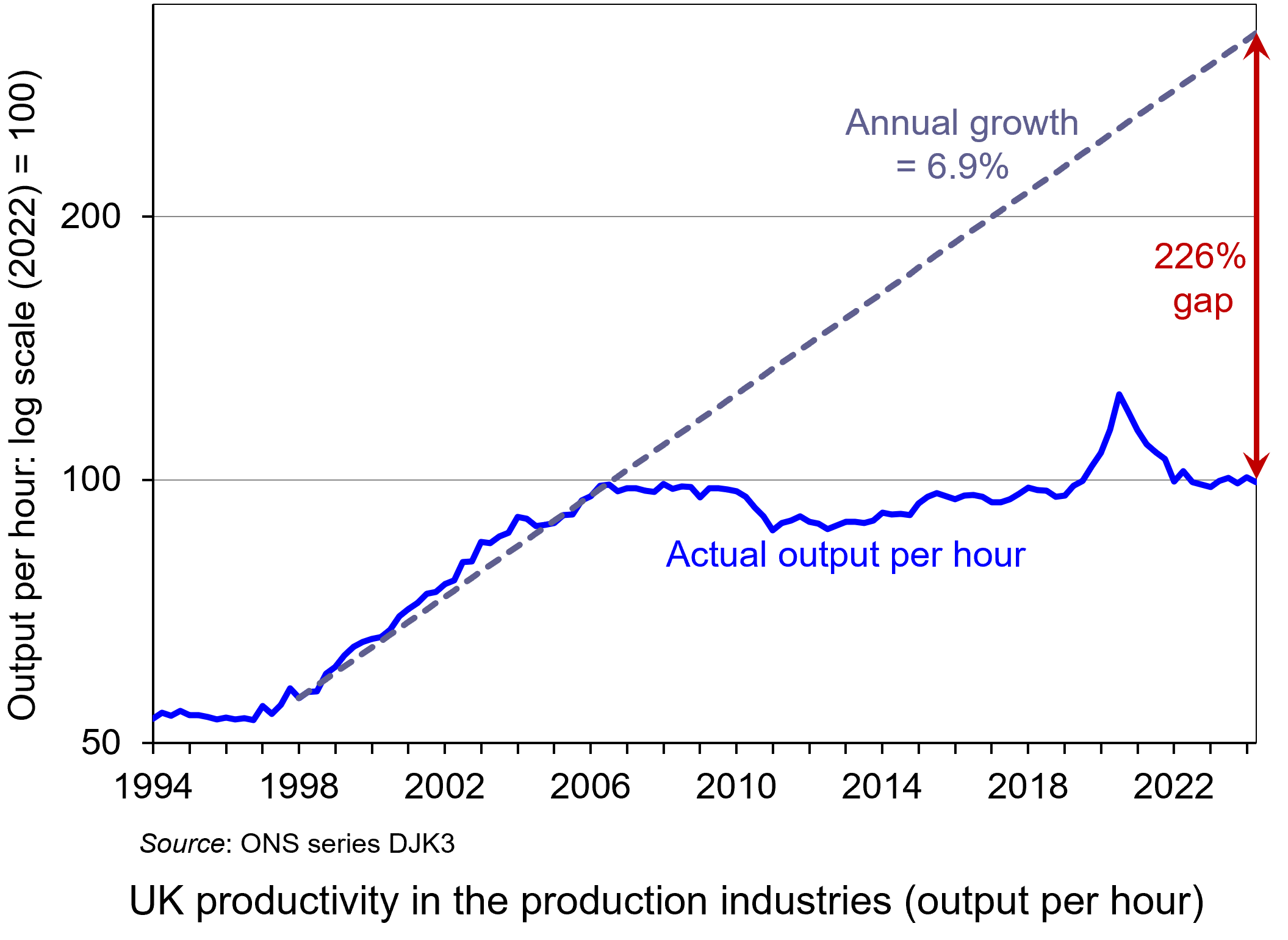 Since the financial crisis of 2007–8, the growth in UK productivity has been sluggish. This is illustrated in the chart, which looks at the production industries: i.e. it excludes services, where average productivity growth tends to be slower. The chart has been updated to 2024 Q2 – the latest data available. (Click here for a PowerPoint of the chart.)
Prior to the crisis, from 1998 to 2006, UK productivity in the production industries grew at an annual rate of 6.9%. From 2007 to the start of the pandemic in 2020, the average annual productivity growth rate in these industries was a mere 0.2%.
It grew rapidly for a short time at the start of the pandemic, but this was because many businesses temporarily shut down or went to part-time working, and many of these temporary job cuts were low-wage/low productivity jobs. If you take services, the effect was even stronger as sectors such as hospitality, leisure and retail were particularly affected and labour productivity in these sectors tends to be low. As industries opened up and took on more workers, so average productivity rapidly fell back. Since then productivity has flatlined.
If you project the average productivity growth rate from 1998 to 2007 of 6.9% forwards (see grey dashed line), then by 2024 Q3, output per hour in the production industries would have been 3.26 times higher than it actually was: a gap of 226%. This is a huge productivity gap.
 Productivity in the UK is lower than in many other competitor countries. According to the ONS, output per hour in the UK in 2021 was $59.14 in the UK. This compares with an average of $64.93 for the G7 countries, $66.75 in France, £68.30 in Germany, $74.84 in the USA, $84.46 in Norway and $128.21 in Ireland. It is lower, however, in Italy ($54.59), Canada ($53.97) and Japan ($47.28).
As we saw in the blog, The UK’s poor productivity record, low UK productivity is caused by a number of factors, not least the lack of investment in physical capital, both by private companies and in public infrastructure, and the lack of investment in training. Other factors include short-termist attitudes of both politicians and management and generally poor management practices. But one cause is the poor motivation of many workers and the feeling of being overworked. One solution to this is the four-day week.
Latest evidence on the four-day week
Results have just been released of a pilot programme involving 61 companies and non-profit organisations in the UK and nearly 3000 workers. They took part in a six-month trial of a four-day week, with no increase in hours on the days worked and no loss in pay for employees – in other words, 100% of the pay for 80% of the time. The trial was a success, with 91% of organisations planning to continue with the four-day week and a further 4% leaning towards doing so.
 The model adopted varied across companies, depending on what was seen as most suitable for them. Some gave everyone Friday off; others let staff choose which day to have off; others let staff work 80% of the hours on a flexible basis.
There was little difference in outcomes across different types of businesses. Compared with the same period last year, revenues rose by an average of 35%; sick days fell by two-thirds and 57% fewer staff left the firms. There were significant increases in well-being, with 39% saying they were less stressed, 40% that they were sleeping better; 75% that they had reduced levels of burnout and 54% that it was easier to achieve a good work–life balance. There were also positive environmental outcomes, with average commuting time falling by half an hour per week.
There is growing pressure around the world for employers to move to a four-day week and this pilot provides evidence that it significantly increases productivity and well-being.
Additional articles
Original set of articles
- Results from world’s largest 4 day week trial bring good news for the future of work
4 Day Week Global, Charlotte Lockhart (21/2/23)
- Four-day week: ‘major breakthrough’ as most UK firms in trial extend changes
The Guardian, Heather Stewart (21/2/23)
- Senedd committee backs four-day working week trial in Wales
The Guardian, Steven Morris (24/1/23)
- ‘Major breakthrough’: Most firms say they’ll stick with a four-day working week after successful trial
Sky News, Alice Porter (21/2/23)
- Major four-day week trial shows most companies see massive staff mental health benefits and profit increase
Independent, Anna Wise (21/2/23)
- Four-day week: Which countries have embraced it and how’s it going so far?
euronews, Josephine Joly and Luke Hurst (23/2/23)
- Firms stick to four-day week after trial ends
BBC News, Simon Read, Lucy Hooker & Emma Simpson (21/2/23)
- The climate benefits of a four-day workweek
BBC Future Planet, Giada Ferraglioni and Sergio Colombo (21/2/23)
- Four-day working week: why UK businesses and workers will continue with new work pattern, plus pros and cons
National World, Rochelle Barrand (22/2/23)
- Most companies in UK four-day week trial to continue with flexible working
Financial Times, Daniel Thomas and Emma Jacobs (21/2/23)
- The pros and cons of a four-day working week
Financial Times, Editorial (13/2/23)
- Explaining the UK’s productivity slowdown: Views of leading economists
VoxEU, Ethan Ilzetzki (11/3/20)
- Why the promised fourth industrial revolution hasn’t happened yet
The Conversation, Richard Markoff and Ralf Seifert (27/2/23)
Questions
- What are the possible advantages of moving to a four-day week?
- What are the possible disadvantages of moving to a four-day week?
- What types of companies or organisations are (a) most likely, (b) least likely to gain from a four-day week?
- Why has the UK’s productivity growth been lower than that of many of its major competitors?
- Why, if you use a log scale on the vertical axis, is a constant rate of growth shown as a straight line? What would a constant rate of growth line look like if you used a normal arithmetical scale for the vertical axis?
- Find out what is meant by the ‘fourth industrial revolution’. Does this hold out the hope of significant productivity improvements in the near future? (See, for example, last link above.)
 The UK government announced on 14 October 2024 in a ministerial statement that it intended to raise the threshold for the ring-fencing (separation) of retail and investment banking activities of large UK-based banks. These banks are known as ‘systemically important financial institutions (SIFIs)’, which are currently defined as those with more than £25bn of core retail deposits. Under the new regulations, the threshold would rise from £25bn to £35bn.
Ring-fencing is the separation of one set of banking services from another. This separation can be geographical or functional. The UK adopted the latter approach, where ring-fencing is the separation of core retail banking services, such as taking deposits, making payments and granting loans to small and medium-sized enterprises (SMEs) from investment banking and international operations. The intention of ring-fencing was to prevent contagion – to protect essential retail banking services from the risks involved in investment banking activities.
Reducing regulation to increase competition
Raising the limit is intended to facilitate greater competition in the retail banking sector. In recent years, US banks, such as JP Morgan and Goldman Sachs, have been expanding their depositor base in the UK under their respective brands – Chase UK and Marcus.
These relatively small UK subsidiaries were not ring-fenced from their wider investment banking operations as their retail deposits were under (but not far under) the £25bn limit. However, this restricted their ability to increase market share further without bearing the additional regulatory burden associated with ring-fencing that much larger incumbents face. Raising the threshold would allow them to expand to the higher limit without the regulatory burden.
The proposals are part of a broader package of reforms aimed at reducing the regulatory burden on UK-based banks. The hope is that this will stimulate greater lending to SMEs to boost investment and productivity.
The proposals also include a new ‘secondary’ threshold. This will exempt banks providing primarily retail banking services from the rules governing the provision of investment banking accounts. This exemption will apply as long as their investment banking is less than 10% of their tier 1 capital. (Tier 1 capital is currently the buffer which banks are required to retain in case of a crisis.) The changes were the outcome of a review conducted in 2022 but had not been implemented by the previous government.
The announcement has sparked a debate about ring-fencing, with some commentators calling for it to be removed altogether. Therefore, it is timely to revisit the rationale for ring-fencing. This blog examines what ring-fencing is and why it was introduced, and explains the associated economic costs and benefits.
Why was ring-fencing introduced?
 Ring-fencing was recommended by the Independent Commission on Banking (ICB) in 2011 (see link below) and implemented through the Financial Services (Banking Reform) Act of 2013. The proposed separation of core retail banking services from investment banking were intended to address issues in banks which arose during the global financial crisis and which required substantial taxpayer bailouts. (See the 2011 blog, Taking the gambling out of high street banking (update).)
Following deregulation and liberalisation of financial services in the 1980s, many UK banks had extended their operations so that they combined domestic retail operations with substantial investment and international operations. The intention was to open up all dimensions of financial services to greater competition and allow banks to exploit economies of scope between retail and investment banking.
However, the risks associated with these services are very different but, in the period before the financial crisis, were provided alongside one another within banking groups.
One significant risk which was not fully recognised at the time was contagion – problems in one dimension of a bank’s activity could severely compromise its ability to provide services in other areas. This is what happened during the financial crisis. Many of the UK banks’ investment operations had made significant investments in off-balance sheet securitised debt instruments – CDOs being the most famous example. (See the 2018 blog, Lehman Brothers: have we learned the lessons 10 years on?.)
 When that market crashed in 2007, several UK-based banks incurred significant losses, as did other banks around the world. Given their thin equity buffers and the inability to borrow due to a credit crunch, such banks found it impossible to bear these losses.
The UK government had to step in to save these institutions from failing. If it had not, there would have been significant economic and social costs associated with their inability to provide core retail banking functions. (See the 2017 blog, Ten years on.)
The Independent Commission proposed that ‘the risks inevitably associated with banking have to sit somewhere, and it should not be with taxpayers. Nor do ordinary depositors have the incentive (given deposit insurance to guard against runs) or the practical ability to monitor or bear those risks’ (p.9). Unstructured banks, with no separation of retail from investment activities, increase the potential for both of these stakeholder groups to bear the risks of investment banking.
Structural separation of retail and investment banking addresses this problem. First, separation should make it easier and less costly to resolve problems for banks that get into trouble, avoiding the need for taxpayer bailouts. Second, structural separation should help to insulate retail banking from external financial shocks, ensuring that customer deposits and essential banking services are protected.
Problems of ring-fencing
Ring-fencing has been subject to criticism, however, which has led to calls for it to be scrapped.
 It must be noted that most of the criticism comes from banks themselves. They state that it required significant operational restructuring by UK banks subject to the regulatory framework which was complex and costly.
In addition, segregating activities can lead to inefficiencies, as banks may not be able to take full advantage of economies of scope between investment and retail banking. Furthermore, ring-fencing could lead to a misallocation of capital, where resources are trapped in one part of the bank and cannot be used to invest in other areas, potentially increasing the risks of the specific areas.
Assessing the new proposals
It is argued that the increased threshold proposed by the authorities may put UK institutions at a competitive disadvantage to outside entrants that are building market share from a low base. Smaller entrants do not have to engage in the costly restructuring that the larger UK incumbents have. They can exploit scope economies and capital mobility within their international businesses to cross-subsidise their retail services in the UK which incumbents with larger deposit-bases are not able to.
However, the UK market for retail banking has significant barriers to entry. Following the acquisition of Virgin Money by Nationwide, only six banking groups in the UK meet the current threshold (Barclays, HSBC, Lloyds Banking Group, NatWest Group, Santander UK and TSB). Indeed, all of those have deposits well above the proposed £35bn threshold. Consequently, raising the threshold should not add significant compliance and efficiency costs, while the potential benefits of greater competition for depositors and SMEs could be a substantial boost to investment and productivity. Furthermore, if the new US entrants do suffer problems, it will not be UK taxpayers who will be liable.
Have we been here before?
In many ways, ring-fencing is a throwback to a previous age of regulation.
 One of the most famous Acts of Congress relating to finance and financial markets in the USA is the Glass-Steagall Act of 1933. The Act was passed in the aftermath of the 1929 Wall Street crash and the onset of the Great Depression in the USA. That witnessed significant bank failures across the country and problems were traced back to significant losses made by banks in their lending to investors during the speculative frenzy that preceded the stock market crash of 1929.
To prevent a repeat of the contagion and ensure financial stability, Glass-Steagall legislated to separate retail banks and investment banks.
In the UK, such separation had long existed due to the historical restrictions placed on investment banks operating in the City of London. In the late 20th century, the arguments for separation became outweighed by arguments for the liberalisation of markets to improve efficiency and competition in financial services. Banking was increasingly deregulated and separation disappeared as retail banks increasingly engaged in investment activities.
That cycle of deregulation reached its nadir in 2007 with the international financial crisis. The need to bail out banks made it clear that the supposed synergies between investment and retail banking were no compensation for the high costs of contagion in the financial system.
Regulators must be wary of calls for the removal of ring-fencing. Sir John Vickers (chairman of the independent commission on banking) highlighted the need to protect depositors, and more importantly taxpayers, from risks in banking. It is the banks that should bear the risks and manage them accordingly. Ultimately, it is up to the banks to do that better.
Articles
Bank annual reports
Access these annual reports to check the deposit base of these UK banks:
Information
Report
- Final Report: Recommendations
The Independent Commission on Banking, Sir John Vickers (Chair), Clare Spottiswoode, Martin Taylor, Bill Winters and Martin Wolf (September 2011)
Questions
- How did the structure of UK banks cause contagion risk in the period before the global financial crisis?
- How does ring-fencing aim to address this and protect depositors and taxpayers?
- Use the links to the annual reports of the covered banks to assess the extent of deposits held by the institutions in 2023. How far above the proposed buffer do the banks sit?
- Use your answer to 3) and economic concepts to analyse the impact on competition in the UK market for retail deposits of raising the threshold.
- What are the risks for financial stability of raising the threshold?
 The market for crude oil is usually a volatile one. Indeed, in the last few months, the market has seen prices rise and fall due to various supply and demand influences. Crude oil is coined the ‘King of Commodities’ due to the impact it has on consumers, producers and both the micro and macro economy. The price of crude oil affects everything from the cost of producing plastics, transportation, and food at the supermarket.
This makes the market for crude oil an economic powerhouse which is closely watched by businesses, traders, and governments. To gain a full understanding of the movements in this market, it is important to identify how demand and supply affect the price of crude oil.
What influences the demand and supply of crude oil?
The law of demand and supply states that if demand increases, prices will rise, and if supply increases, prices will fall. This is exactly what happens in the market for crude oil. The consumer side of the market consists of various companies and hundreds of millions of people. The producer side of the market is made up of oil-producing countries. Collectively, both consumers and producers influence the market price.
However, the demand and supply of crude oil, and therefore the price, is also affected by global economic conditions and geopolitical tensions. What happens in the world impacts the price of oil, especially since a large proportion of the world’s biggest oil producers are in politically unstable areas.
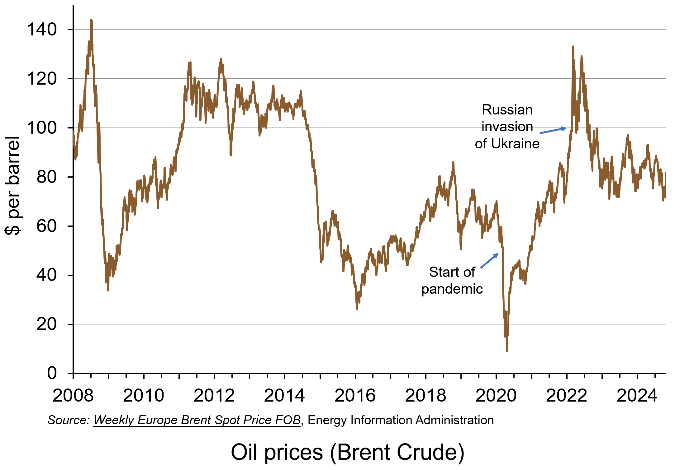 Over the past five years, global events have had a major impact on the price of oil. The economic conditions created by the impact of the COVID pandemic saw prices plummet from around $55 per barrel just before the pandemic in February 2020 to around $15 per barrel in April 2020. By mid-2021 they had recovered to around $75 per barrel. Then, in the aftermath of Russia’s invasion of Ukraine in February 2022, the price surged to reach $133 in June 2022. More recently, geopolitical tensions in the Middle East and concerns about China’s economic outlook have intensified concerns about the future direction of the market. (Click here for a PowerPoint of the chart.)
Geopolitical tensions
In the first week of October 2024, the price of crude oil rose by almost 10% to around $78 per barrel as the conflict in the Middle East intensified. It unfortunately comes at a time when many countries are starting to recover from the rise in oil prices caused by the pandemic and the war in Ukraine. Any increase in prices will affect the price that consumers pay to fill up their vehicles with fuel, just when prices of diesel and petrol had reached their lowest level for three years.
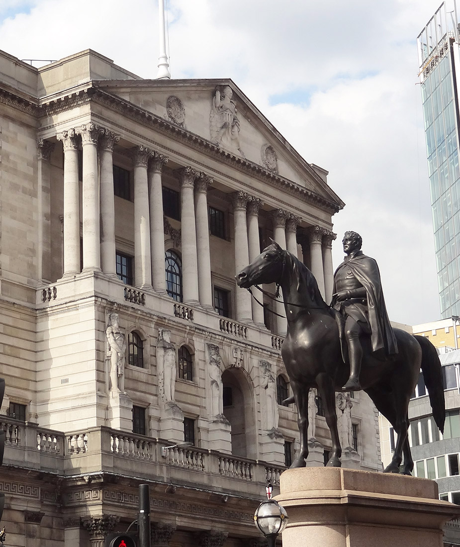 The Governor of the Bank of England, Andrew Bailey, has said that the Bank is monitoring developments in the Middle East ‘extremely closely’, as the conflict has the potential to have serious impacts in the UK. The Bank of England will therefore be watching for any movement in oil prices that could fuel inflation.
The main concerns stem from further escalation in the conflict between Israel and the Iran-backed armed group, Hezbollah, in Lebanon. If Israel decides to attack Iran’s oil sector, this is likely to cause a sharp rise in the price of oil. Iran is the world’s seventh largest oil exporter and exports over half of its production to China. If the oilfields of a medium-sized supplier, like Iran, were attacked, this could threaten general inflation in the UK, which could in turn influence any decision by the Bank of England to lower interest rates next month.
Supply deficits
This week (2nd week of October 2024) saw the price of crude oil surge above $81 per barrel to hit its highest level since August. This rise means that prices increased by 12% in a week. However, this surge in price also means that prices rose by almost 21% between the start September and the start of October alone. Yet it was only in early September when crude oil hit a year-to-date low, highlighting the volatility in the market.
As the Middle-East war enters a new and more energy-related phase, the loss of Iranian oil would leave the market in a supply deficit. The law of supply implies that such a deficit would lead to an increase in prices. This also comes at a time when the US Strategic Petroleum Reserve has also been depleted, causing further concerns about global oil supply.
 However, the biggest and most significant impact would be a disruption to flows through the Strait of Hormuz. This is a relatively narrow channel at the east end of the Persian Gulf through which a huge amount of oil tanker traffic passes – about a third of total seaborne-traded oil. It is therefore known as the world’s most important oil transit chokepoint. The risk that escalation could block the Strait of Hormuz could technically see a halt in about a fifth of the world’s oil supply. This would include exports from big Gulf producers, including Saudi Arabia, UAE, Kuwait and Iraq. In a worst-case scenario of a full closure of the Strait, a barrel of oil could very quickly rise to well above $100.
Disruption to shipments would also lead to higher gas prices and therefore lead to a rise in household gas and electricity bills. As with oil, gas prices filter down supply chains, affecting the cost of virtually all goods, resulting in a further rise in the cost of living. With energy bills in the UK having already risen by 10% for this winter, an escalation to the conflict could see prices rise further still.
China’s economic outlook

Despite the concern for the future supply of oil, there is also a need to consider how the demand for oil could impact price changes in the market. The price of oil declined on 14 October 2024 in light of concerns over China’s struggling economy. As China is the world’s largest importer of crude oil, there are emerging fears about the potential limits on fuel demand. This fall in price reversed increases made the previous week as investors become concerned about worsening deflationary pressures in China.
Any reduced demand from China could indicate an oversupply of crude oil and therefore potential price declines. Official data from China reveal a sharp year-on-year drop in the producer price index of 2.8% – the fastest decline in six months. These disappointing results have stirred uncertainty about the Chinese government’s economic stimulus plans. Prices could fall further if there are continuing doubts about the government’s ability to implement effective fiscal measures to promote consumer spending and, in turn, economic growth.
As a result of the 2% price fall in oil prices on 14 October, OPEC (the Organization of the Petroleum Exporting Countries) has lowered its 2024 and 2025 global oil demand growth. This negative news outweighed market concerns over the possibility that an Israeli response to Iran’s missile attack could disrupt oil production.
What is the future for oil prices?
 It is expected that the market for oil will remain a volatile one. Indeed, the current uncertainties around the globe only highlight this. It is never a simple task to predict what will happen in a market that is influenced by so many global factors, and the current global landscape only adds to the complexity.
There’s a wide spectrum of predictions about what could come next in the market for crude oil. Given the changes in the first two weeks of October alone, supply and demand factors from separate parts of the globe have made the future of oil prices particularly uncertain. Callum Macpherson, head of commodities at Investec, stated in early October that ‘there is really no way of telling where we will be this time next week’ (see the first BBC News article linked below).
Despite the predominately negative outlook, this is all based on potential scenarios. Caroline Bain, chief commodities economist at Capital Economics suggests that if the ‘worst-case scenario’ of further escalation in the Middle East conflict does not materialise, oil prices are likely to ‘ease back quite quickly’. Even if Iran’s supplies were disrupted, China could turn to Russia for its oil. Bain says that there is ‘more than enough capacity’ globally to cover the gap if Iranian production is lost. However, this does then raise the question of where the loyalty of Saudi Arabia, the world’s second largest oil producer, lies and whether it will increase or restrict further production.
What is certain is that the market for crude oil will continue to be a market that is closely observed. It doesn’t take much change in global activity for prices to move. Therefore, in the current political and macroeconomic environment, the coming weeks and months will be critical in determining oil prices and, in turn, their economic effects.
Articles
- How worried should I be about rising oil prices?
BBC News, Michael Race (4/10/24)
- Interest rates could fall more quickly, hints Bank
BBC News, Dearbail Jordan (3/10/24)
- Oil Prices Eye $100 A Barrel As War Risk Premium Returns
FX Empire, Phil Carr (8/10/24)
- Crude oil futures reverse previous gains following disappointing economic data from China
London Loves Business, Hamza Zraimek (14/10/24)
- Oil falls 2% as OPEC cuts oil demand growth view, China concerns
Reuters, Arathy Somasekhar (14/10/24)
- Could war in the Gulf push oil to $100 a barrel?
The Economist (7/10/24)
- The Commodities Feed: Oil remains volatile
ING Think, Ewa Manthey and Warren Patterson (8/10/24)
- Who and what is driving oil price volatility
FT Alphaville, George Steer (9/10/24)
- Brent crude surges above $80 as conflict and storm spark supply fears
Financial Times, Rafe Uddin and Jamie Smyth (7/10/24)
Questions
- Use a demand and supply diagram to illustrate what has happened to oil prices in the main two scenarios:
(a) Conflict in the Middle East;
(b) Concerns about China’s economic performance.
- How are the price elasticities of demand and supply relevant to the size of any oil price change?
- What policy options do the governments have to deal with the potential of increasing energy prices?
- What are oil futures? What determines oil future prices?
- How does speculation affect oil prices?
 We continue to live through incredibly turbulent times. In the past decade or so we have experienced a global financial crisis, a global health emergency, seen the UK’s departure from the European Union, and witnessed increasing levels of geopolitical tension and conflict. Add to this the effects from the climate emergency and it easy to see why the issue of economic uncertainty is so important when thinking about a country’s economic prospects.
In this blog we consider how we can capture this uncertainty through a World Uncertainty Index and the ways by which economic uncertainty impacts on the macroeconomic environment.
World Uncertainty Index
Hites Ahir, Nicholas Bloom and Davide Furceri have constructed a measure of uncertainty known as the World Uncertainty Index (WUI). This tracks uncertainty around the world using the process of ‘text mining’ the country reports produced by the Economist Intelligence Unit. The words searched for are ‘uncertain’, ‘uncertainty’ and ‘uncertainties’ and a tally is recorded based on the number of times they occur per 1000 words of text. To produce the index this figure is then multiplied up by 100 000. A higher number therefore indicates a greater level of uncertainty. For more information on the construction of the index see the 2022 article by Ahir, Bloom and Furceri linked below.
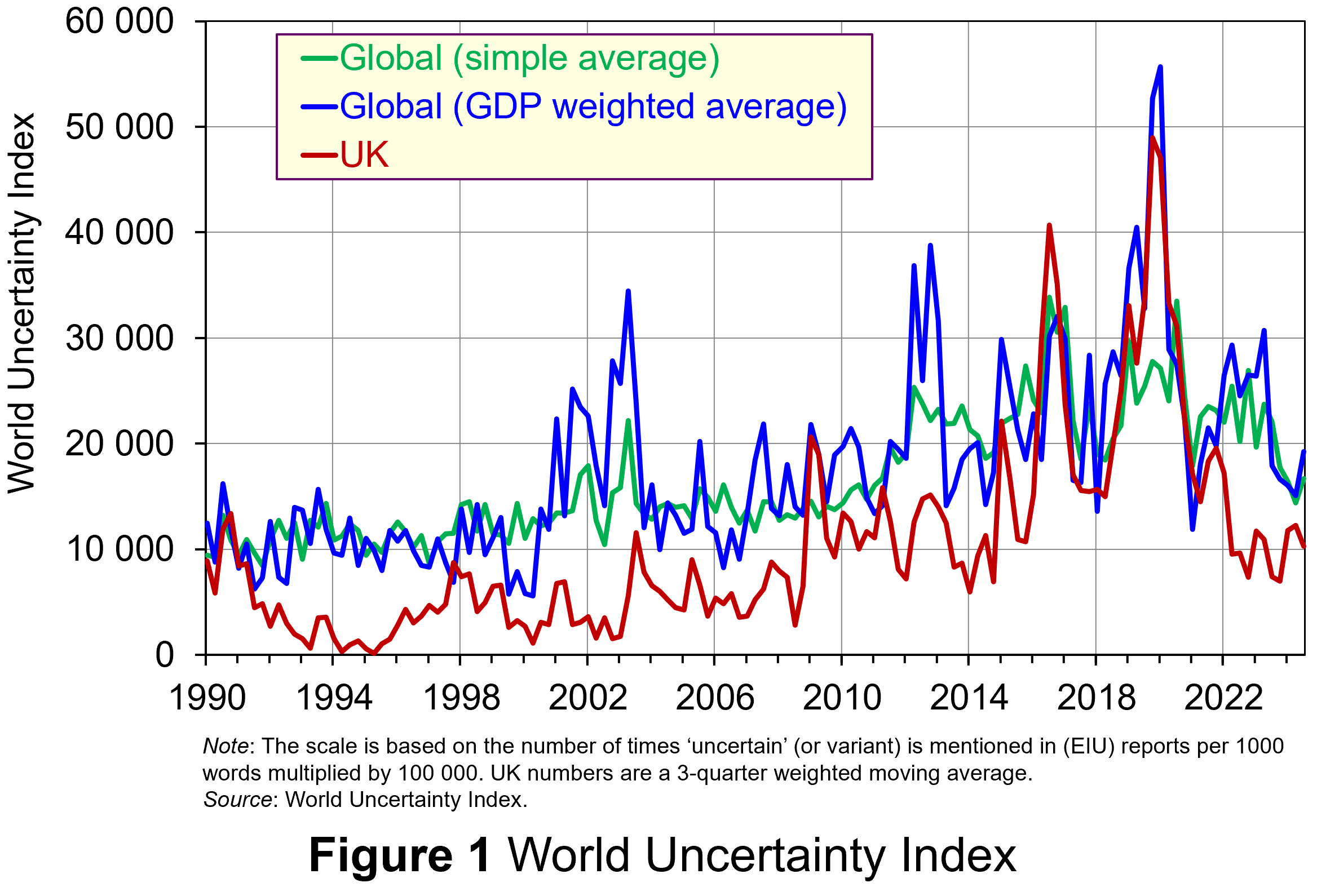 Figure 1 (click here for a PowerPoint) shows the WUI both globally and in the UK quarterly since 1991. The global index covers 143 countries and is presented as both a simple average and a GDP weighted average. The UK WUI is also shown. This is a three-quarter weighted average, the authors’ preferred measure for individual countries, where increasing weights of 0.1, 0.3 and 0.6 are used for the three most recent quarters.
From Figure 1 we can see how the level of uncertainty has been particularly volatile over the past decade or more. Events such as the sovereign debt crisis in parts of Europe in the early 2010s, the Brexit referendum in 2016, the COVID-pandemic in 2020–21 and the invasion of Ukraine in 2022 all played their part in affecting uncertainty domestically and internationally.
Uncertainty, risk-aversion and aggregate demand
Now the question turns to how uncertainty affects economies. One way of addressing this is to think about ways in which uncertainty affects the choices that people and businesses make. In doing so, we could think about the impact of uncertainty on components of aggregate demand, such as household consumption and investment, or capital expenditures by firms.
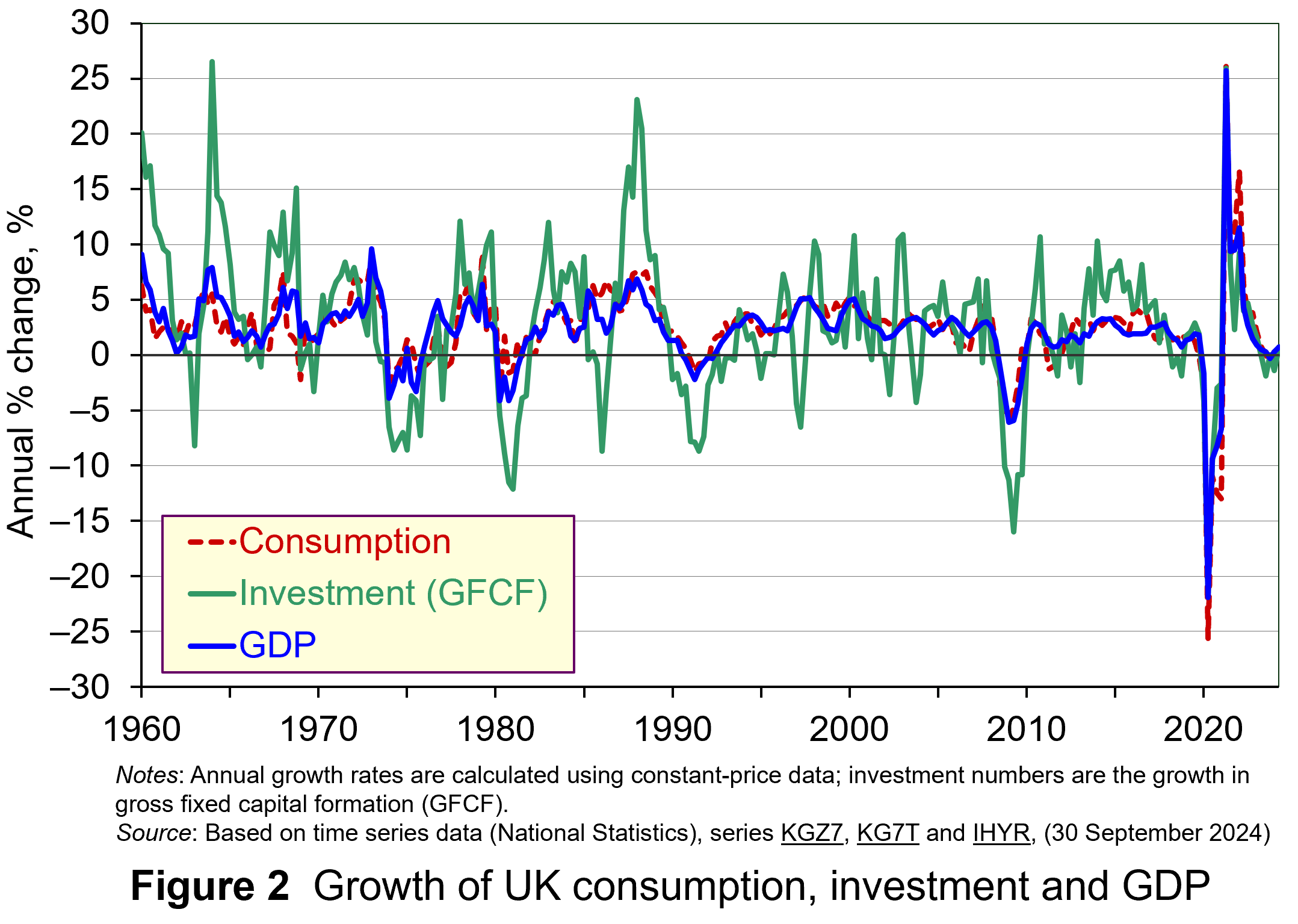 As Figure 2 shows (click here for a PowerPoint), investment is particularly volatile, and much more so than household spending. Some of this can be attributed to the ‘lumpiness’ of investment decisions since these expenditures tend to be characterised by indivisibility and irreversibility. This means that they are often relatively costly to finance and are ‘all or nothing’ decisions. In the context of uncertainty, it can make sense therefore for firms to wait for news that makes the future clearer. In this sense, we can think of uncertainty rather like a fog that firms are peering through. The thicker the fog, the more uncertain the future and the more cautious firms are likely to be.
The greater caution that many firms are likely to adopt in more uncertain times is consistent with the property of risk-aversion that we often attribute to a range of economic agents. When applied to household spending decisions, risk-aversion is often used to explain why households are willing to hold a buffer stock of savings to self-insure against unforeseen events and their future financial outcomes being worse than expected. Hence, in more uncertain times households are likely to want to increase this buffer further.
 The theory of buffer-stock saving was popularised by Christopher Carroll in 1992 (see link below). It implies that in the presence of uncertainty, people are prepared to consume less today in order to increase levels of saving, pay off existing debts, or borrow less relative to that in the absence of uncertainty. The extent of the buffer of financial wealth that people want to hold will depend on their own appetite for risk, the level of uncertainty, and the moderating effect from their own impatience and, hence, present bias for consuming today.
Risk aversion is consistent with the property of diminishing marginal utility of income or consumption. In other words, as people’s total spending volumes increase, their levels of utility or satisfaction increase but at an increasingly slower rate. It is this which explains why individuals are willing to engage with the financial system to reallocate their expected life-time earnings and have a smoother consumption profile than would otherwise be the case from their fluctuating incomes.
Yet diminishing marginal utility not only explains consumption smoothing, but also why people are willing to engage with the financial system to have financial buffers as self-insurance. It explains why people save more or borrow less today than suggested by our base-line consumption smoothing model. It is the result of people’s greater dislike (and loss of utility) from their financial affairs being worse than expected than their like (and additional utility) from them being better than expected. This tendency is only likely to increase the more uncertain times are. The result is that uncertainty tends to lower household consumption with perhaps ‘big-ticket items’, such as cars, furniture, and expensive electronic goods, being particularly sensitive to uncertainty.
Uncertainty and confidence
Uncertainty does not just affect risk; it also affects confidence. Risk and confidence are often considered together, not least because their effects in generating and transmitting shocks can be difficult to disentangle.
We can think of confidence as capturing our mood or sentiment, particularly with respect to future economic developments. Figure 3 plots the Uncertainty Index for the UK alongside the OECD’s composite consumer and business confidence indicators. Values above 100 for the confidence indicators indicate greater confidence about the future economic situation and near-term business environment, while values below 100 indicate pessimism towards the future economic and business environments.
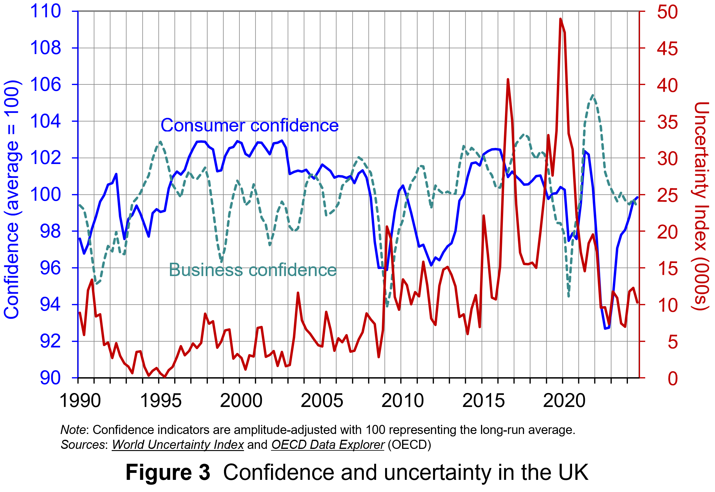 Figure 3 suggests that the relationship between confidence and uncertainty is rather more complex than perhaps is generally understood (click here for a PowerPoint). Haddow, Hare, Hooley and Shakir (see link below) argue that the evidence tends to point to changes in uncertainty affecting confidence, but with less evidence that changes in confidence affect uncertainty.
To illustrate this, consider the global financial crisis of the late 2000s. The argument can be made that the heightened uncertainty about future prospects for households and businesses helped to erode their confidence in the future. The result was that people and businesses revised down their expectations of the future (pessimism). However, although people were more pessimistic about the future, this was more likely to have been the result of uncertainty rather than the cause of further uncertainty.
Conclusion
For economists and policymakers alike, indicators of uncertainty, such as the Ahir, Bloom and Furceri World Uncertainty Index, are invaluable tools in understanding and forecasting behaviour and the likely economic outcomes that follow. Some uncertainty is inevitable, but the persistence of greater uncertainty since the global financial crisis of the late 2000s compares quite starkly with the relatively lower and more stable levels of uncertainty seen from the mid-1990s up to the crisis. Hence the recent frequency and size of changes in uncertainty show how important it to understand how uncertainty effects transmit through economies.
Academic papers
- The World Uncertainty Index
National Bureau of Economic Research, Working Paper 29763, Hites Ahir, Nicholas Bloom and Davide Furceri (February 2022)
- The Buffer-Stock Theory of Saving: Some Macroeconomic Evidence
Brookings Papers on Economic Activity, Christopher D Carroll (Vol 2, 1992)
- Macroeconomic uncertainty: what is it, how can we measure it and why does it matter?
Bank of England Quarterly Bulletin, 2013 Q2, Abigail Haddow, Chris Hare, John Hooley and Tamarah Shakir (13/6/13)
Articles
Data
Questions
- (a) Explain what is meant by the concept of diminishing marginal utility of consumption.
(b) Explain how this concept helps us to understand both consumption smoothing and the motivation to engage in buffer-stock saving.
- Explain the distinction between confidence and uncertainty when analysing macroeconomic shocks.
- Discuss which types of expenditures you think are likely to be most susceptible to uncertainty shocks.
- Discuss how economic uncertainty might affect productivity and the growth of potential output.
- How might the interconnectedness of economies affect the transmission of uncertainty effects through economies?
 In the second of a series of blogs looking at applications of the distinction between nominal and real indicators, we revisit the blog Getting Real with Growth last updated in October 2021.
In this blog, we discuss how, in making a meaningful comparison over time of a country’s national income and, therefore, the aggregate purchasing power of its people, we need to take inflation into account. Likewise, if we want to analyse changes in the volume of production, we need to eliminate the effects of price changes on GDP. This is important when analysing the business cycle and identifying periods of boom or bust. Hence, in this updated blog we take another look at what real GDP data reveal about both longer-term economic growth and the extent of economic volatility – or what we refer to as the twin characteristics of economic growth.
Real and nominal GDP
The nominal (or current-price) estimate for UK gross domestic product in 2023 was £2.687 trillion. The estimate of national output or national income is based primarily on the production of final goods and services and, hence, purchased by the final user. It therefore largely excludes intermediate goods and services: i.e. goods and services that are transformed or used up in the process of making something else, although data on imports and exports do include intermediate goods and services. The 2023 figure represents a nominal increase in national income of 7.2 per cent on the £2.51 trillion recorded in 2022. These values make no adjustment for inflation and therefore reflect the prices of output that were prevailing at the time.
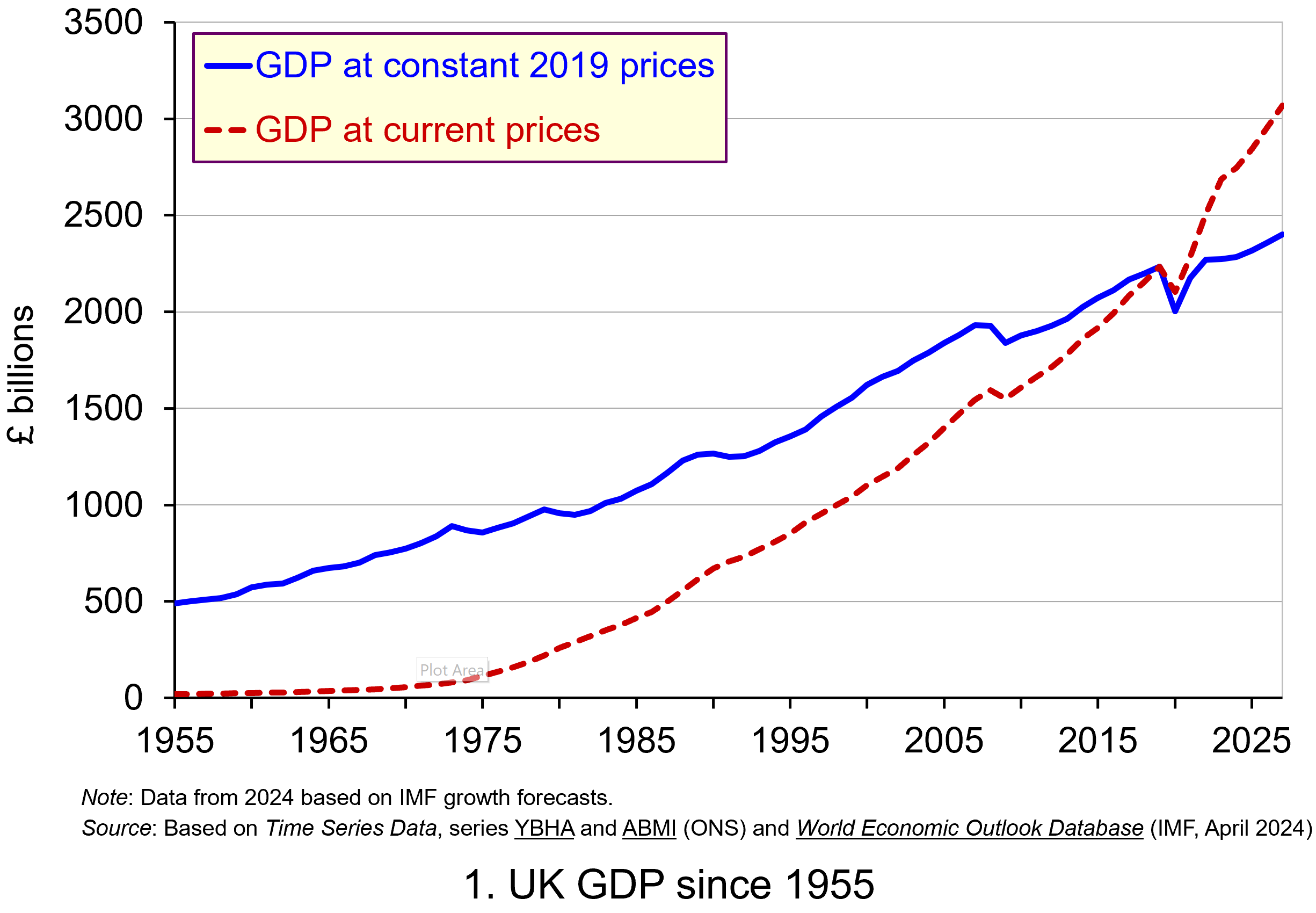 Chart 1 shows current-price estimates of GDP from 1955, when the value of GDP was estimated at £19.2 billion. The £2.687 trillion figure recorded for 2023 is an increase of over 140 times that in 1955, a figure that rises to 160 times if we compare the 1950 value with the latest IMF estimate for 2027. However, if we want to make a more meaningful comparison of the country’s national income we need to adjust for inflation. (Click here to download a PowerPoint of the chart.)
Long-term growth in real GDP
If we measure GDP at constant prices, we eliminate the effect of inflation. To construct a constant-price series for GDP, a process known as chain-linking is used. This involves taking consecutive pairs of years, e.g. 2022 and 2023, and estimating what GDP would be in the most recent year (in this case, 2023) if the previous year’s prices (i.e. 2022) had continued to prevail. By calculating the percentage change from the previous year’s GDP value we have an estimate of the volume change. If this is repeated for other pairs of years, we have a series of percentage changes that capture the volume changes from year-to-year. Finally, a reference year is chosen and the percentage volume changes are applied backwards and forwards from the nominal GDP value for the reference year.
In effect, a real GDP series creates a quantity measure in monetary terms. Chart 1 shows GDP at constant 2019 prices (real GDP) alongside GDP at current prices (nominal GDP). Consider first the real GDP numbers for 1955 and 2023. GDP in 1950 at 2019 prices was £491.2 billion. This is higher than the current-price value because prices in 2019 (the reference year) were higher than those in 1955. Meanwhile, GDP in 2023 when measured at 2019 prices was £2.273 trillion. This constant-price value is smaller than the corresponding current-price value because prices in 2019 where lower than those in 2023.
 Between 1955 and 2023 real GDP increased 4.6 times. If we extend the period to 2027, again using the latest IMF estimates, the increase is 4.9 times. Because we have removed the effect of inflation, the real growth figure is much lower than the nominal growth figure.
Crucially, what we are left with is an indicator of the long-term growth in the volume of the economy’s output and hence an increase in national income that is backed up by an increase in production. Whereas nominal growth rates are affected by changes in both volumes and prices, real growth rates reflect only changes in volumes.
The upward trajectory observed in constant-price GDP is therefore evidence of positive longer-term growth. This is one of the twin characteristics of growth.
Short-term fluctuations in the growth of real GDP
The second characteristic is fluctuations in the rate of growth from period to period. We can see this second characteristic more clearly by plotting the percentage change in real GDP from year to year.
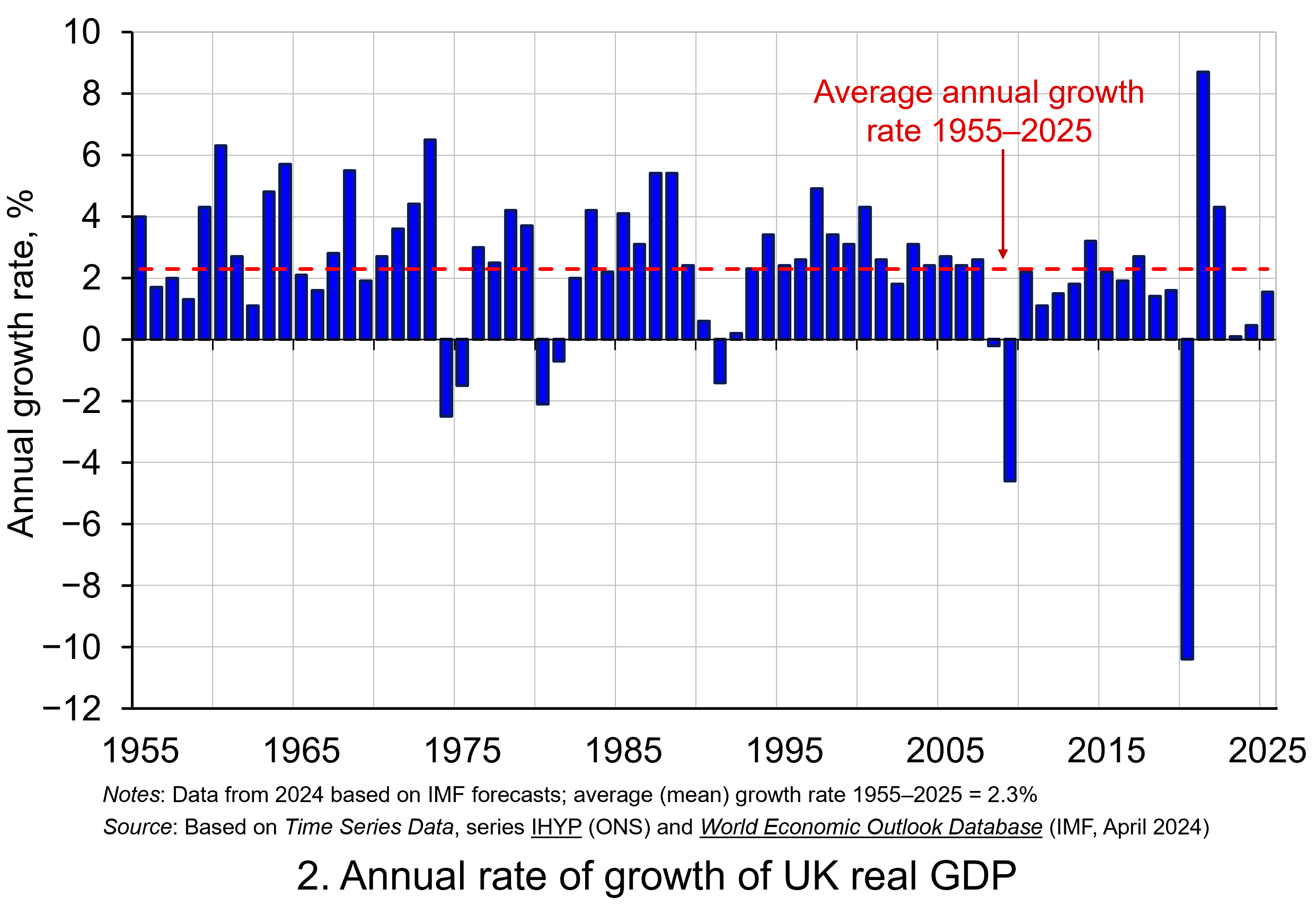 Chart 2 shows the annual rate of growth in real GDP each year from 1955 to 2025. From it, we see the inherent instability that is a key characteristic of the macroeconomic environment. This instability is, of course, mirrored in the output path of real GDP in Chart 1, but the annual rates of growth show the instability more clearly. We can readily see the impact on national output of the global financial crisis of 2007–8 and the global COVID pandemic.
In 2009, constant-price GDP in the UK fell by 4.6 per cent, whereas current-price GDP fell by 2.8 per cent. Then, in 2020, constant-price GDP and, hence, the volume of national output fell by 10.4 per cent, as compared to a 5.8 per cent fall in current-price GDP. These global, ‘once-in-a-generation’ shocks are stark examples of the instability that characterises economies and which generate the ‘ups and downs’ in an economy’s output path, known more simply as ‘the business cycle’. (Click here to download a PowerPoint copy of the chart.)
Determinants of long-and short-term growth
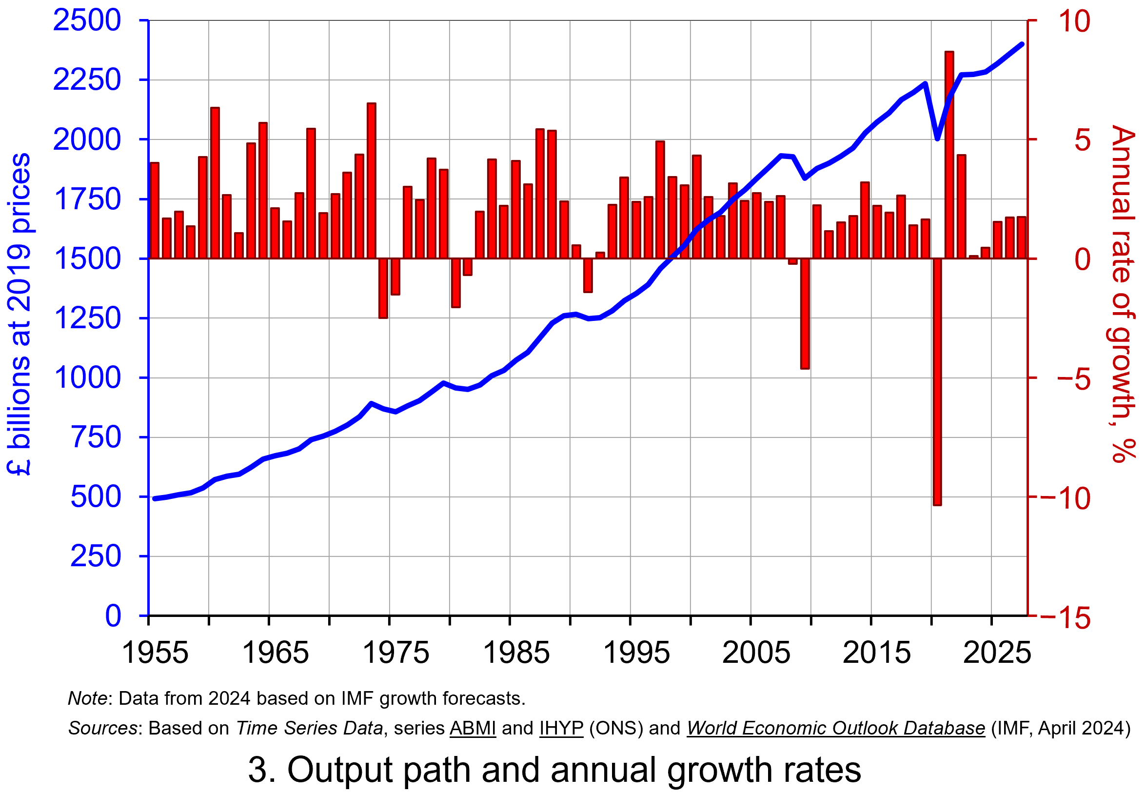 The twin characteristics of growth can be seen simultaneously by combining the output path (shown by the levels of real GDP) with the annual rates of growth. This is shown in Chart 3. The longer-term growth seen in the economy’s output path is generally argued to be driven by the quantity and quality of the economy’s resources, and their effectiveness when combined in production (i.e. their productivity). In other words, it is the supply side of the economy that determines the trajectory of the output path over the longer term. (Click here to download a PowerPoint copy of the chart.)
However, the fluctuations we observe in short-term growth rates tend to reflect shocks, also known as impulses, that originate either from the ability and or willingness of purchasers to consume (demand-side shocks) or producers to supply (supply-side shocks). These impulses are then amplified (or ‘propagated’) via the multiplier, expectations and other factors, and their effects, therefore, transmitted through the economy. Unusually in the case of the pandemic, the lockdown measures employed by governments around the world resulted in simultaneous negative aggregate demand and aggregate supply shocks.
Persistence effects
Explanations of the business cycle and of long-term growth are not mutually exclusive. The shocks and the propagation mechanisms that help to create and shape the business cycle can themselves have enduring or persistent effects on output. The global financial crisis, fuelled by unsustainable lending and the overstretch of private-sector balance sheets, which then spilt over to the public sector as governments attempted to stabilise the financial system and support aggregate demand, is argued by some to have created the conditions for low-growth persistence seen in many countries in the 2010s. This type of persistence is known as hysteresis as it originates from a negative demand shock.
Economists and policymakers were similarly concerned that the pandemic would also generate persistence in the form of scarring effects that might again affect the economy’s output path. Such concerns help to explain why many governments introduced furlough schemes to protect jobs and employment income, as well as provide grants or loans to business.
Per capita output
To finish, it is important to recognise that, when thinking about living standards, it is the growth in real GDP per capita that we need to consider. A rise in real GDP will only lead to a rise in overall living standards if it is faster than the rise in population.
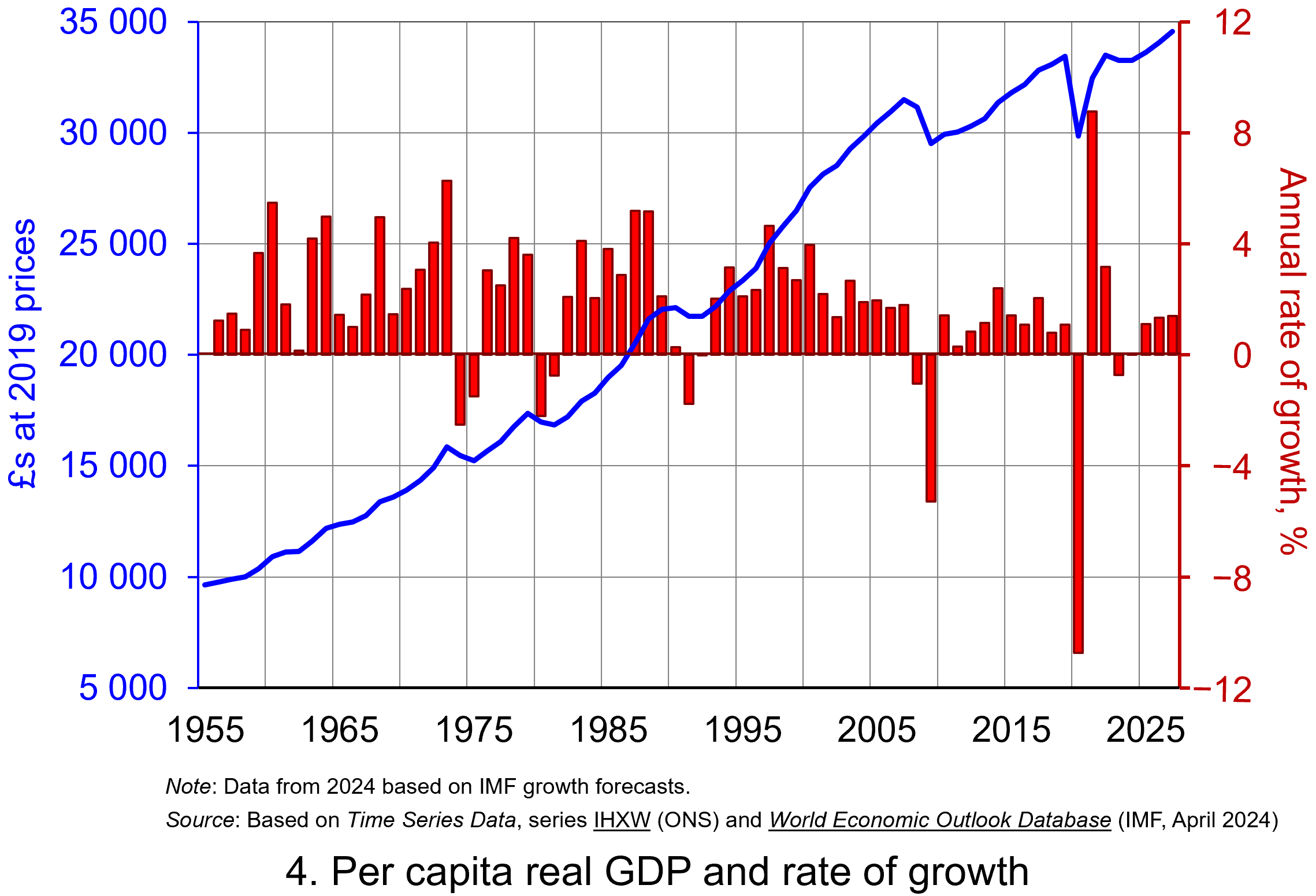 Our final chart therefore replicates Chart 3 but for real GDP per capita. Between 1955 and 2023 real GDP per capita grew by a factor of 3.45, which increases to 3.6 when we consider the period up to 2027. The average rate of growth of real GDP per capita up to 2023 was 1.87 per cent (lower than the 2.34 per cent increase in real GDP).
But the rate of increase in real GDP per capita was much higher before 2007 than it has been since. If we look at the period up to 2007 and, hence, before the global financial crisis, the figure is 2.32 per cent (2.7 per cent for real GDP), whereas from 2008 to 2023 the average rate of growth of real GDP per capita was a mere 0.42 per cent (1.1 per cent for real GDP). (Click here to download a PowerPoint copy of the chart.)
The final chart therefore reiterates the messages from recent blogs, such as Getting Real with Pay and The Productivity Puzzle, that long-term economic growth and the growth of real wages have slowed dramatically since the financial crisis. This has had important implications for the wellbeing of all sectors of the economy. The stagnation of living standards is therefore one of the most important economic issues of our time. It is one that the incoming Labour government will be keen to address.
Data and Reports
Articles
Questions
- What do you understand by the term ‘macroeconomic environment’? What data could be used to describe the macroeconomic environment?
- When a country experiences positive rates of inflation, which is higher: nominal economic growth or real economic growth?
- Does an increase in nominal GDP mean a country’s production has increased? Explain your answer.
- Does a decrease in nominal GDP mean a country’s production has decreased? Explain your answer.
- Why does a change in the growth of real GDP allow us to focus on what has happened to the volume of production?
- What does the concept of the ‘business cycle’ have to do with real rates of economic growth?
- When would falls in real GDP be classified as a recession?
- Distinguish between the concepts of ‘short-term growth’ and ‘longer-term growth’.
- What do you understand by the term ‘persistence’ in macroeconomics? Given examples of persistence effects and the means by which they can be generated?
- Discuss the proposition that the pandemic could have a positive effect on longer-term growth rates because of the ways that people and business have had to adapt.
 In a blog from March 2023 (reproduced below), we saw how there has been growing pressure around the world for employers to move to a four-day week. Increasing numbers of companies have adopted the model of 80% of the hours for 100% of the pay.
 Since the financial crisis of 2007–8, the growth in UK productivity has been sluggish. This is illustrated in the chart, which looks at the production industries: i.e. it excludes services, where average productivity growth tends to be slower. The chart has been updated to 2024 Q2 – the latest data available. (Click here for a PowerPoint of the chart.)
  Productivity in the UK is lower than in many other competitor countries. According to the ONS, output per hour in the UK in 2021 was $59.14 in the UK. This compares with an average of $64.93 for the G7 countries, $66.75 in France, £68.30 in Germany, $74.84 in the USA, $84.46 in Norway and $128.21 in Ireland. It is lower, however, in Italy ($54.59), Canada ($53.97) and Japan ($47.28).
 The model adopted varied across companies, depending on what was seen as most suitable for them. Some gave everyone Friday off; others let staff choose which day to have off; others let staff work 80% of the hours on a flexible basis.
 The UK government announced on 14 October 2024 in a ministerial statement that it intended to raise the threshold for the ring-fencing (separation) of retail and investment banking activities of large UK-based banks. These banks are known as ‘systemically important financial institutions (SIFIs)’, which are currently defined as those with more than £25bn of core retail deposits. Under the new regulations, the threshold would rise from £25bn to £35bn.
 Ring-fencing was recommended by the Independent Commission on Banking (ICB) in 2011 (see link below) and implemented through the Financial Services (Banking Reform) Act of 2013. The proposed separation of core retail banking services from investment banking were intended to address issues in banks which arose during the global financial crisis and which required substantial taxpayer bailouts. (See the 2011 blog,
  When that market crashed in 2007, several UK-based banks incurred significant losses, as did other banks around the world. Given their thin equity buffers and the inability to borrow due to a credit crunch, such banks found it impossible to bear these losses.
 It must be noted that most of the criticism comes from banks themselves. They state that it required significant operational restructuring by UK banks subject to the regulatory framework which was complex and costly.
 One of the most famous Acts of Congress relating to finance and financial markets in the USA is the Glass-Steagall Act of 1933. The Act was passed in the aftermath of the 1929 Wall Street crash and the onset of the Great Depression in the USA. That witnessed significant bank failures across the country and problems were traced back to significant losses made by banks in their lending to investors during the speculative frenzy that preceded the stock market crash of 1929.
 The market for crude oil is usually a volatile one. Indeed, in the last few months, the market has seen prices rise and fall due to various supply and demand influences. Crude oil is coined the ‘King of Commodities’ due to the impact it has on consumers, producers and both the micro and macro economy. The price of crude oil affects everything from the cost of producing plastics, transportation, and food at the supermarket.
 Over the past five years, global events have had a major impact on the price of oil. The economic conditions created by the impact of the COVID pandemic saw prices plummet from around $55 per barrel just before the pandemic in February 2020 to around $15 per barrel in April 2020. By mid-2021 they had recovered to around $75 per barrel. Then, in the aftermath of Russia’s invasion of Ukraine in February 2022, the price surged to reach $133 in June 2022. More recently, geopolitical tensions in the Middle East and concerns about China’s economic outlook have intensified concerns about the future direction of the market. (Click
  The Governor of the Bank of England, Andrew Bailey, has said that the Bank is monitoring developments in the Middle East ‘extremely closely’, as the conflict has the potential to have serious impacts in the UK. The Bank of England will therefore be watching for any movement in oil prices that could fuel inflation.
 However, the biggest and most significant impact would be a disruption to flows through the Strait of Hormuz. This is a relatively narrow channel at the east end of the Persian Gulf through which a huge amount of oil tanker traffic passes – about a third of total seaborne-traded oil. It is therefore known as the world’s most important oil transit chokepoint. The risk that escalation could block the Strait of Hormuz could technically see a halt in about a fifth of the world’s oil supply. This would include exports from big Gulf producers, including Saudi Arabia, UAE, Kuwait and Iraq. In a worst-case scenario of a full closure of the Strait, a barrel of oil could very quickly rise to well above $100.
 It is expected that the market for oil will remain a volatile one. Indeed, the current uncertainties around the globe only highlight this. It is never a simple task to predict what will happen in a market that is influenced by so many global factors, and the current global landscape only adds to the complexity.
 We continue to live through incredibly turbulent times. In the past decade or so we have experienced a global financial crisis, a global health emergency, seen the UK’s departure from the European Union, and witnessed increasing levels of geopolitical tension and conflict. Add to this the effects from the climate emergency and it easy to see why the issue of economic uncertainty is so important when thinking about a country’s economic prospects.
 Figure 1 (click
  As Figure 2 shows (click
  The theory of buffer-stock saving was popularised by Christopher Carroll in 1992 (see link below). It implies that in the presence of uncertainty, people are prepared to consume less today in order to increase levels of saving, pay off existing debts, or borrow less relative to that in the absence of uncertainty. The extent of the buffer of financial wealth that people want to hold will depend on their own appetite for risk, the level of uncertainty, and the moderating effect from their own impatience and, hence, present bias for consuming today.
 Figure 3 suggests that the relationship between confidence and uncertainty is rather more complex than perhaps is generally understood (click
  In the second of a series of blogs looking at applications of the distinction between nominal and real indicators, we revisit the blog
  Chart 1 shows current-price estimates of GDP from 1955, when the value of GDP was estimated at £19.2 billion. The £2.687 trillion figure recorded for 2023 is an increase of over 140 times that in 1955, a figure that rises to 160 times if we compare the 1950 value with the latest IMF estimate for 2027. However, if we want to make a more meaningful comparison of the country’s national income we need to adjust for inflation. (Click
  Between 1955 and 2023 real GDP increased 4.6 times. If we extend the period to 2027, again using the latest IMF estimates, the increase is 4.9 times. Because we have removed the effect of inflation, the real growth figure is much lower than the nominal growth figure.
 Chart 2 shows the annual rate of growth in real GDP each year from 1955 to 2025. From it, we see the inherent instability that is a key characteristic of the macroeconomic environment. This instability is, of course, mirrored in the output path of real GDP in Chart 1, but the annual rates of growth show the instability more clearly. We can readily see the impact on national output of the global financial crisis of 2007–8 and the global COVID pandemic.
 The twin characteristics of growth can be seen simultaneously by combining the output path (shown by the levels of real GDP) with the annual rates of growth. This is shown in Chart 3. The longer-term growth seen in the economy’s output path is generally argued to be driven by the quantity and quality of the economy’s resources, and their effectiveness when combined in production (i.e. their productivity). In other words, it is the supply side of the economy that determines the trajectory of the output path over the longer term. (Click
  Our final chart therefore replicates Chart 3 but for real GDP per capita. Between 1955 and 2023 real GDP per capita grew by a factor of 3.45, which increases to 3.6 when we consider the period up to 2027. The average rate of growth of real GDP per capita up to 2023 was 1.87 per cent (lower than the 2.34 per cent increase in real GDP).