 In this blog we show how we can apply fiscal metrics to assess the UK government’s fiscal stance. This captures the extent to which fiscal policy contributes to the level of economic activity in the economy.
Changes in the fiscal stance can then be used to estimate the extent to which discretionary fiscal policy measures represent a tightening or loosening of policy. We can measure the size and direction of fiscal impulses arising from changes in the government’s budgetary position.
Such an analysis is timely given the Autumn Budget presented by Rachel Reeves on 30 October 2024. This was the first Labour budget in 14 years and the first ever to be presented by a female Chancellor of the Exchequer.
We conclude by considering the forecast profile of expenditures and revenues for the next few years and the new fiscal rules announced by the Chancellor.
The fiscal stance
At its most simple, the fiscal stance measures the extent to which fiscal policy increases or decreases demand, thereby influencing growth and inflation (see Box 1.F, page 28, Autumn Budget 2024: see link below).
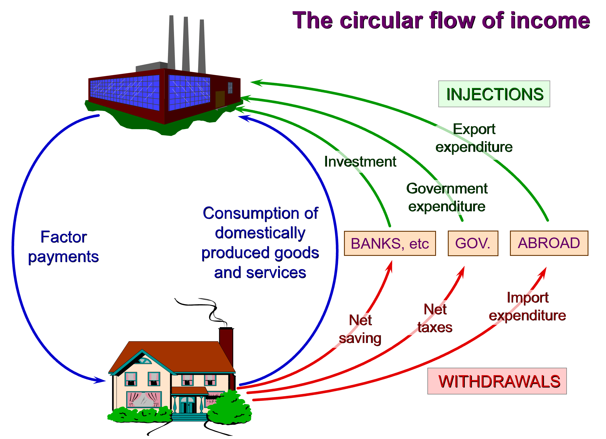 The fiscal stance is commonly estimated by measures of pubic-sector borrowing. To understand this, we can refer to the circular flow of income model. In this model, excesses of government spending (an injection) over taxation receipts (a withdrawal or leakage) represent a net injection into the circular flow and hence positively affect the level of aggregate demand for national output, all other things being equal.
A commonly used measure of borrowing in assessing the fiscal stance of the is the primary deficit. Unlike public-sector net borrowing, which is simply the excess of the sector’s spending over its receipts (largely taxation), the primary deficit subtracts net interest costs. It therefore excludes the interest payments on outstanding public-sector debts (and interest income earned on financial assets). The primary deficit can therefore be written as public-sector borrowing less net interest payments.
As discussed in our blog Fiscal impulses in November 2023, the primary deficit captures whether the public sector is able to afford its present fiscal choices by abstracting from debt-serving costs that reflect past fiscal choices. In this way, the primary deficit is a preferable measure to net borrowing both in assessing the impact on economic activity, i.e. the fiscal stance, and in assessing whether today’s fiscal choices will require government to issue additional debt.
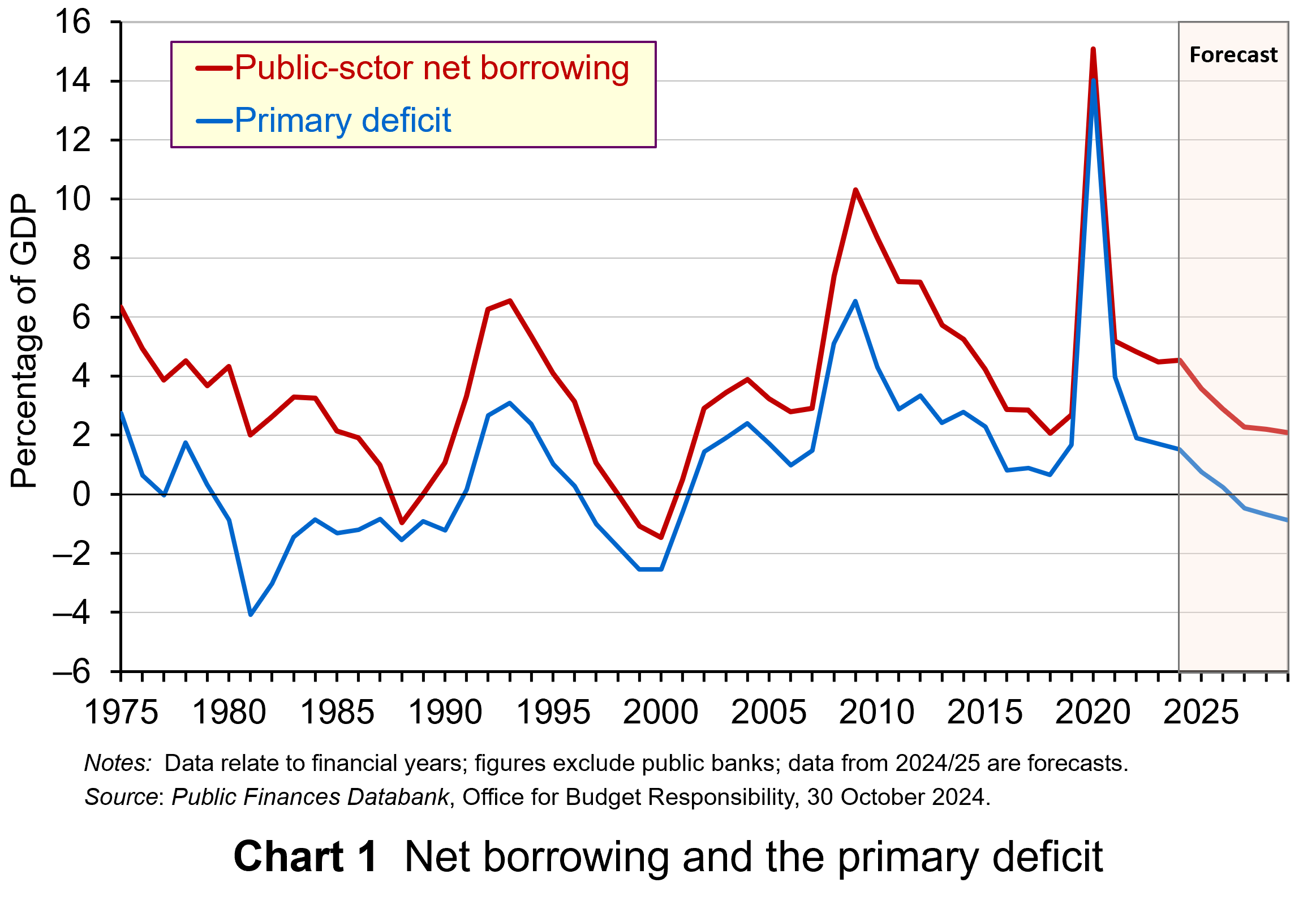 Chart 1 shows public-sector net borrowing and the primary balance as shares of GDP for the UK since financial year 1975/76 (click here for a PowerPoint). The data are from the latest Public Finances Databank published by the Office for Budget Responsibility, published on the day of the Autumn Budget in October (see Data links below).
Over the period 1975/6 to 2023/24, public-sector net borrowing and the primary deficit had averaged 3.8% and 1.3% of GDP respectively. In the financial year 2023/24, they were 4.5% and 1.5% (they had been as high as 15.1% and 14.1% in 2020/21 as a result of COVID support measures). In 2024/25 net borrowing and the primary deficit are forecast to be 4.5% and 1.6% respectively. By 2027/28, while net borrowing is forecast to be 2.3% of GDP, there is forecast to be a primary surplus of 0.7% of GDP.
The Autumn Budget lays out plans for higher tax revenues to contribute two-thirds of the overall reduction in the primary deficit over the forecast period (up to 2029/30), while spending decisions contribute the remaining third.
The largest tax-raising measure is an increase in the employer rate of National Insurance Contributions (NICs) by 1.2 percentage points to 15% from April 2025. This will be levied on employee wages above a Secondary Threshold of £5000, reduced from £9100, which will increase in line with CPI inflation each year from April 2028. (See John’s blog, Raising the minimum wage: its effects on poverty and employment, for an analysis on the effects of this change.) This measure, allowing for other changes to the operation of employer NICs, is expected to raise £122 billion over the forecast period. This amounts to over two-thirds of the additional tax take from the taxation measures taken in the Budget.
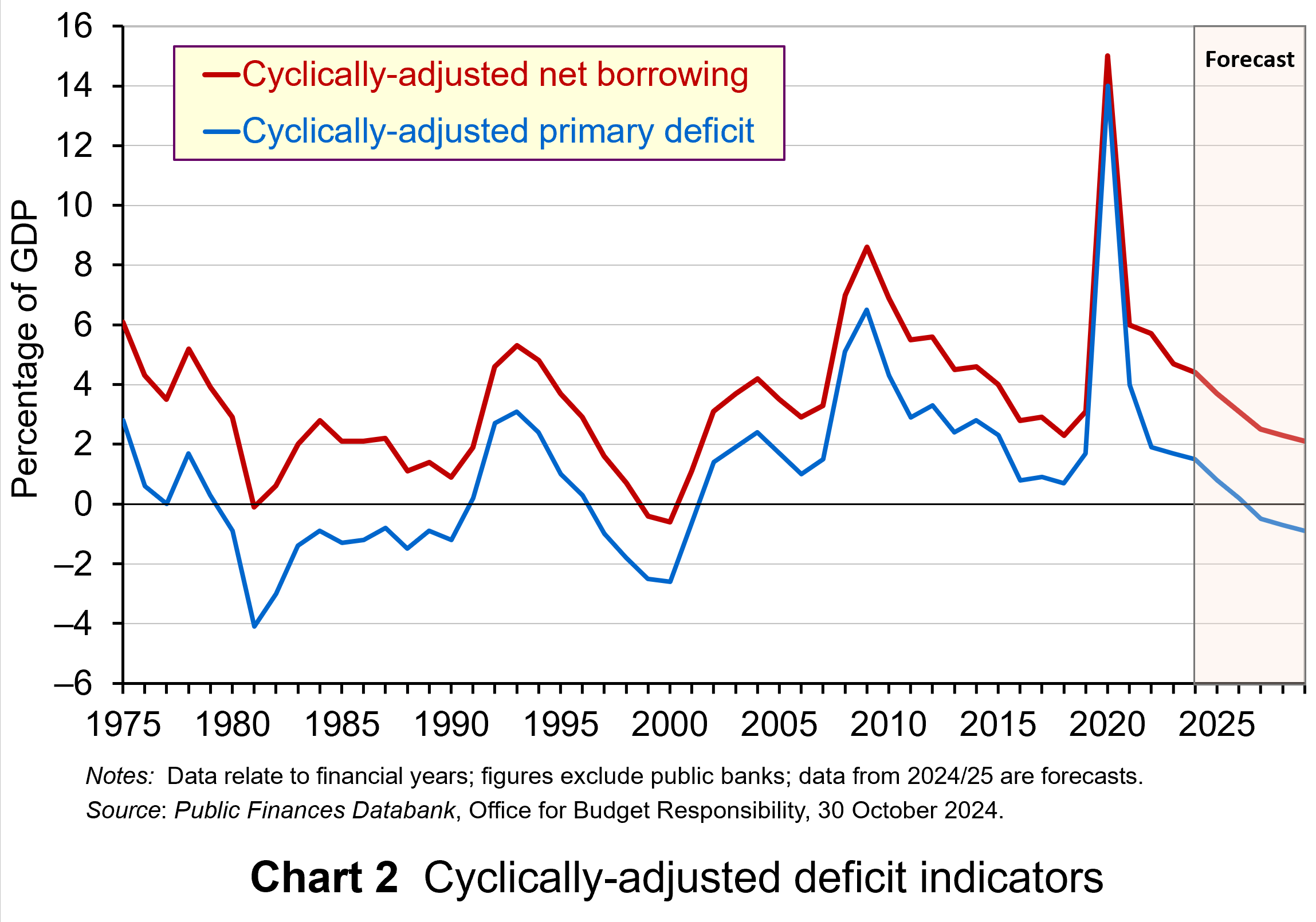 Chart 2 shows both net borrowing and the primary deficit after being cyclically-adjusted (click here for a PowerPoint). This process adjusts these fiscal indicators to account for those parts of spending and taxation that are affected by the position of the economy in the business cycle. These are those parts that act as automatic stabilisers helping, as the name suggests, to stabilise the economy.
The process of cyclical adjustment leads to estimates of receipts and expenditures as if the economy were operating at its potential output level and hence with no output gap. The act of cyclically adjusting the primary deficit, which is our preferred measure of the fiscal stance, allows us to assess better the public sector’s fiscal stance.
Over the period from 1975/6 up to and including 2023/24, the cyclically-adjusted primary deficit (CAPD) averaged 1.1% of GDP. In 2024/25 the CAPD is forecast to be 1.5% of GDP. It then moves to a surplus of 0.5% by 2027/28. It therefore mirrors the path of the unadjusted primary deficit.
Measuring the fiscal impulse
To assess even more clearly the extent to which the fiscal stance is changing, we can use the cyclically-adjusted primary deficit to measure a fiscal impulse. This captures the magnitude of change in discretionary fiscal policy.
The term should not be confused with fiscal multipliers which measure the impact of fiscal changes on outcomes, such as real GDP and employment. Instead, we are interested in the size of the impulse that the economy is being subject to. Specifically, we are measuring discretionary fiscal policy changes that result in structural changes in the government budget and which, therefore, allow an assessment of how much, if at all, a country’s fiscal stance has tightened or loosened.
The size of the fiscal impulse is measured by the year-on-year percentage point change in the cyclically-adjusted public-sector primary deficit (CAPD) as a percentage of GDP. A larger deficit or a smaller surplus indicates a fiscal loosening. This is consistent with a positive fiscal impulse. On the other hand, a smaller deficit or a larger surplus indicates a fiscal tightening. This is consistent with a negative fiscal impulse.
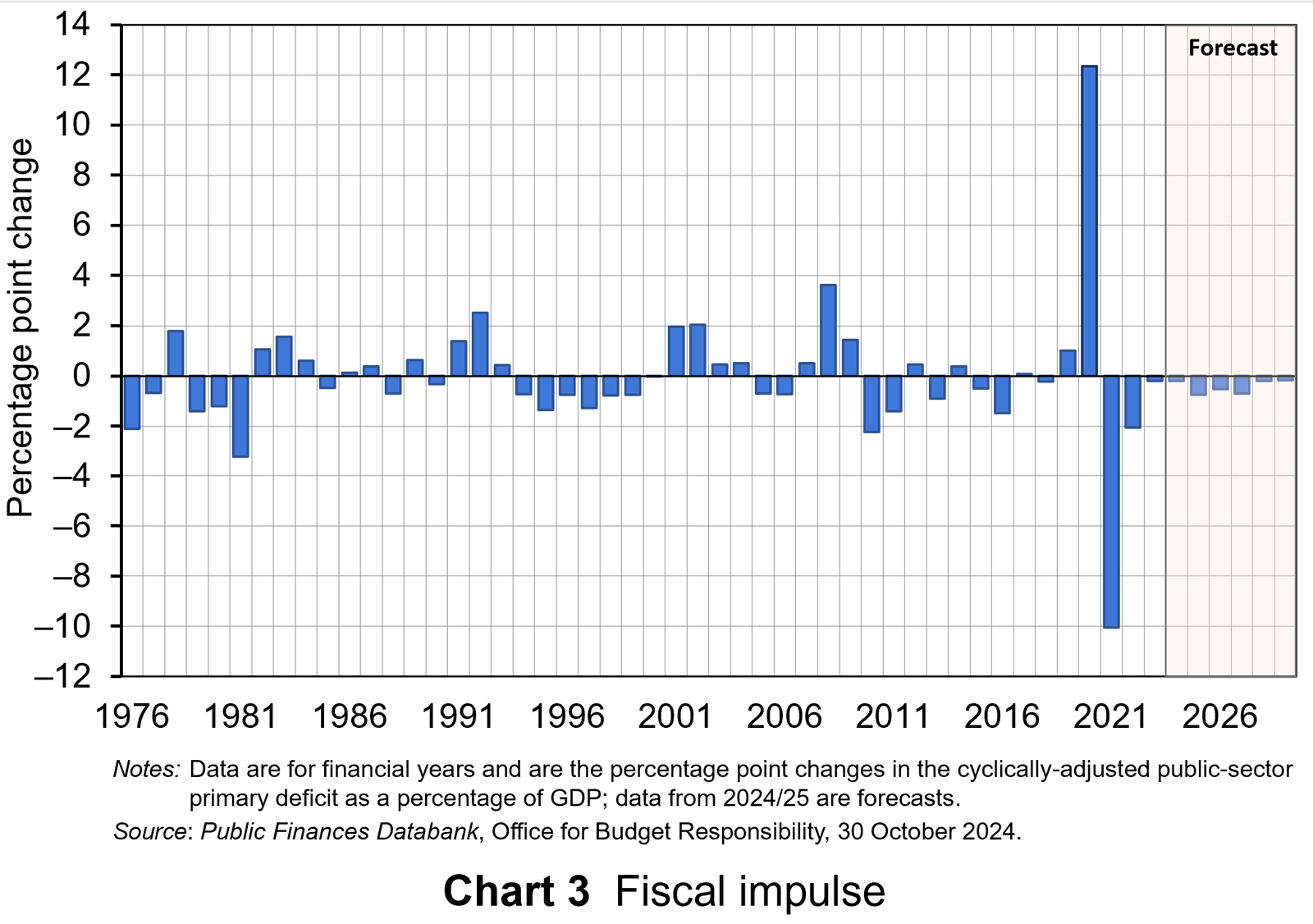 Chart 3 shows the magnitude of UK fiscal impulses since the mid-1970s (Click here for a PowerPoint file). The scale of the fiscal interventions in response to the COVID-19 pandemic, which included the COVID-19 Business Interruption Loan Scheme (CBILS) and Job Retention Scheme (‘furlough’), stand out sharply. In 2020 the CAPD to output ratio rose from 1.7 to 14.4%. This represents a positive fiscal impulse of 12.4% of GDP.
This was followed in 2021 by a tightening of the fiscal stance, with a negative fiscal impulse of 10.1% of GDP as the CAPD to output fell back to 4.0%. Subsequent tightening was tempered by policy measures to limit the impact on the private sector of the cost-of-living crisis, including the Energy Price Guarantee and Energy Bills Support Scheme.
For comparison, the fiscal response to the global financial crisis from 2007 to 2009 saw a cumulative positive fiscal impulse of 5.6% of GDP. While smaller in comparison to the discretionary fiscal responses to the COVID-19 pandemic, it nonetheless represented a sizeable loosening of the fiscal stance.
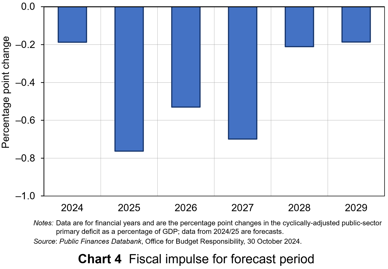 Chart 4 focuses on the implied fiscal impulse for the forecast period up to 2029/30 (click here for a PowerPoint). The period is notable for a negative fiscal impulse each year. Across the period as a whole, this there is a cumulative negative fiscal impulse of 2.6% of GDP. Most of the ‘heavy-lifting’ of the fiscal consolidation occurs in the three financial years from 2025/26 during which there is a cumulative negative impulse of 2.0% of GDP.
Looking forward
To conclude, we consider the implications for the projected profiles of public-sector spending, receipts and liabilities over the forecast period up to 2029/30.
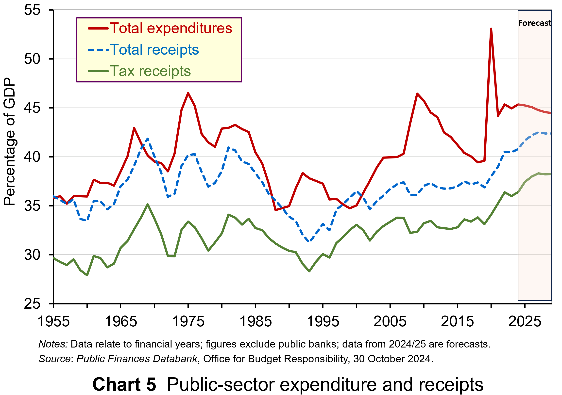 Chart 5 plots data since the mid-1950s (click here for a PowerPoint). It shows the size of total public-sector spending (also known as ‘total managed expenditures’), taxation receipts (sometimes referred as the ‘tax burden’) and total public-sector receipts as shares of GDP. This last one includes additional receipts, such as interest payments on financial assets and income generated by public corporations, as well as taxation receipts.
The OBR forecasts that in real terms (i.e. after adjustment for inflation), public-sector spending will increase on average over the period from 2025/26 to 2029/30 by 1.4% per year, but with total receipts due to rise more quickly at 2.5% per year and taxation receipts by 2.8% per year. The implications of this, as discussed in the OBR’s October 1014 Economic and Fiscal Outlook (see link below), are that:
the size of the state is forecast to settle at 44% of GDP by the end of the decade, almost 5 percentage points higher than before the pandemic” while additional tax revenues will “push the tax take to a historic high of 38% of GDP by 2029-30
Finally, the government has committed to two key rules: a stability rule and an investment rule.
The stability rule. This states that the current budget must be in surplus by 2029/30 or, once 2029/30 becomes the third year of the forecast period, it will be in balance or surplus every third year of the rolling forecast period thereafter. The current budget refers to the difference between receipts and expenditures other than capital expenditures. In effect, it captures the ability of government to meet day-to-day spending and is intended to ensure that over the medium term any borrowing is solely for investment. It is important to note that ‘balance’ is defined in a range of between a deficit and surplus of no more than 0.5% of GDP.
The stability rule replaces the borrowing rule of the previous government that public net borrowing, therefore inclusive of investment expenditures, was not to exceed 3% of GDP by the fifth year of the rolling forecast period.
 The investment rule. The government is planning to increase investment. In order to do this in a financially sustainable way, the investment rule states that public-sector net financial liabilities (PSNFL) or net financial debt for short, is falling as a share GDP by 2029/30, until 2029/30 becomes the third year of the forecast period. PSNFL should then fall by the third year of the rolling forecast period. PSNFL is a broader measure of the sector’s balance sheet than public-sector net debt (PSND), which was targeted under the previous government and which was required to fall by the fifth year of the rolling forecast period.
The new target, as well as now extending to the Bank of England, ‘nets off’ not just liquid assets (i.e. cash in the bank and foreign exchange reserves) but also financial assets such as shares and money owed to it, including expected student loan repayments. While liabilities are broader too, including for example, the local government pension scheme, the impact is expected to reduce the new liabilities target by £236 billion or 8.2 percentage points of GDP in 2024/25. The hope is that both rules can support what the Budget Report labels a ‘step change in investment’.
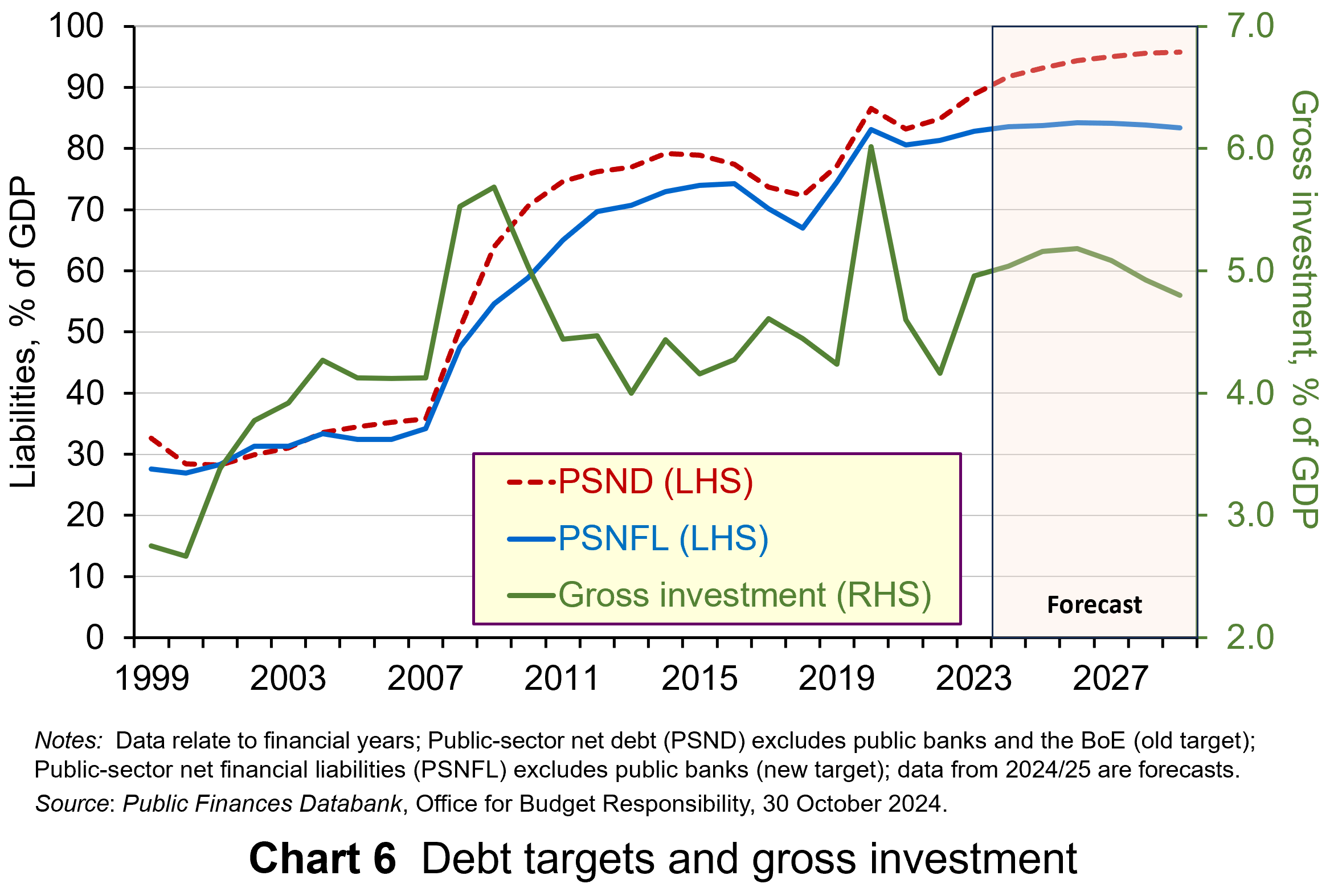 As Chart 6 shows, public investment as a share of GDP has not exceeded 6% this century and during the 2010s averaged only 4.4% (click here for a PowerPoint). The forecast has it rising above 5% for a time, but easing to 4.8% by end of the period.
This suggests more progress will be needed if the UK is to experience a significant and enduring increase in public investment. Of course, this needs to be set in the context of the wider public finances and is illustrative of the choices facing fiscal policymakers across the globe after the often violent shocks that have rocked economies and impacted on the state of the public finances in recent years.
Articles
Official documents
Data
Questions
- Explain what is meant by the following fiscal terms:
(a) Structural deficit,
(b) Automatic stabilisers,
(c) Discretionary fiscal policy,
(d) Public-sector net borrowing,
(e) Primary deficit,
(f) Current budget balance,
(g) Public-sector net financial liabilities (PSNFL).
- Explain the difference between a fiscal impulse and a fiscal multiplier.
- In designing fiscal rules what issues might policymakers need to consider?
- What are key differences between the fiscal rules of the previous Conservative government and the new Labour government in the UK? What economic arguments would you make for and against the ‘old’ and ‘new’ fiscal rules?
- What is meant by the ‘sustainability’ of the public finances? What factors might impact on their sustainability?
 The UK Chancellor of the Exchequer, Jeremy Hunt, delivered his Spring Budget on 6 March 2024. In his speech, he announced a cut in national insurance (NI): a tax paid by workers on employment or self-employment income. The main rate of NI for employed workers will be cut from 10% to 8% from 6 April 2024. This follows a cut this January from 12% to 10%. The rate for the self-employed will be cut from 9% to 6% from 6 April. These will be the new marginal rates from the NI-free threshold of £12 750 to the higher threshold of £50 270 (above which the marginal rate is 2% and remains unchanged). Unlike income tax, NI applies only to income from work (employment or self-employment) and does not include pension incomes, rent, interest and dividends.
The cuts will make all employed and self-employed people earning more than £12 750 better off than they would have been without them. For employees on average incomes of £35 000, the two cuts will be worth £900 per year.
But will people end up paying less direct tax (income tax and NI) overall than in previous years? The answer is no because of the issue of fiscal drag (see the blog, Inflation and fiscal drag). Fiscal drag refers to the dampening effect on aggregate demand when higher incomes lead to a higher proportion being paid in tax. It occurs when there is a faster growth in incomes than in tax thresholds. This means that (a) the tax-free allowance accounts for a smaller proportion of people’s incomes and (b) a higher proportion of many people’s incomes will be paid at the higher income tax rate. Fiscal drag is especially acute when thresholds are frozen, when inflation is rapid and when real incomes rise rapidly.
Tax thresholds have been frozen since 2021 and the government plans to keep them frozen until 2028. This is illustrated in the following table.

According to the Institute for Fiscal Studies, the net effect of fiscal drag means that for every £1 given back to employed and self-employed workers by the NI cuts, £1.30 will have been taken away as a result of freezing thresholds between 2021 and 2024. This will rise to £1.90 in 2027/28.
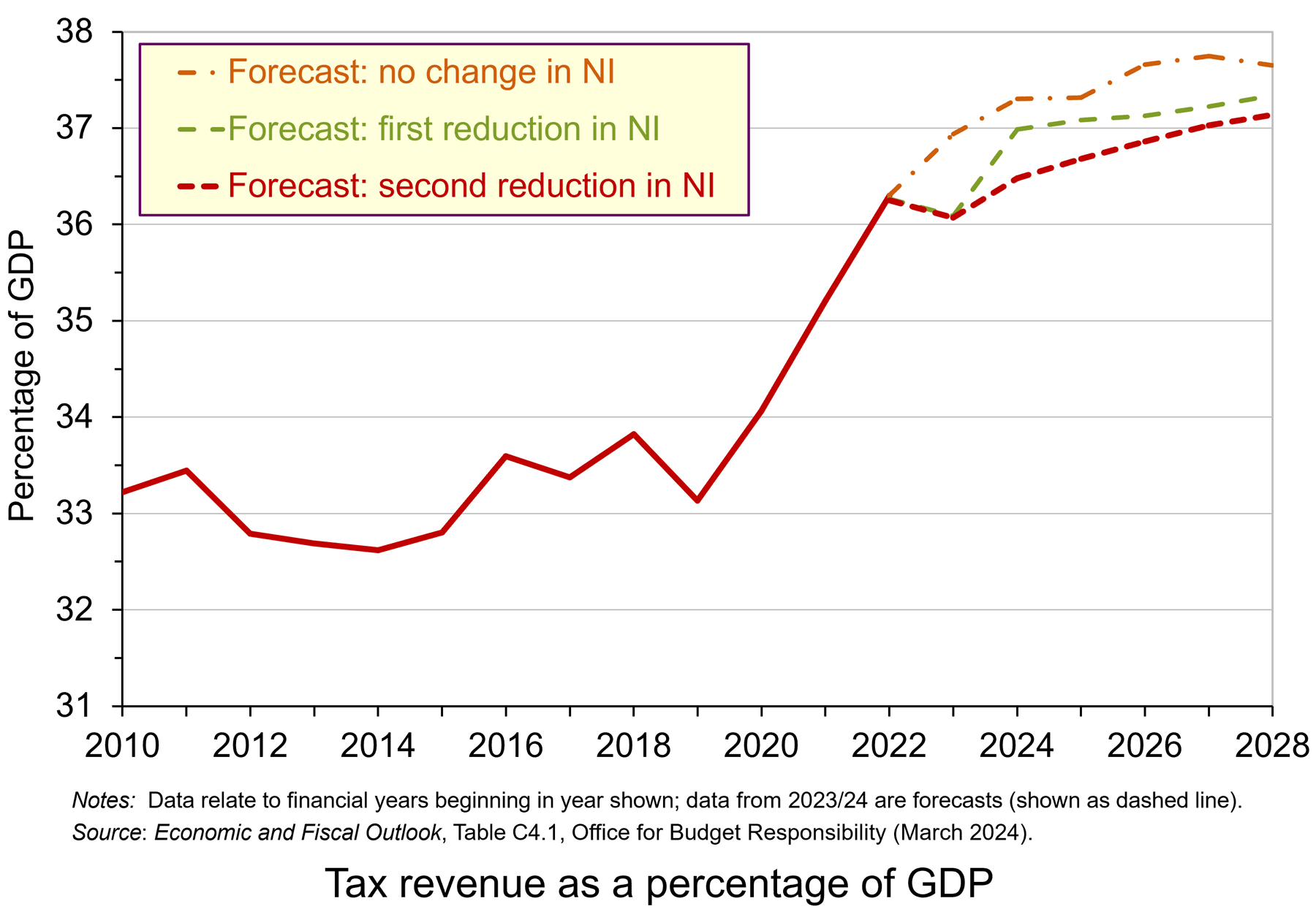 Tax revenues are still set to rise as a percentage of GDP. This is illustrated in the chart. Tax revenues were 33.2% of GDP in 2010/11. By 2022/23 the figure had risen to 36.3%. With neither of the two changes to NI (January 2024 and April 2024), the OBR forecasts that the figure would rise to 37.7% by 2028/29 – the top dashed line in the chart. After the first cut, announced in November, it forecasts a smaller rise to 37.3% – the middle dashed line. After the second cut, announced in the Spring Budget, the OBR cut the forecast figure to 37.1% – the bottom dashed line. (Click here for a PowerPoint of the chart.)
As you can see from the chart, despite the cut in NI rates, the fiscal drag from freezing thresholds means that tax revenue as a percentage of GDP is still set to rise.
Articles
Information, data and analysis
Questions
- Would fiscal drag occur with frozen nominal tax bands if there were zero real growth in incomes? Explain.
- Find out what happened to other taxes, benefits, reliefs and incentives in the 2024 Spring Budget. Assess their macroeconomic effect.
- If the government decides that it wishes to increase tax revenues as a proportion of GDP (for example, to fund increased government expenditure on infrastructure and socially desirable projects and benefits), examine the arguments for increasing personal allowances and tax bands in line with inflation but raising the rates of income tax in order to raise sufficient revenue?
- Distinguish between market-orientated and interventionist supply-side policies? Why do political parties differ in their approaches to supply-side policy?
- What is the Conservative government’s fiscal rule? Is the Spring Budget 2024 consistent with this rule?
- What policies were announced in the Spring Budget 2024 to increase productivity? Why is it difficult to estimate the financial outcome of such policies?
 The following blog is inspired by my teaching of macroeconomic issues to my final year students at Aston University. In the classes we’ve been discussing important aspects of monetary and fiscal policy design. What has become clear to me and my students is that the trade-offs which characterise the discipline of economics are certainly alive and well in the current environment in which monetary and fiscal policy choices are being made.
To demonstrate this we consider here some of the discussions we’ve had in class around central bank independence and monetary policy mandates. We’ve also looked at fiscal policy. Here we’ve examined the state of the public finances and the importance that seems to be attached to debt stabilisation and the imposition of debt rules.
Delegation and central bank mandates
My teaching this term began by introducing my students to one of the most important and influential monetary policy models. This is the model of Kydland and Prescott. Their model, published in the Journal of Political Economy in 1977 has become the theoretical bedrock for the modern-day operational independence of central banks.1
 The model explores how systemically high inflation can become established in economies when policymakers have the political incentive to lower unemployment or increase output above its long-run equilibrium value. This may be the case if governments operate monetary policy rather than the central bank (of if the central bank operates monetary policy but follows government objectives). By adopting expansionary monetary policy, governments can increase their popularity.
But this is likely to be short-lived, as any increased economic activity will only be temporary (assuming that the natural-rate hypothesis holds). Soon, inflation will rise.
But, if an election is on the horizon, there may be enough time to boost output and employment before inflation rises. In other words, an expectations-augmented Phillips curve may present governments with an incentive to loosen monetary policy and worry about the inflation consequences after the election.
However, the resulting ‘inflation surprise’ through the loosening of monetary policy means a fall in real pay and therefore in purchasing power. If people suspect that governments will be tempted to loosen policy, they will keep their expectations of inflation higher than the socially optimal inflation rate. Consequently, low-inflation targets lack credibility when governments have the temptation to loosen monetary policy. Such targets are time-inconsistent because governments have an incentive to renege and deliver higher inflation through a looser monetary policy. The result is an inflation bias.
Central bank independence
To prevent this inflationary bias arising, many central banks around the world have been given some form of operational independence with a mandate centred around an inflation-rate target. By delegating monetary policy to a more conservative central bank, the problem of inflationary bias can be addressed.
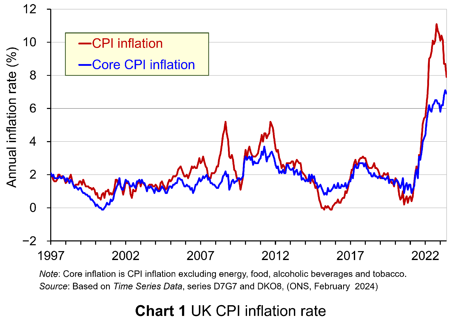 Yet central bank independence is not without its own issues and this has been an important part of the discussions with my students. Today, many economies are continuing to experience the effects of the inflationary shocks that began in 2021 (see Chart 1 for the UK CPI inflation rate: click here for a PowerPoint). The question is whether the appointment of a conservative or hard-nosed hawkish central banker trades off the stabilisation of inflation for greater volatility in output or unemployment.
The inflation–output stabilisation trade-off is closely associated with the works of Kenneth Rogoff2 and John Taylor3. The latter is known for his monetary policy rule, which has become known as the ‘Taylor rule’. This advocates that a rules-based central bank ought to place weight on both inflation and output stabilisation.
This is not without its own issues, however, since, by also placing weight on output stabilisation, we are again introducing the possibility of greater inflationary bias in policy making. Hence, while the act of delegation and a rules- or target-based approach may mitigate the extent of the bias relative to that in the Kydland and Prescott model, there nonetheless still remain issues around the design of the optimal framework for the conduct of monetary policy.
Indeed, the announcement that the UK had moved into recession in the last two quarters of 2023 can be seen as evidence that an otherwise abstract theoretical trade-off between inflation and output stabilisation is actually very real.
My classroom discussions have also shown how economic theory struggles to identify an optimal inflation-rate target. Beyond accepting that a low and stable inflation rate is desirable, it is difficult to address fully the student who asks what is so special about a 2% inflation target. Would not a 3% target, for example, be preferable, they might ask?
Whilst this may sound somewhat trivial, it has real-world consequences. In a world that now seems to be characterised by greater supply-side volatility and by more frequent inflation shocks than we were used to in recent history, might a higher inflation rate target be preferable? Certainly, one could argue that, with an inflation–output stabilisation trade-off, there is the possibility that monetary policy could be unduly restrictive in our potential new macroeconomic reality. Hence, we might come to see governments and central banks in the near future revisiting the mandates that frame the operation of their monetary policy. Time will tell.
Fiscal policy and debt stabilisation
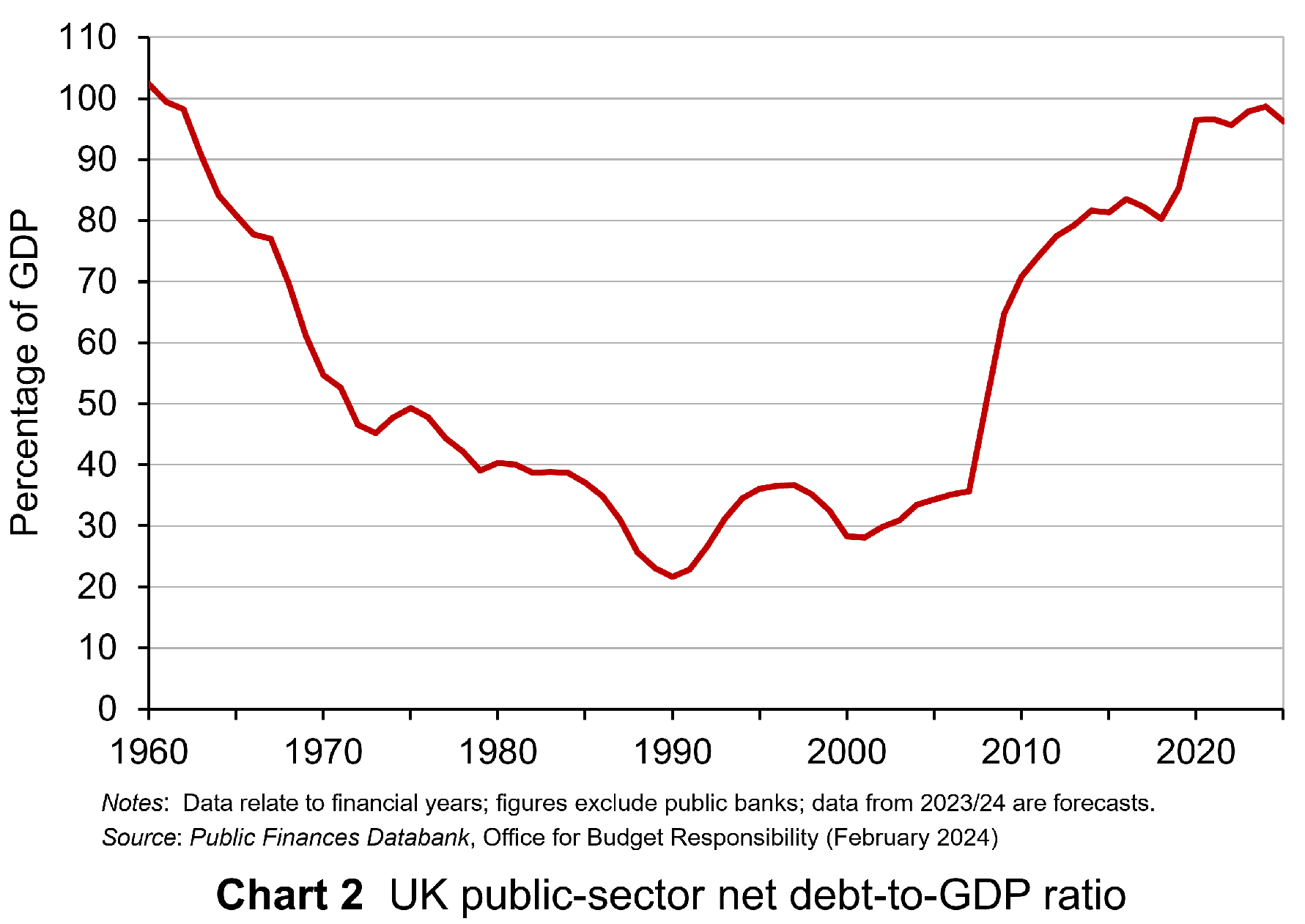 The second topic area that I have been discussing in my final-year macroeconomics classes has centred around fiscal policy and the state of the public finances. The context for this is that we have seen a significant increase in public debt-to-GDP ratios over the past couple of decades as the public sector has attempted to absorb significant economic shocks. These include the global financial crisis of 2007–8, the COVID-19 pandemic and the cost-of-living crisis. These interventions in the case of the UK have seen its public debt-to-GDP ratio more than triple since the early 2000s to close to 100% (see Chart 2: click here for a PowerPoint).
Understandably, given the stresses placed on the public finances, economists have increasingly debated issues around debt sustainability. These debates have been mirrored by politicians and policymakers. A key question is whether to have a public debt rule. The UK has in recent years adopted such a rule. The arguments for a rule centre on ensuring sound public finances and maintaining the confidence of investors to purchases public debt. A debt rule therefore places a discipline on fiscal policy, with implications for taxation and spending.
How easy it is to stick to a debt rule depends on three key factors. It will be harder to stick to the rule:
- The higher the current debt-to-GDP ratio and hence the more it needs to be reduced to meet the rule.
- The higher the rate of interest and hence the greater the cost of servicing the public debt.
- The lower the rate of economic growth and hence the less quickly will tax revenues rise.
With a given debt-to-GDP ratio, a given average interest rate payable on its debt, and a given rate of economic growth, we can determine the primary fiscal balance relative to GDP a government would need to meet for the debt-to-GDP ratio to remain stable. This is known as the ‘debt-stabilising primary balance’. The primary balance is the difference between a government’s receipts and its expenditures less the interest payments on its debt.
 This fiscal arithmetic is important in determining a government’s fiscal choices. It shows the implications for spending and taxation. These implications become ever more important and impactful on people, businesses, and society when the fiscal arithmetic becomes less favourable. This is a situation that appears to be increasingly the case for many countries, including the UK, as the rate of interest on public debt rises relative to a country’s rate of economic growth. As this happens, governments are increasingly required to run healthier primary balances. This of course implies a tightening of their fiscal stance.
Hence, the fiscal conversations with my students have focused on both the benefits and the costs of debt-stabilisation. In respect of the costs, a few issues have arisen.
First, as with the inflation-rate target, it is hard to identify an optimal public debt-to-GDP ratio number. While the fiscal arithmetic may offer some clue, it is not straightforward to address the question as to whether a debt-to-GDP ratio of say 100% or 120% would be excessive for the UK.
Second, it is possible that the debt stabilisation itself can make the fiscal arithmetic of debt stabilisation more difficult. This occurs if fiscal consolidation itself hinders long-term economic growth, which then makes the fiscal arithmetic more difficult. This again points to the difficulties in designing policy frameworks, whether they be for monetary or fiscal policy.
Third, a focus on debt stabilisation alone ignores the fact that there are two sides to any sector’s balance sheet. It would be very unusual when assessing the well-being of businesses or households if we were to ignore the asset side of their balance sheet. Yet, this is precisely the danger of focusing on public debt at the exclusion of what fiscal choices can mean for public-sector assets, from which we all can potentially benefit. Hence, some would suggest a more balanced approach to assessing the soundness of the public finances might involve a net worth (assets less liabilities) measure. This has parallels with the debates around whether mandates of central banks should be broader.
Applications in macroeconomics
What my teaching of a topics-based macroeconomics module this term has vividly demonstrated is that concepts, theories, and models come alive, and are capable of being understood better, when they are used to shine a light on real-world issues. The light being shone on monetary and fiscal policy in today’s turbulent macroeconomic environment is perhaps understandably very bright.
Indeed, the light being shone on fiscal policy in the UK and some other countries facing an upcoming election, is intensified further with the state of the public finances shaping much of the public discourse on fiscal choices. Hopefully, my students will continue to debate these important issues beyond their graduation, stressing their importance for people’s lives and, in doing so, going beyond the abstract.
References
- Rules rather than discretion: The inconsistency of optimal plans
The Journal of Political Economy, Finn E Kydland and Edward C. Prescott (1977, 85(3), pp 473–92)
- The optimal degree of commitment to an intermediate monetary target
Quarterly Journal of Economics, Kenneth Rogoff (November 1985, 100(4), pp 1169–89)
- Discretion versus policy rules in practice
Carnegie-Rochester Conference Series on Public Policy, John B Taylor (December 1993, 39, pp 195–214)
Articles
Questions
- What is meant by time-inconsistent monetary policy announcements? How has this concept been important for the way in which many central banks now conduct monetary policy?
- What is meant by a ‘conservative’ central banker? Why is the appointment of this type of central banker thought to be important in affecting inflation?
- What is the contemporary macroeconomic relevance of the inflation–output (or inflation–unemployment) stabilisation trade-off?
- How is the primary balance different from the actual budget balance?
- What do you understand by the concept of ‘the fiscal arithmetic’. Explain how each element of the fiscal arithmetic affects the debt-stabilising primary balance?
- Analyse the costs of benefits of a debt-based fiscal rule.
 The past decade or so has seen large-scale economic turbulence. As we saw in the blog Fiscal impulses, governments have responded with large fiscal interventions. The COVID-19 pandemic, for example, led to a positive fiscal impulse in the UK in 2020, as measured by the change in the structural primary balance, of over 12 per cent of national income.
The scale of these interventions has led to a significant increase in the public-sector debt-to-GDP ratio in many countries. The recent interest rates hikes arising from central banks responding to inflationary pressures have put additional pressure on the financial well-being of governments, not least on the financing of their debt. Here we discuss these pressures in the context of the ‘r – g’ rule of sustainable public debt.
Public-sector debt and borrowing
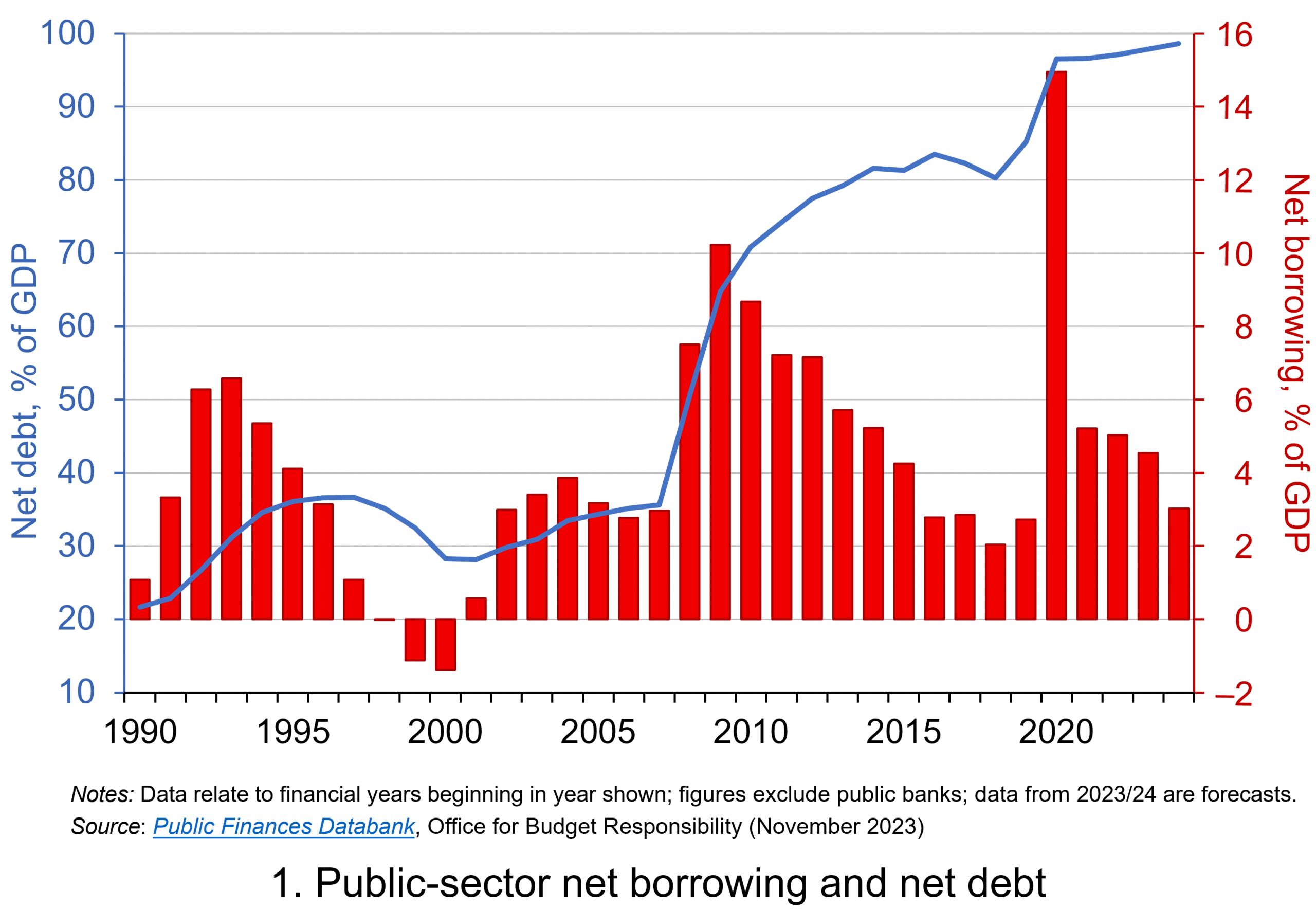 Chart 1 shows the path of UK public-sector net debt and net borrowing, as percentages of GDP, since 1990. Debt is a stock concept and is the result of accumulated flows of past borrowing. Net debt is simply gross debt less liquid financial assets, which mainly consist of foreign exchange reserves and cash deposits. Net borrowing is the headline measure of the sector’s deficit and is based on when expenditures and receipts (largely taxation) are recorded rather than when cash is actually paid or received. (Click here for a PowerPoint of Chart 1)
Chart 1 shows the impact of the fiscal interventions associated with the global financial crisis and the COVID-19 pandemic, when net borrowing rose to 10 per cent and 15 per cent of GDP respectively. The former contributed to the debt-to-GDP ratio rising from 35.6 per cent in 2007/8 to 81.6 per cent in 2014/15, while the pandemic and subsequent cost-of-living interventions contributed to the ratio rising from 85.2 per cent in 2019/20 to around 98 per cent in 2023/24.
Sustainability of the public finances
 The ratcheting up of debt levels affects debt servicing costs and hence the budgetary position of government. Yet the recent increases in interest rates also raise the costs faced by governments in financing future deficits or refinancing existing debts that are due to mature. In addition, a continuation of the low economic growth that has beset the UK economy since the global financial crisis also has implications for the burden imposed on the public sector by its debts, and hence the sustainability of the public finances. After all, low growth has implications for spending commitments, and, of course, the flow of receipts.
The analysis therefore implies that the sustainability of public-sector debt is dependent on at least three factors: existing debt levels, the implied average interest rate facing the public sector on its debts, and the rate of economic growth. These three factors turn out to underpin a well-known rule relating to the fiscal arithmetic of public-sector debt. The rule is sometimes known as the ‘r – g’ rule (i.e. the interest rate minus the growth rate).
Underpinning the fiscal arithmetic that determines the path of public-sector debt is the concept of the ‘primary balance’. This is the difference between the sector’s receipts and its expenditures less its debt interest payments. A primary surplus (a positive primary balance) means that receipts exceed expenditures less debt interest payments, whereas a primary deficit (a negative primary balance) means that receipts fall short. The fiscal arithmetic necessary to prevent the debt-to-GDP ratio rising produces the following stable debt equation or ‘r – g’ rule:
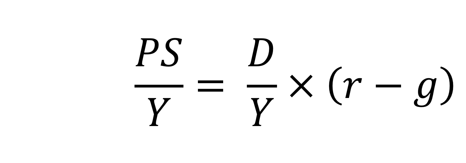
On the left-hand side of the stable debt equation is the required primary surplus (PS) to GDP (Y) ratio. Moving to the right-hand side, the first term is the existing debt-to-GDP ratio (D/Y). The second term ‘r – g’, is the differential between the average implied interest rate the government pays on its debt and the growth rate of the economy. These terms can be expressed in either nominal or real terms as this does not affect the differential.
To illustrate the rule consider a country whose existing debt-to-GDP ratio is 1 (i.e. 100 per cent) and the ‘r – g’ differential is 0.02 (2 percentage points). In this scenario they would need to run a primary surplus to GDP ratio of 0.02 (i.e. 2 percent of GDP).
The ‘r – g‘ differential
The ‘r – g’ differential reflects macroeconomic and financial conditions. The fiscal arithmetic shows that these are important for the dynamics of public-sector debt. The fiscal arithmetic is straightforward when r = g as any primary deficit will cause the debt-to-GDP ratio to rise, while a primary surplus will cause the ratio to fall. The larger is g relative to r the more favourable are the conditions for the path of debt. Importantly, if the differential is negative (r < g), it is possible for the public sector to run a primary deficit, up to the amount that the stable debt equation permits.
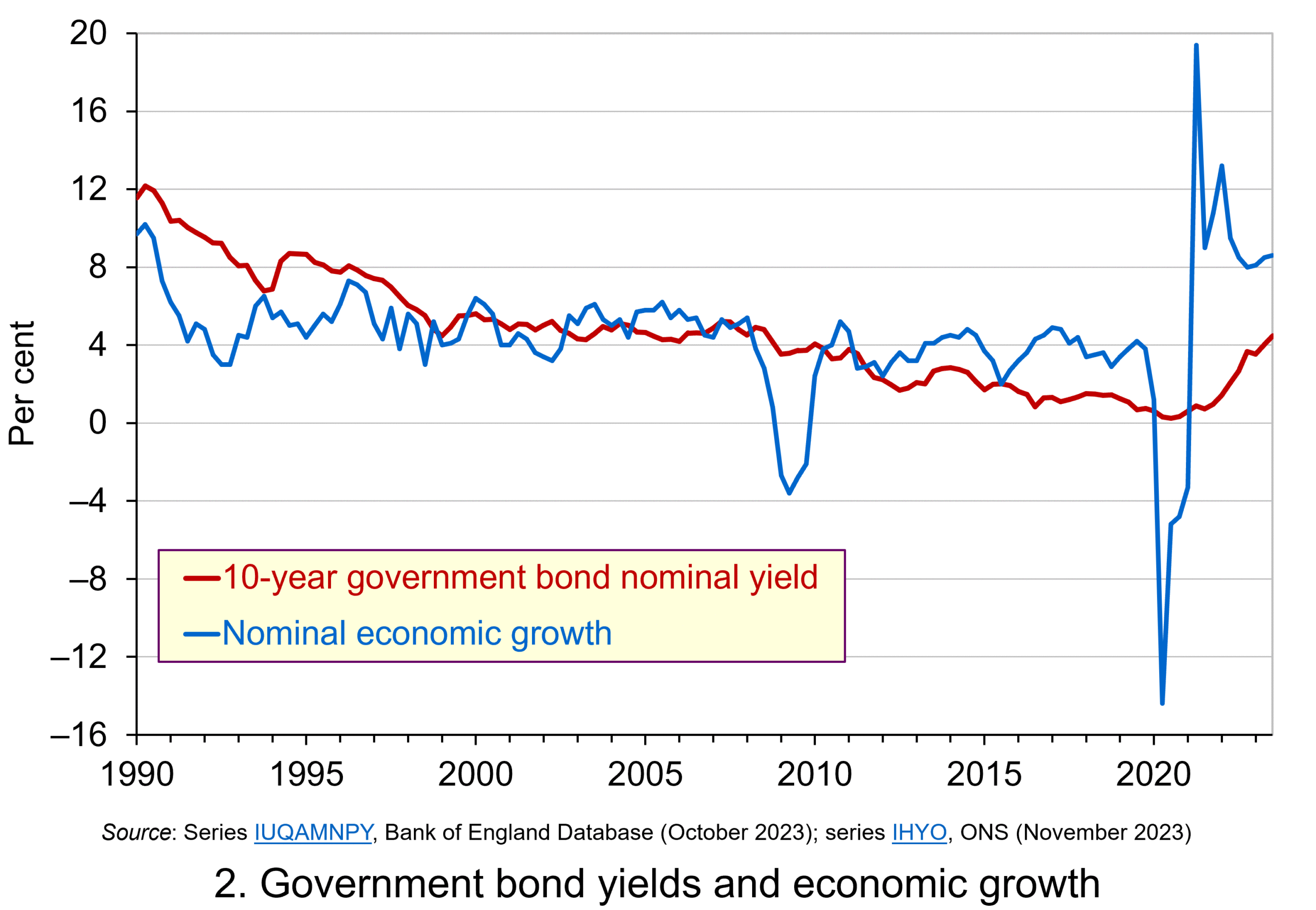 Consider Charts 2 and 3 to understand how the ‘r – g’ differential has affected debt sustainability in the UK since 1990. Chart 2 plots the implied yield on 10-year government bonds, alongside the annual rate of nominal growth (click here for a PowerPoint). As John explains in his blog The bond roller coaster, the yield is calculated as the coupon rate that would have to be paid for the market price of a bond to equal its face value. Over the period, the average annual nominal growth rate was 4.5 per cent, while the implied interest rate was almost identical at 4.6 per cent. The average annual rate of CPI inflation over this period was 2.8 per cent.
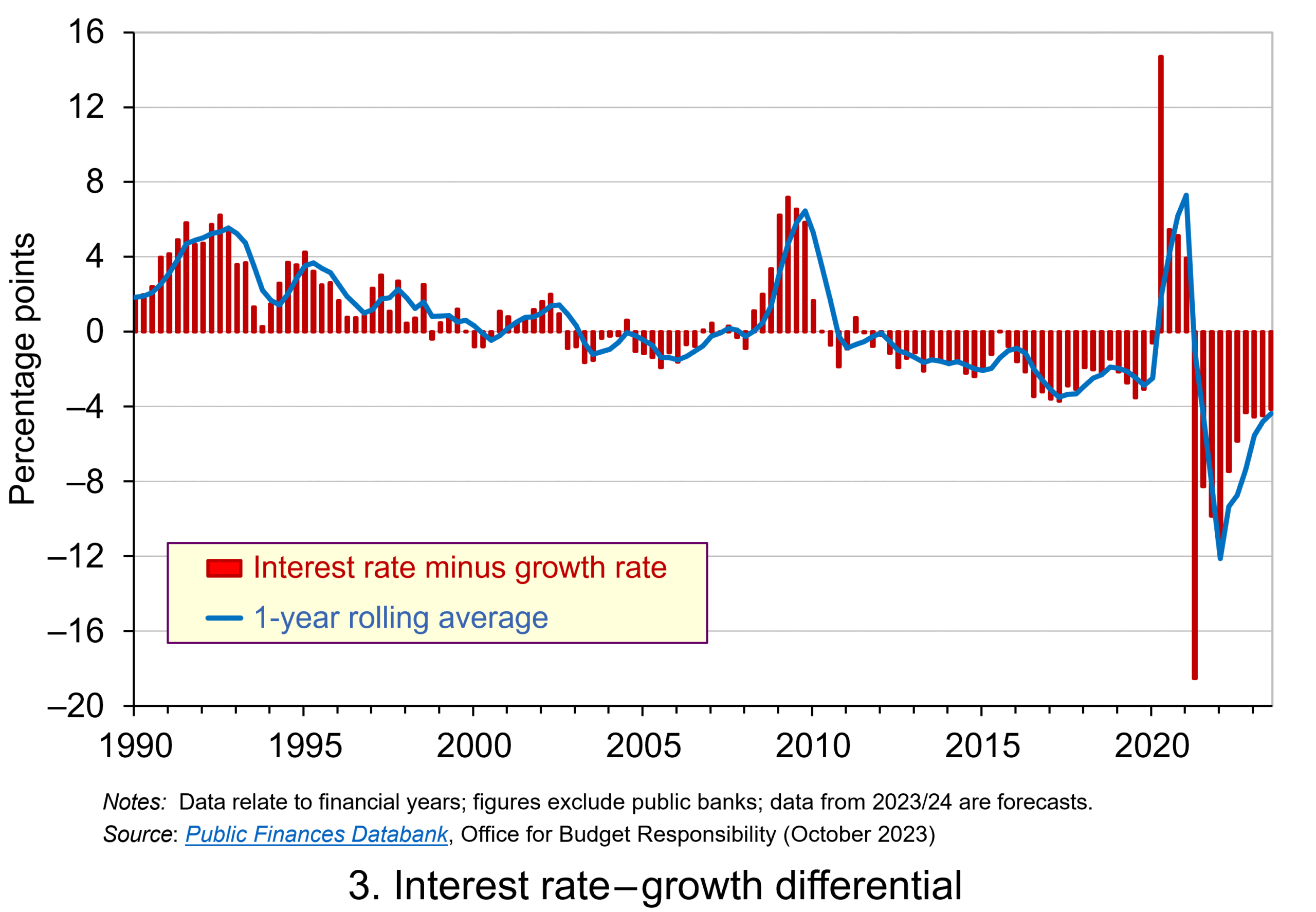 Chart 3 plots the ‘r – g’ differential which is simply the difference between the two series in Chart 2, along with a 12-month rolling average of the differential to help show better the direction of the differential by smoothing out some of the short-term volatility (click here for a PowerPoint). The differential across the period is a mere 0.1 percentage points implying that macroeconomic and financial conditions have typically been neutral in supporting debt sustainability. However, this does mask some significant changes across the period.
We observe a general downward trend in the ‘r – g’ differential from 1990 up to the time of the global financial crisis. Indeed between 2003 and 2007 we observe a favourable negative differential which helps to support the sustainability of public debt and therefore the well-being of the public finances. This downward trend of the ‘r – g’ differential was interrupted by the financial crisis, driven by a significant contraction in economic activity. This led to a positive spike in the differential of over 7 percentage points.
 Yet the negative differential resumed in 2010 and continued up to the pandemic. Again, this is indicative of the macroeconomic and financial environments being supportive of the public finances. It was, however, largely driven by low interest rates rather than by economic growth.
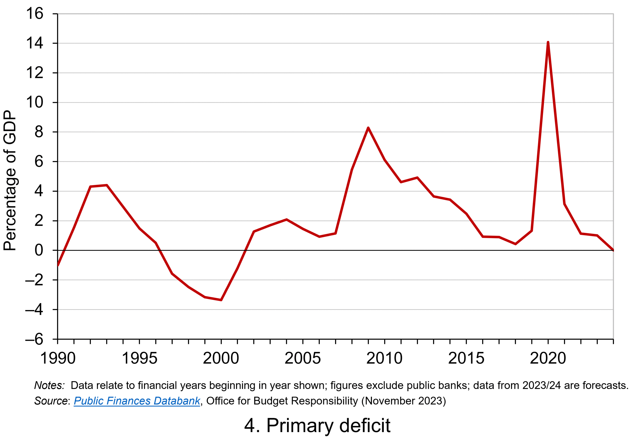
Consequently, the negative ‘r – g’ differential meant that the public sector could continue to run primary deficits during the 2010s, despite the now much higher debt-to-GDP ratio. Yet, weak growth was placing limits on this. Chart 4 indeed shows that primary deficits fell across the decade (click here for a PowerPoint).
The pandemic and beyond
 The pandemic saw the ‘r – g’ differential again turn markedly positive, averaging 7 percentage points in the four quarters from Q2 of 2020. While the differential again turned negative, the debt-to-GDP ratio had also increased substantially because of large-scale fiscal interventions. This made the negative differential even more important for the sustainability of the public finances. The question is how long the negative differential can last.
Looking forward, the fiscal arithmetic is indeed uncertain and worryingly is likely to be less favourable. Interest rates have risen and, although inflationary pressures may be easing somewhat, interest rates are likely to remain much higher than during the past decade. Geopolitical tensions and global fragmentation pose future inflationary concerns and a further drag on growth.
As well as the short-term concerns over growth, there remain long-standing issues of low productivity which must be tackled if the growth of the UK economy’s potential output is to be raised. These concerns all point to the important ‘r – g’ differential become increasingly less negative, if not positive. If so the fiscal arithmetic could mean increasingly hard maths for policymakers.
Articles
- The budget deficit: a short guide
House of Commons Library (8/6/23)
- If markets are right about long real rates, public debt ratios will increase for some time. We must make sure that they do not explode.
Peterson Institute for International Economics, Olivier Blanchard (6/11/23)
- The UK government’s debt nightmare
ITV News, Robert Peston (13/7/23)
- National debt could hit 300% of GDP by 2070s, independent watchdog the OBR warns
Sky News, James Sillars (13/7/23)
- How much money is the UK government borrowing, and does it matter?
BBC News (20/10/23)
- Cost of national debt hits 20-year high
BBC News, Vishala Sri-Pathma & Faisal Islam (4/10/23)
- Bond markets could see ‘mini boom-bust cycles’ as global government debt to soar by $5 trillion a yea
Markets Insider, Filip De Mott (16/11/23)
- The counterintuitive truth about deficits for bond investors
Financial Times, Matt King (17/11/23)
- UK government borrowing almost £20bn lower than expected
The Guardian, Richard Partington (20/10/23)
- Controlling debt is just a means — it is not a government’s end
Financial Times, Martin Wolf (13/11/23)
Data
Questions
- What is meant by each of the following terms: (a) net borrowing; (b) primary deficit; (c) net debt?
- Explain how the following affect the path of the public-sector debt-to-GDP ratio: (a) interest rates; (b) economic growth; (c) the existing debt-to-GDP ratio.
- Which factors during the 2010s were affecting the fiscal arithmetic of public debt positively, and which negatively?
- Discuss the prospects for the fiscal arithmetic of public debt in the coming years.
- Assume that a country has an existing public-sector debt-to-GDP ratio of 60 percent.
(a) Using the ‘rule of thumb’ for public debt dynamics, calculate the approximate primary balance it would need to run in the coming year if the expected average real interest rate on the debt were 3 per cent and real economic growth were 2 per cent?
(b) Repeat (a) but now assume that real economic growth is expected to be 4 per cent.
(c) Repeat (a) but now assume that the existing public-sector debt-to-GDP ratio is 120 per cent.
(d) Using your results from (a) to (c) discuss the factors that affect the fiscal arithmetic of the growth of public-sector debt.
 During the pandemic, millions of people’s wages in the UK were paid by the government to prevent the closure of businesses and a surge in unemployment. The furlough scheme officially came to an end in September 2021. However, with the spread of the Omicron variant and the fear of further restrictions being put in place, there has been a call by many to re-introduce the furlough scheme.
The furlough scheme
The furlough scheme began when the government brought in, what was officially called the Coronavirus Job Retention Scheme (CJRS) in early 2020. This was when the pandemic first forced businesses across the country to close. The scheme worked by paying part of employees’ wages, preventing the need for businesses to make their staff redundant, therefore avoiding a rapid rise in unemployment along with the associated costs. It also avoided the financial and emotional costs of firing and then rehiring workers post pandemic. Under the scheme, furloughed workers received 80% of their wages, up to £2500 a month, if they couldn’t work because of the impact of coronavirus. Employees were able to maintain the security of employment and the payments helped furloughed workers pay their bills.
 The scheme saw billions of pounds spent paying the wages of employees whose firms were forced to close temporarily. It could be argued that the expense of the scheme was a huge disadvantage. However, the alternative would have been for the government to pay unemployment-related benefits. Despite the furlough scheme being deemed necessary, it was not without its drawbacks for the structure of businesses. Rather than businesses adapting to changes in the economy and consumer demands, they could decide to claim the money and avoid the need to restructure. There was also concern about the length of the furlough scheme and the ability of businesses to bounce back post-pandemic.
Since the start of the scheme, the specifics of what was paid and who received it changed over time, especially once the economy started opening again. Initial steps were made to allow part-time return to work and the scheme started to wind down over the summer of 2021, with the government covering less of the wages and businesses covering more. From July, employers had to provide 10% of the wages of their furloughed staff, with the government paying the rest. This then increased to 20% in August with the CJRS coming to a complete end on 30 September 2021. At this point, there were around 1.6 million employees still receiving payment from the scheme.
Impact on Employment
With the end to the furlough scheme in September 2021, there were concerns that this would lead to a large number of redundancies. However, data indicate that has not happened and there is a record number of job vacancies. Official figures show that UK employment rose in October, confirming the strength of the labour market. The Office for National Statistics stated that the employment rate rose to 75.5% in the three months to October, up 0.2 percentage points on the previous quarter. This is believed to be driven by a rise in part-time work, which had dropped sharply during the pandemic. However, it is important to note that the strength in these numbers was prior to the emergence of the Omicron variant.
Omicron
 In November, the government had ruled out once again bankrolling people’s wages at enormous expense. However, the Chancellor is now under pressure to respond to the latest announcements around the ever-changing landscape of the pandemic. The fast-spreading mutation of the Covid-19 virus, Omicron, is posing a fresh threat to the economy.
On the 8 December, the Prime Minister announced new ‘Plan B’ Covid rules for England. As part of these new rules to limit the spread of Omicron, people are being asked to work from home again if possible and face masks are compulsory in most public places. Covid passes or a negative Covid test result are also needed to get into nightclubs and large venues.
Scotland and Wales have brought in further restrictions. Scotland’s First Minister, Nicola Sturgeon, has asked people to limit socialising to three households at a time in the run-up to Christmas. Shops and hospitality venues in Scotland must bring back physical distancing and screens. In Wales, nightclubs will close after 26 December and social distancing will be reintroduced in shops.
 Although the hospitality industry and retail sector remain open, they are facing a slump in trade thanks to the new restrictions and worries among the general public. With the work-from-home guidance and advice from health officials that people should limit their social interactions, pubs and restaurants have seen widespread cancellations in the run-up to Christmas. Trade is suffering and these mass cancellations come at a time when these sectors were hoping for bumper trade after a dismal last couple of years.
In light of these concerns, ministers are now being urged to guarantee support in case businesses have to shut. Despite the indication that it would be highly unlikely that the UK would experience a full return to the restrictions seen at previous stages of the crisis, the International Monetary Fund has stated that the UK government should be drawing up contingency plans. The IMF has called for a mini-furlough scheme in the event that the Omicron variant forces the government to close parts of the economy. The idea is that the mini-furlough scheme would see a limited version of the multi-billion-pound job subsidy scheme being rolled out if firms are forced to close.
There are strong calls for there to be targeted support, which this mini-furlough scheme could offer. The Resolution Foundation argued in mid-December that a furlough scheme tied solely to the hospitality industry would help prevent job loses in an industry that is currently suffering once again. It calculated that the cost of a hospitality-only furlough scheme would be £1.4 billion a month if it were pitched at the original level of 80% of wage support. If a January to March sector-specific scheme were to be introduced it is estimated to cost around £5 billion, a small cost in comparison to £46 billion spent on furlough so far.
Inflation
Any reintroduction of a furlough scheme would be a jolt for the government. This would mean a return to the 2020-style arguments around protecting livelihoods and businesses, a contrast to the recent messaging from the Treasury of restoring public finances. There is also concern about how this will all impact on current growth predictions and inflation concerns. The IMF expects the growth of the UK economy to be 6.8% in 2021 and 5% in 2022. However, the drawback from this is that the recovery would also be accompanied by rising inflation. It has been suggested, therefore, that interest rate increases from the Bank of England would be needed to keep inflation under control, while at the same time being not so great as to kill off growth.
It was widely expected that the Bank of England would again put off a rate hike in order to wait to see the economic impact of Plan B restrictions. However, on Thursday 16 December, interest rates were raised for the first time in more than three years. Despite the fears that Omicron could slow the economy by causing people to spend less, Bank Rate was raised from 0.1% to 0.25% . This came in the wake of data showing prices climbing at the fastest pace for 10 years.
Next Steps?
Government finances would take another huge hit if the furlough scheme were revived. But a version of such a scheme is likely to be necessary to avert an unemployment crisis and the attendant costs.
However, in resisting further measures, the government has argued that it has already acted early to help control the virus’s spread by rapidly rolling out booster jabs, while avoiding unduly damaging economic and social restrictions.
The government also argues that some of the measures from the total £400 billion Covid support package since the start of the pandemic will continue to help businesses into Spring 2022. Such measures include government-backed loans for small- and medium-sized businesses until June 2022, a reduction in VAT from 20% to 12.5% until March 2022 and business rates relief for eligible retail, hospitality, and leisure businesses until March 2022. Talks are ongoing with hospitality and and other business organisations directly affected by Covid restrictions.
The British Chambers of Commerce has argued that current measures are not enough and has called for VAT on hospitality and tourism to be cut back to its emergency rate of 5% and for the 100% business rates relief for retailers to return. The CBI has also called for any unspent local authority grants to be spent now to help affected firms and that further help, including business rates relief, should be on the table if restrictions continue after the government’s 5 January review date. The IMF said that with strong policy support, the economy had proved resilient, but it stressed that a return of some of the measures that prevented mass unemployment and large-scale business failures might soon be needed.
Conclusion
Infections caused by the new Omicron variant are rising rapidly, doubling every two to three days. It is expected to become the dominant variant in the UK soon with health officials warning it may be the most significant threat since the start of the pandemic. However, it is not yet known what the full extent of the impact of this new variant on the NHS will be, leaving the severity of future restrictions uncertain.
But what is evident is that the course of the pandemic has changed and there is a growing case for the government to start planning for new support packages. Although a reintroduction of the furlough scheme was hoped not to be needed on the path out of the pandemic, a short detour may be required in the form of a mini-furlough scheme. The size and reach of any support put in place will depend upon any further restrictions on economic activity.
Articles
Questions
- Should the level of support for business return to the levels in place earlier in 2021?
- What measures could a government put in place to curtail the spread of the Omicron variant that have only a minimal impact on business and employment?
- Compare the UK measures to curtail the spread of the virus with those used in some other European countries.
- What are the arguments for and against (a) re-introducing the furlough scheme as it was earlier in 2021; (b) introducing a version restricted to the hospitality sector?
 In this blog we show how we can apply fiscal metrics to assess the UK government’s fiscal stance. This captures the extent to which fiscal policy contributes to the level of economic activity in the economy.
 The fiscal stance is commonly estimated by measures of pubic-sector borrowing. To understand this, we can refer to the circular flow of income model. In this model, excesses of government spending (an injection) over taxation receipts (a withdrawal or leakage) represent a net injection into the circular flow and hence positively affect the level of aggregate demand for national output, all other things being equal.
  Chart 1 shows public-sector net borrowing and the primary balance as shares of GDP for the UK since financial year 1975/76 (click here for a PowerPoint). The data are from the latest Public Finances Databank published by the Office for Budget Responsibility, published on the day of the Autumn Budget in October (see Data links below).
 Chart 2 shows both net borrowing and the primary deficit after being cyclically-adjusted (click here for a PowerPoint). This process adjusts these fiscal indicators to account for those parts of spending and taxation that are affected by the position of the economy in the business cycle. These are those parts that act as automatic stabilisers helping, as the name suggests, to stabilise the economy.
 Chart 3 shows the magnitude of UK fiscal impulses since the mid-1970s (Click here for a PowerPoint file). The scale of the fiscal interventions in response to the COVID-19 pandemic, which included the COVID-19 Business Interruption Loan Scheme (CBILS) and Job Retention Scheme (‘furlough’), stand out sharply. In 2020 the CAPD to output ratio rose from 1.7 to 14.4%. This represents a positive fiscal impulse of 12.4% of GDP.
 Chart 4 focuses on the implied fiscal impulse for the forecast period up to 2029/30 (click here for a PowerPoint). The period is notable for a negative fiscal impulse each year. Across the period as a whole, this there is a cumulative negative fiscal impulse of 2.6% of GDP. Most of the ‘heavy-lifting’ of the fiscal consolidation occurs in the three financial years from 2025/26 during which there is a cumulative negative impulse of 2.0% of GDP.
 Chart 5 plots data since the mid-1950s (click here for a PowerPoint). It shows the size of total public-sector spending (also known as ‘total managed expenditures’), taxation receipts (sometimes referred as the ‘tax burden’) and total public-sector receipts as shares of GDP. This last one includes additional receipts, such as interest payments on financial assets and income generated by public corporations, as well as taxation receipts.
 The investment rule. The government is planning to increase investment. In order to do this in a financially sustainable way, the investment rule states that public-sector net financial liabilities (PSNFL) or net financial debt for short, is falling as a share GDP by 2029/30, until 2029/30 becomes the third year of the forecast period. PSNFL should then fall by the third year of the rolling forecast period. PSNFL is a broader measure of the sector’s balance sheet than public-sector net debt (PSND), which was targeted under the previous government and which was required to fall by the fifth year of the rolling forecast period.
  As Chart 6 shows, public investment as a share of GDP has not exceeded 6% this century and during the 2010s averaged only 4.4% (click here for a PowerPoint). The forecast has it rising above 5% for a time, but easing to 4.8% by end of the period.
 Tax revenues are still set to rise as a percentage of GDP. This is illustrated in the chart. Tax revenues were 33.2% of GDP in 2010/11. By 2022/23 the figure had risen to 36.3%. With neither of the two changes to NI (January 2024 and April 2024), the OBR forecasts that the figure would rise to 37.7% by 2028/29 – the top dashed line in the chart. After the first cut, announced in November, it forecasts a smaller rise to 37.3% – the middle dashed line. After the second cut, announced in the Spring Budget, the OBR cut the forecast figure to 37.1% – the bottom dashed line. (Click
  The following blog is inspired by my teaching of macroeconomic issues to my final year students at Aston University. In the classes we’ve been discussing important aspects of monetary and fiscal policy design. What has become clear to me and my students is that the trade-offs which characterise the discipline of economics are certainly alive and well in the current environment in which monetary and fiscal policy choices are being made.
 The model explores how systemically high inflation can become established in economies when policymakers have the political incentive to lower unemployment or increase output above its long-run equilibrium value. This may be the case if governments operate monetary policy rather than the central bank (of if the central bank operates monetary policy but follows government objectives). By adopting expansionary monetary policy, governments can increase their popularity.
 Yet central bank independence is not without its own issues and this has been an important part of the discussions with my students. Today, many economies are continuing to experience the effects of the inflationary shocks that began in 2021 (see Chart 1 for the UK CPI inflation rate: click
  The second topic area that I have been discussing in my final-year macroeconomics classes has centred around fiscal policy and the state of the public finances. The context for this is that we have seen a significant increase in public debt-to-GDP ratios over the past couple of decades as the public sector has attempted to absorb significant economic shocks. These include the global financial crisis of 2007–8, the COVID-19 pandemic and the cost-of-living crisis. These interventions in the case of the UK have seen its public debt-to-GDP ratio more than triple since the early 2000s to close to 100% (see Chart 2: click
  This fiscal arithmetic is important in determining a government’s fiscal choices. It shows the implications for spending and taxation. These implications become ever more important and impactful on people, businesses, and society when the fiscal arithmetic becomes less favourable. This is a situation that appears to be increasingly the case for many countries, including the UK, as the rate of interest on public debt rises relative to a country’s rate of economic growth. As this happens, governments are increasingly required to run healthier primary balances. This of course implies a tightening of their fiscal stance.
 The past decade or so has seen large-scale economic turbulence. As we saw in the blog
  Chart 1 shows the path of UK public-sector net debt and net borrowing, as percentages of GDP, since 1990. Debt is a stock concept and is the result of accumulated flows of past borrowing. Net debt is simply gross debt less liquid financial assets, which mainly consist of foreign exchange reserves and cash deposits. Net borrowing is the headline measure of the sector’s deficit and is based on when expenditures and receipts (largely taxation) are recorded rather than when cash is actually paid or received. (Click
  The ratcheting up of debt levels affects debt servicing costs and hence the budgetary position of government. Yet the recent increases in interest rates also raise the costs faced by governments in financing future deficits or refinancing existing debts that are due to mature. In addition, a continuation of the low economic growth that has beset the UK economy since the global financial crisis also has implications for the burden imposed on the public sector by its debts, and hence the sustainability of the public finances. After all, low growth has implications for spending commitments, and, of course, the flow of receipts.
 Consider Charts 2 and 3 to understand how the ‘r – g’ differential has affected debt sustainability in the UK since 1990. Chart 2 plots the implied yield on 10-year government bonds, alongside the annual rate of nominal growth (click
  Chart 3 plots the ‘r – g’ differential which is simply the difference between the two series in Chart 2, along with a 12-month rolling average of the differential to help show better the direction of the differential by smoothing out some of the short-term volatility (click
  Yet the negative differential resumed in 2010 and continued up to the pandemic. Again, this is indicative of the macroeconomic and financial environments being supportive of the public finances. It was, however, largely driven by low interest rates rather than by economic growth.
  The pandemic saw the ‘r – g’ differential again turn markedly positive, averaging 7 percentage points in the four quarters from Q2 of 2020. While the differential again turned negative, the debt-to-GDP ratio had also increased substantially because of large-scale fiscal interventions. This made the negative differential even more important for the sustainability of the public finances. The question is how long the negative differential can last.
 During the pandemic, millions of people’s wages in the UK were paid by the government to prevent the closure of businesses and a surge in unemployment. The furlough scheme officially came to an end in September 2021. However, with the spread of the Omicron variant and the fear of further restrictions being put in place, there has been a call by many to re-introduce the furlough scheme.
  The scheme saw billions of pounds spent paying the wages of employees whose firms were forced to close temporarily. It could be argued that the expense of the scheme was a huge disadvantage. However, the alternative would have been for the government to pay unemployment-related benefits. Despite the furlough scheme being deemed necessary, it was not without its drawbacks for the structure of businesses. Rather than businesses adapting to changes in the economy and consumer demands, they could decide to claim the money and avoid the need to restructure. There was also concern about the length of the furlough scheme and the ability of businesses to bounce back post-pandemic.
  In November, the government had ruled out once again bankrolling people’s wages at enormous expense. However, the Chancellor is now under pressure to respond to the latest announcements around the ever-changing landscape of the pandemic. The fast-spreading mutation of the Covid-19 virus, Omicron, is posing a fresh threat to the economy.
  Although the hospitality industry and retail sector remain open, they are facing a slump in trade thanks to the new restrictions and worries among the general public. With the work-from-home guidance and advice from health officials that people should limit their social interactions, pubs and restaurants have seen widespread cancellations in the run-up to Christmas. Trade is suffering and these mass cancellations come at a time when these sectors were hoping for bumper trade after a dismal last couple of years.