The fiscal arithmetic of sustainable public debt: is the maths getting harder?

The past decade or so has seen large-scale economic turbulence. As we saw in the blog Fiscal impulses, governments have responded with large fiscal interventions. The COVID-19 pandemic, for example, led to a positive fiscal impulse in the UK in 2020, as measured by the change in the structural primary balance, of over 12 per cent of national income.

The scale of these interventions has led to a significant increase in the public-sector debt-to-GDP ratio in many countries. The recent interest rates hikes arising from central banks responding to inflationary pressures have put additional pressure on the financial well-being of governments, not least on the financing of their debt. Here we discuss these pressures in the context of the ‘r – g’ rule of sustainable public debt.

Public-sector debt and borrowing

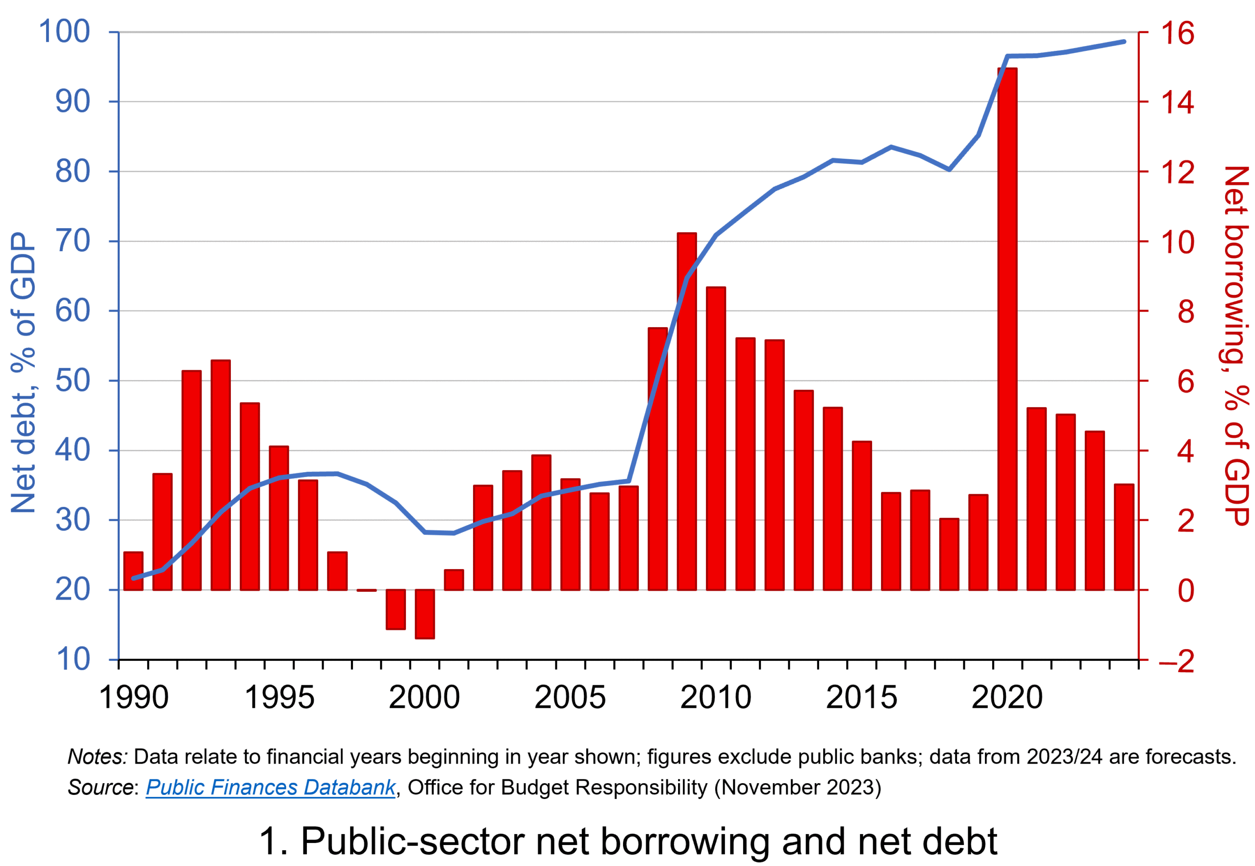Chart 1 shows the path of UK public-sector net debt and net borrowing, as percentages of GDP, since 1990. Debt is a stock concept and is the result of accumulated flows of past borrowing. Net debt is simply gross debt less liquid financial assets, which mainly consist of foreign exchange reserves and cash deposits. Net borrowing is the headline measure of the sector’s deficit and is based on when expenditures and receipts (largely taxation) are recorded rather than when cash is actually paid or received. (Click here for a PowerPoint of Chart 1)

Chart 1 shows the impact of the fiscal interventions associated with the global financial crisis and the COVID-19 pandemic, when net borrowing rose to 10 per cent and 15 per cent of GDP respectively. The former contributed to the debt-to-GDP ratio rising from 35.6 per cent in 2007/8 to 81.6 per cent in 2014/15, while the pandemic and subsequent cost-of-living interventions contributed to the ratio rising from 85.2 per cent in 2019/20 to around 98 per cent in 2023/24.

Sustainability of the public finances

The ratcheting up of debt levels affects debt servicing costs and hence the budgetary position of government. Yet the recent increases in interest rates also raise the costs faced by governments in financing future deficits or refinancing existing debts that are due to mature. In addition, a continuation of the low economic growth that has beset the UK economy since the global financial crisis also has implications for the burden imposed on the public sector by its debts, and hence the sustainability of the public finances. After all, low growth has implications for spending commitments, and, of course, the flow of receipts.

The analysis therefore implies that the sustainability of public-sector debt is dependent on at least three factors: existing debt levels, the implied average interest rate facing the public sector on its debts, and the rate of economic growth. These three factors turn out to underpin a well-known rule relating to the fiscal arithmetic of public-sector debt. The rule is sometimes known as the ‘r – g’ rule (i.e. the interest rate minus the growth rate).

Underpinning the fiscal arithmetic that determines the path of public-sector debt is the concept of the ‘primary balance’. This is the difference between the sector’s receipts and its expenditures less its debt interest payments. A primary surplus (a positive primary balance) means that receipts exceed expenditures less debt interest payments, whereas a primary deficit (a negative primary balance) means that receipts fall short. The fiscal arithmetic necessary to prevent the debt-to-GDP ratio rising produces the following stable debt equation or ‘r – g’ rule:

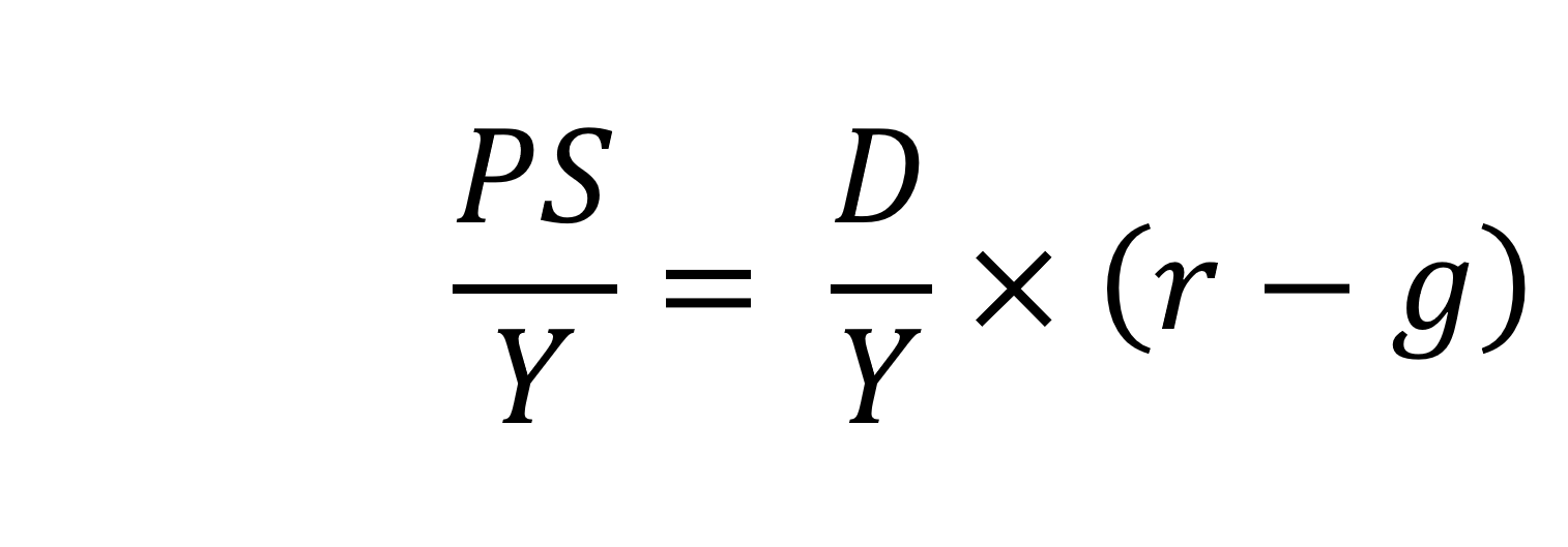
On the left-hand side of the stable debt equation is the required primary surplus (PS) to GDP (Y) ratio. Moving to the right-hand side, the first term is the existing debt-to-GDP ratio (D/Y). The second term ‘r – g’, is the differential between the average implied interest rate the government pays on its debt and the growth rate of the economy. These terms can be expressed in either nominal or real terms as this does not affect the differential.

To illustrate the rule consider a country whose existing debt-to-GDP ratio is 1 (i.e. 100 per cent) and the ‘r – g’ differential is 0.02 (2 percentage points). In this scenario they would need to run a primary surplus to GDP ratio of 0.02 (i.e. 2 percent of GDP).

The ‘r – g‘ differential

The ‘r – g’ differential reflects macroeconomic and financial conditions. The fiscal arithmetic shows that these are important for the dynamics of public-sector debt. The fiscal arithmetic is straightforward when r = g as any primary deficit will cause the debt-to-GDP ratio to rise, while a primary surplus will cause the ratio to fall. The larger is g relative to r the more favourable are the conditions for the path of debt. Importantly, if the differential is negative (r < g), it is possible for the public sector to run a primary deficit, up to the amount that the stable debt equation permits.

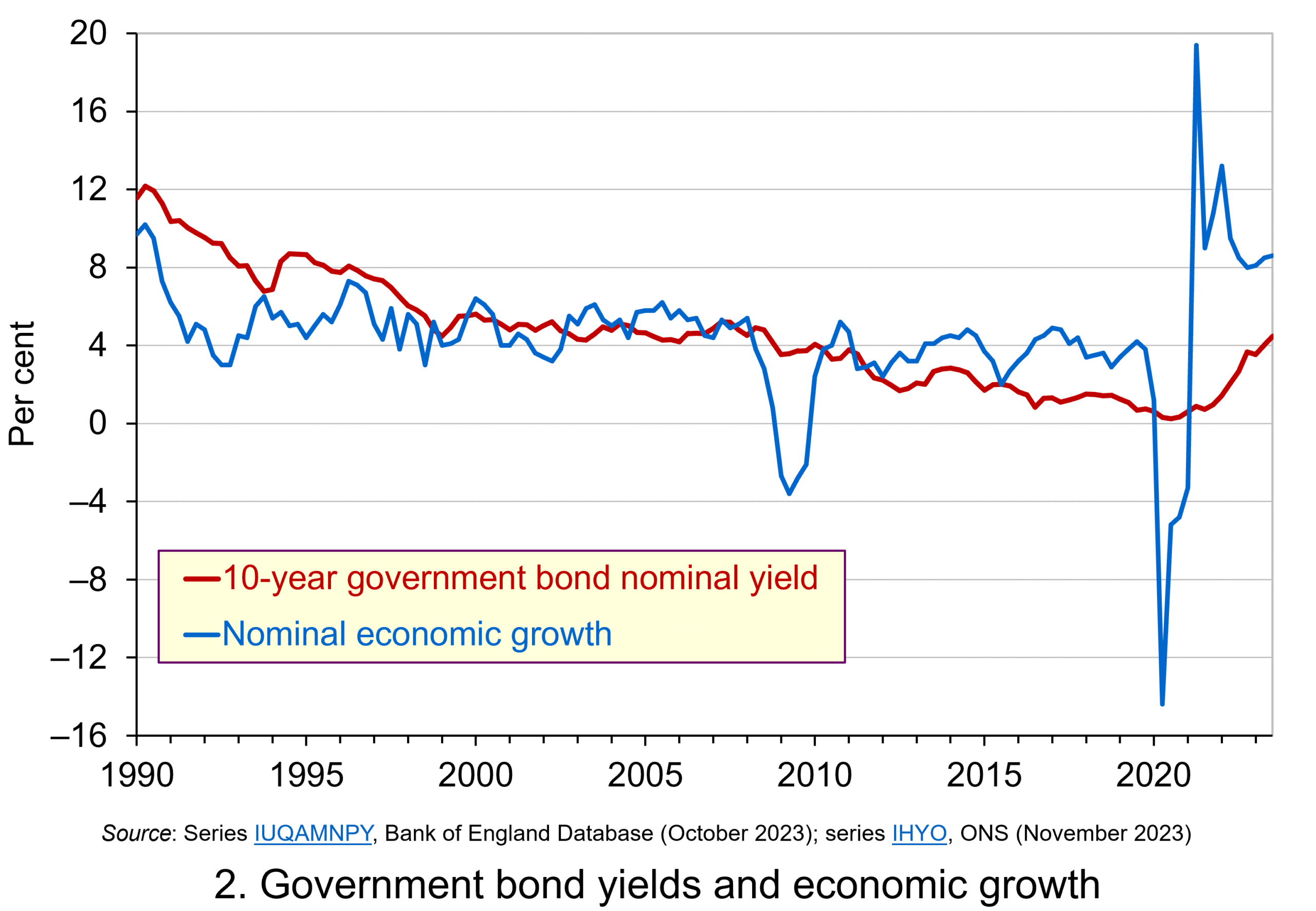Consider Charts 2 and 3 to understand how the ‘r – g’ differential has affected debt sustainability in the UK since 1990. Chart 2 plots the implied yield on 10-year government bonds, alongside the annual rate of nominal growth (click here for a PowerPoint). As John explains in his blog The bond roller coaster, the yield is calculated as the coupon rate that would have to be paid for the market price of a bond to equal its face value. Over the period, the average annual nominal growth rate was 4.5 per cent, while the implied interest rate was almost identical at 4.6 per cent. The average annual rate of CPI inflation over this period was 2.8 per cent.

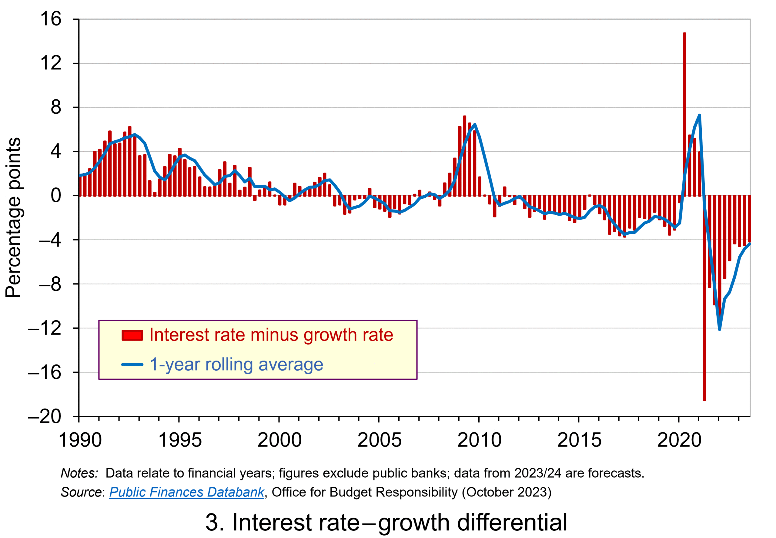Chart 3 plots the ‘r – g’ differential which is simply the difference between the two series in Chart 2, along with a 12-month rolling average of the differential to help show better the direction of the differential by smoothing out some of the short-term volatility (click here for a PowerPoint). The differential across the period is a mere 0.1 percentage points implying that macroeconomic and financial conditions have typically been neutral in supporting debt sustainability. However, this does mask some significant changes across the period.

We observe a general downward trend in the ‘r – g’ differential from 1990 up to the time of the global financial crisis. Indeed between 2003 and 2007 we observe a favourable negative differential which helps to support the sustainability of public debt and therefore the well-being of the public finances. This downward trend of the ‘r – g’ differential was interrupted by the financial crisis, driven by a significant contraction in economic activity. This led to a positive spike in the differential of over 7 percentage points.

Yet the negative differential resumed in 2010 and continued up to the pandemic. Again, this is indicative of the macroeconomic and financial environments being supportive of the public finances. It was, however, largely driven by low interest rates rather than by economic growth.

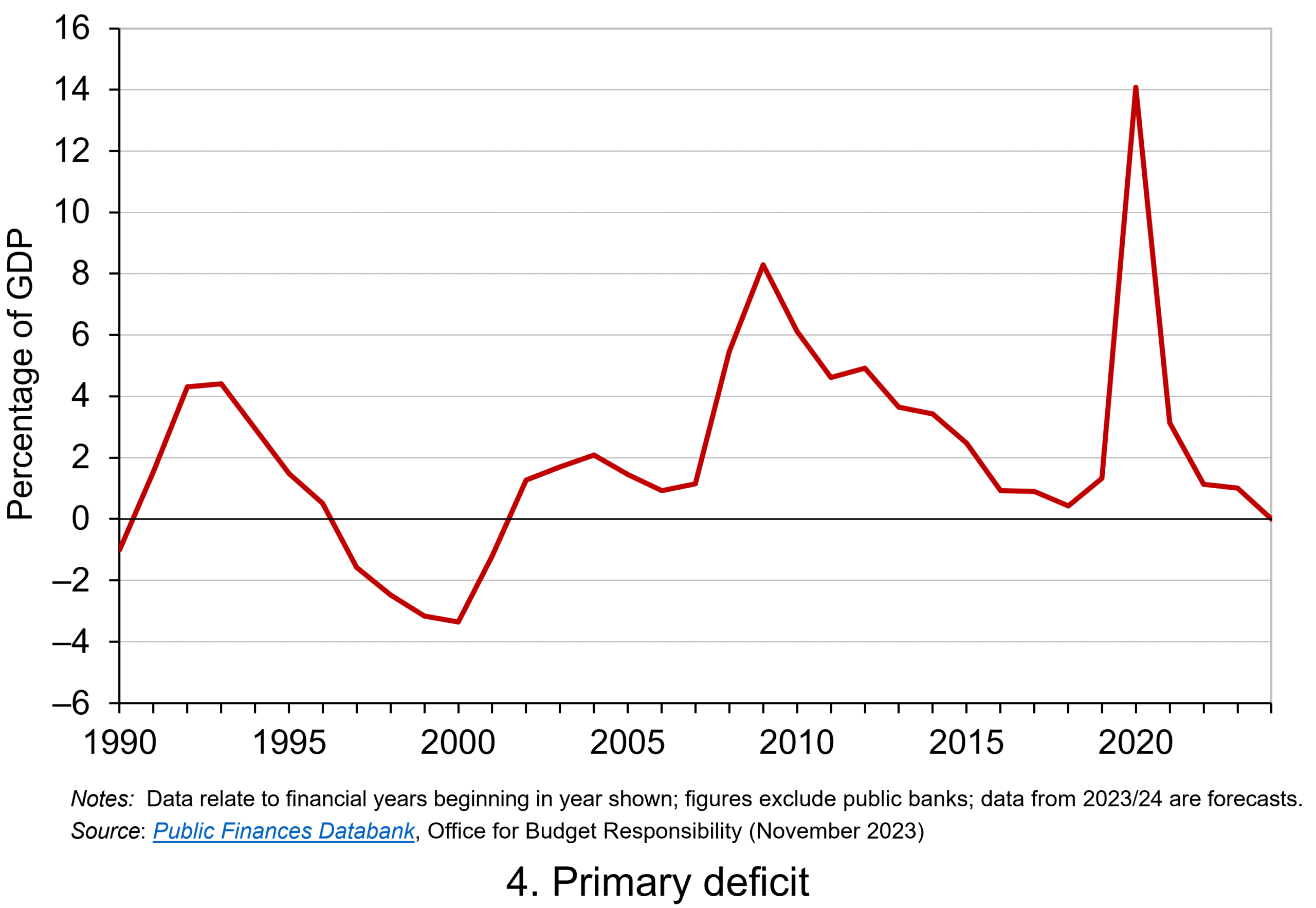
Consequently, the negative ‘r – g’ differential meant that the public sector could continue to run primary deficits during the 2010s, despite the now much higher debt-to-GDP ratio. Yet, weak growth was placing limits on this. Chart 4 indeed shows that primary deficits fell across the decade (click here for a PowerPoint).

The pandemic and beyond

The pandemic saw the ‘r – g’ differential again turn markedly positive, averaging 7 percentage points in the four quarters from Q2 of 2020. While the differential again turned negative, the debt-to-GDP ratio had also increased substantially because of large-scale fiscal interventions. This made the negative differential even more important for the sustainability of the public finances. The question is how long the negative differential can last.

Looking forward, the fiscal arithmetic is indeed uncertain and worryingly is likely to be less favourable. Interest rates have risen and, although inflationary pressures may be easing somewhat, interest rates are likely to remain much higher than during the past decade. Geopolitical tensions and global fragmentation pose future inflationary concerns and a further drag on growth.

As well as the short-term concerns over growth, there remain long-standing issues of low productivity which must be tackled if the growth of the UK economy’s potential output is to be raised. These concerns all point to the important ‘r – g’ differential become increasingly less negative, if not positive. If so the fiscal arithmetic could mean increasingly hard maths for policymakers.

Articles

• The budget deficit: a short guide

House of Commons Library (8/6/23)

• If markets are right about long real rates, public debt ratios will increase for some time. We must make sure that they do not explode.

Peterson Institute for International Economics, Olivier Blanchard (6/11/23)

• The UK government’s debt nightmare

ITV News, Robert Peston (13/7/23)

• National debt could hit 300% of GDP by 2070s, independent watchdog the OBR warns

Sky News, James Sillars (13/7/23)

• How much money is the UK government borrowing, and does it matter?

BBC News (20/10/23)

• Cost of national debt hits 20-year high

BBC News, Vishala Sri-Pathma & Faisal Islam (4/10/23)

• Bond markets could see ‘mini boom-bust cycles’ as global government debt to soar by $5 trillion a yea

Markets Insider, Filip De Mott (16/11/23)

• The counterintuitive truth about deficits for bond investors

Financial Times, Matt King (17/11/23)

• UK government borrowing almost £20bn lower than expected

The Guardian, Richard Partington (20/10/23)

• Controlling debt is just a means — it is not a government’s end

Financial Times, Martin Wolf (13/11/23)

Data

• Public finances databank

Office for Budget Responsibility

• Bonds

Financial Times

• Gilt market data

UK Debt Management Office

• Yields on British Government Stock

Bank of England

Questions