 According to the IMF, Chinese GDP grew by 5.2% in 2023 and is predicted to grow by 4.6% this year. Such growth rates would be extremely welcome to most developed countries. UK growth in 2023 was a mere 0.5% and is forecast to be only 0.6% in 2024. Advanced economies as a whole only grew by 1.6% in 2023 and are forecast to grow by only 1.5% this year. Also, with the exception of India, the Philippines and Indonesia, which grew by 6.7%, 5.3% and 5.0% respectively in 2023 and are forecast to grow by 6.5%, 6.0% and 5.0% this year, Chinese growth also compares very favourably with other developing countries, which as a weighted average grew by 4.1% last year and are forecast to grow at the same rate this year.
 But in the past, Chinese growth was much higher and was a major driver of global growth. Over the period 1980 to 2018, Chinese economic growth averaged 9.5% – more than twice the average rate of developing countries (4.5%) and nearly four times the average rate of advanced countries (2.4%) (see chart – click here for a PowerPoint of the chart).
Not only is Chinese growth now much lower, but it is set to decline further. The IMF forecasts that in 2025, Chinese growth will have fallen to 4.1% – below the forecast developing-country average of 4.2% and well below that of India (6.5%).
Causes of slowing Chinese growth
There are a number of factors that have come together to contribute to falling economic growth rates – growth rates that otherwise would have been expected to be considerably higher as the Chinese economy reopened after severe Covid lockdowns.
 Property market
China has experienced a property boom over the past 20 years years as the government has encouraged construction in residential blocks and in factories and offices. The sector has accounted for some 20% of economic activity. But for many years, demand outstripped supply as consumers chose to invest in property, partly because of a lack of attractive alternatives for their considerable savings and partly because property prices were expected to go on rising. This lead to speculation on the part of both buyers and property developers. Consumers rushed to buy property before prices rose further and property developers borrowed considerably to buy land, which local authorities encouraged, as it provided a valuable source of revenue.
But now there is considerable overcapacity in the sector and new building has declined over the past three years. According to the IMF:
Housing starts have fallen by more than 60 per cent relative to pre-pandemic levels, a historically rapid pace only seen in the largest housing busts in cross-country experience in the last three decades. Sales have fallen amid homebuyer concerns that developers lack sufficient financing to complete projects and that prices will decline in the future.
As a result, many property developers have become unviable. At the end of January, the Chinese property giant, Evergrande, was ordered to liquidate by a Hong Kong court, after the judge ruled that the company did not have a workable plan to restructure around $300bn of debt. Over 50 Chinese property developers have defaulted or missed payments since 2020. The liquidation of Evergrande and worries about the viability of other Chinese property developers is likely to send shockwaves around the Chinese property market and more widely around Chinese investment markets.
Overcapacity
Rapid investment over many years has led to a large rise in industrial capacity. This has outstripped demand. The problem could get worse as investment, including state investment, is diverted from the property sector to manufacturing, especially electric vehicles. But with domestic demand dampened, this could lead to increased dumping on international markets – something that could spark trade wars with the USA and other trading partners (see below). Worries about this in China are increasing as the possibility of a second Trump presidency looks more possible. The Chinese authorities are keen to expand aggregate demand to tackle this overcapacity.
Uncertainty
Consumer and investor confidence are low. This is leading to severe deflationary pressures. If consumers face a decline in the value of their property, this wealth effect could further constrain their spending. This will, in turn, dampen industrial investment.
Uncertainty is beginning to affect foreign companies based in China. Many foreign companies are now making a loss in China or are at best breaking even. This could lead to disinvestment and add to deflationary pressures.
The Chinese stock market and policy responses
 Lack of confidence in the Chinese economy is reflected in falling share prices. The Shanghai SSE Composite Index (an index of all stocks traded on the Shanghai Stock Exchange) has fallen dramatically in recent months. From a high of 3703 in September 2021, it had fallen to 2702 on 5 Feb 2024 – a fall of 27%. It is now below the level at the beginning of 2010 (see chart: click here for a PowerPoint). On 5 February alone, some 1800 stocks fell by over 10% in Shanghai and Shenzhen. People were sensing a rout and investors expressed their frustration and anger on social media, including the social media account of the US Embassy. The next day, the authorities intervened and bought large quantities of key stocks. China’s sovereign wealth fund announced that it would increase its purchase of shares to support the country’s stock markets. The SSE Composite rose 4.1% on 6 February and the Shenzhen Component Index rose 6.2%.
However, the rally eased as investors waited to see what more fundamental measures the authorities would take to support the stock markets and the economy more generally. Policies are needed to boost the wider economy and encourage a growth in consumer and business confidence.
Interest rates have been cut four times since the beginning of 2022, when the prime loan rate was cut from 3.85% to 3.7%. The last cut was from 3.55% to 3.45% in August 2023. But this has been insufficient to provide the necessary boost to aggregate demand. Further cuts in interest rates are possible and the government has said that it will use proactive fiscal and effective monetary policy in response to the languishing economy. However, government debt is already high, which limits the room for expansionary fiscal policy, and consumers are highly risk averse and have a high propensity to save.
Graduate unemployment
 China has seen investment in education as an important means of increasing human capital and growth. But with a slowing economy, there are are more young people graduating each year than there are graduate jobs available. Official data show that for the group aged 16–24, the unemployment rate was 14.9% in December. This compares with an overall urban unemployment rate of 5.1%. Many graduates are forced to take non-graduate jobs and graduate jobs are being offered at reduced salaries. This will have a further dampening effect on aggregate demand.
Demographics
China’s one-child policy, which it pursued from 1980 to 2016, plus improved health and social care leading to greater longevity, has led to an ageing population and a shrinking workforce. This is despite recent increases in unemployment in the 16–24 age group. The greater the ratio of dependants to workers, the greater the brake on growth as taxes and savings are increasingly used to provide various forms of support.
Effects on the rest of the world
China has been a major driver of world economic growth. With a slowing Chinese economy, this will provide less stimulus to growth in other countries. Many multinational companies, including chip makers, cosmetics companies and chemical companies, earn considerable revenue from China. For example, the USA exports over $190 billion of goods and services to China and these support over 1 million jobs in the USA. A slowdown in China will have repercussions for many companies around the world.
There is also the concern that Chinese manufacturers may dump products on world markets at less than average (total) cost to shift stock and keep production up. This could undermine industry in many countries and could initiate a protectionist response. Already Donald Trump is talking about imposing a 10% tariff on most imported goods if he is elected again in November. Such tariffs could be considerably higher on imports from China. If Joe Biden is re-elected, he too may impose tariffs on Chinese goods if they are thought to be unfairly subsidised. US (and possibly EU) tariffs on Chinese goods could lead to a similar response from China, resulting in a trade war – a negative sum game.
Videos
Articles
- IMF Predicts China Economy Slowing Over Next Four Years
Voice of America, Evie Steele (2/2/24)
- China’s Real Estate Sector: Managing the Medium-Term Slowdown
IMF News, Henry Hoyle and Sonali Jain-Chandra (2/2/24)
- China braced for largest human migration on earth amid bleak economic backdrop
ITV News, Debi Edward (4/2/24)
- China’s property giant Evergrande ordered to liquidate as debt talks fail
Aljazeera (29/1/24)
- China’s overcapacity a challenge that is ‘here to stay’, says US chamber
Financial Times, Joe Leahy (1/2/24)
- China needs to learn lessons from 1990s Japan
Financial Times, Gillian Tett (1/2/24)
- The Trump factor is looming over China’s markets
Financial Times, Katie Martin (2/2/24)
- China’s many systemic problems dominate its outlook for 2024
The Guardian, George Magnus (1/1/24)
- China youth unemployment will stay elevated in 2024, but EIU warns economic impact will linger
CNBC, Clement Tan (25/1/24)
- Don’t count on a soft landing for the world economy – turbulence is ahead
The Guardian, Kenneth Rogoff (2/2/24)
- As falling stocks draw criticism in China, censors struggle to keep up
Washington Post, Lily Kuo (6/2/24)
- China’s doom loop: a dramatically smaller (and older) population could create a devastating global slowdown
The Conversation, Jose Caballero (12/2/24)
- China: why the country’s economy has hit a wall – and what it plans to do about it
The Conversation, Hong Bo (19/3/24)
- Confronting inflation and low growth
OECD Economic Outlook Interim Report (September 2023) (see especially Box 1)
Questions
- Why is China experiencing slowing growth and is growth likely to pick up over the next five years?
- How does the situation in China today compare with that in Japan 30 years ago?
- What policies could the Chinese government pursue to stimulate economic growth?
- What policies were enacted towards China during the Trump presidency from 2017 to 2020?
- Would you advise the Chinese central bank to cut interest rates further? Explain.
- Should China introduce generous child support for families, no matter the number of children?
 The past decade or so has seen large-scale economic turbulence. As we saw in the blog Fiscal impulses, governments have responded with large fiscal interventions. The COVID-19 pandemic, for example, led to a positive fiscal impulse in the UK in 2020, as measured by the change in the structural primary balance, of over 12 per cent of national income.
The scale of these interventions has led to a significant increase in the public-sector debt-to-GDP ratio in many countries. The recent interest rates hikes arising from central banks responding to inflationary pressures have put additional pressure on the financial well-being of governments, not least on the financing of their debt. Here we discuss these pressures in the context of the ‘r – g’ rule of sustainable public debt.
Public-sector debt and borrowing
 Chart 1 shows the path of UK public-sector net debt and net borrowing, as percentages of GDP, since 1990. Debt is a stock concept and is the result of accumulated flows of past borrowing. Net debt is simply gross debt less liquid financial assets, which mainly consist of foreign exchange reserves and cash deposits. Net borrowing is the headline measure of the sector’s deficit and is based on when expenditures and receipts (largely taxation) are recorded rather than when cash is actually paid or received. (Click here for a PowerPoint of Chart 1)
Chart 1 shows the impact of the fiscal interventions associated with the global financial crisis and the COVID-19 pandemic, when net borrowing rose to 10 per cent and 15 per cent of GDP respectively. The former contributed to the debt-to-GDP ratio rising from 35.6 per cent in 2007/8 to 81.6 per cent in 2014/15, while the pandemic and subsequent cost-of-living interventions contributed to the ratio rising from 85.2 per cent in 2019/20 to around 98 per cent in 2023/24.
Sustainability of the public finances
") The ratcheting up of debt levels affects debt servicing costs and hence the budgetary position of government. Yet the recent increases in interest rates also raise the costs faced by governments in financing future deficits or refinancing existing debts that are due to mature. In addition, a continuation of the low economic growth that has beset the UK economy since the global financial crisis also has implications for the burden imposed on the public sector by its debts, and hence the sustainability of the public finances. After all, low growth has implications for spending commitments, and, of course, the flow of receipts.
The ratcheting up of debt levels affects debt servicing costs and hence the budgetary position of government. Yet the recent increases in interest rates also raise the costs faced by governments in financing future deficits or refinancing existing debts that are due to mature. In addition, a continuation of the low economic growth that has beset the UK economy since the global financial crisis also has implications for the burden imposed on the public sector by its debts, and hence the sustainability of the public finances. After all, low growth has implications for spending commitments, and, of course, the flow of receipts.
The analysis therefore implies that the sustainability of public-sector debt is dependent on at least three factors: existing debt levels, the implied average interest rate facing the public sector on its debts, and the rate of economic growth. These three factors turn out to underpin a well-known rule relating to the fiscal arithmetic of public-sector debt. The rule is sometimes known as the ‘r – g’ rule (i.e. the interest rate minus the growth rate).
Underpinning the fiscal arithmetic that determines the path of public-sector debt is the concept of the ‘primary balance’. This is the difference between the sector’s receipts and its expenditures less its debt interest payments. A primary surplus (a positive primary balance) means that receipts exceed expenditures less debt interest payments, whereas a primary deficit (a negative primary balance) means that receipts fall short. The fiscal arithmetic necessary to prevent the debt-to-GDP ratio rising produces the following stable debt equation or ‘r – g’ rule:
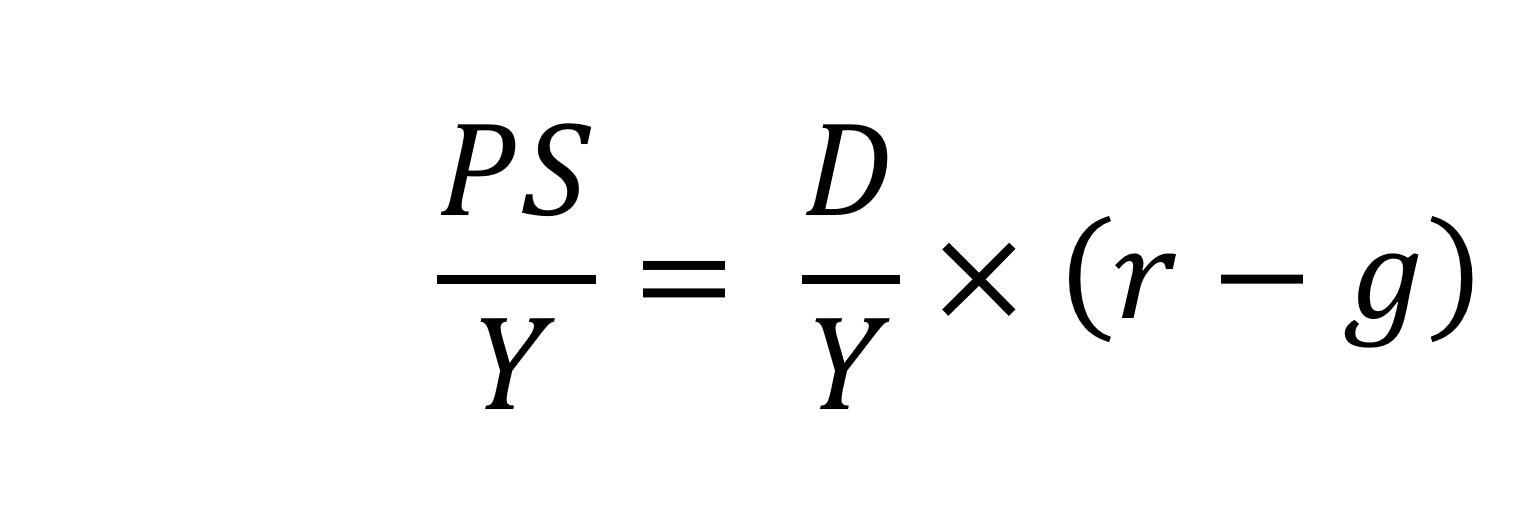
On the left-hand side of the stable debt equation is the required primary surplus (PS) to GDP (Y) ratio. Moving to the right-hand side, the first term is the existing debt-to-GDP ratio (D/Y). The second term ‘r – g’, is the differential between the average implied interest rate the government pays on its debt and the growth rate of the economy. These terms can be expressed in either nominal or real terms as this does not affect the differential.
To illustrate the rule consider a country whose existing debt-to-GDP ratio is 1 (i.e. 100 per cent) and the ‘r – g’ differential is 0.02 (2 percentage points). In this scenario they would need to run a primary surplus to GDP ratio of 0.02 (i.e. 2 percent of GDP).
The ‘r – g‘ differential
The ‘r – g’ differential reflects macroeconomic and financial conditions. The fiscal arithmetic shows that these are important for the dynamics of public-sector debt. The fiscal arithmetic is straightforward when r = g as any primary deficit will cause the debt-to-GDP ratio to rise, while a primary surplus will cause the ratio to fall. The larger is g relative to r the more favourable are the conditions for the path of debt. Importantly, if the differential is negative (r < g), it is possible for the public sector to run a primary deficit, up to the amount that the stable debt equation permits.
 Consider Charts 2 and 3 to understand how the ‘r – g’ differential has affected debt sustainability in the UK since 1990. Chart 2 plots the implied yield on 10-year government bonds, alongside the annual rate of nominal growth (click here for a PowerPoint). As John explains in his blog The bond roller coaster, the yield is calculated as the coupon rate that would have to be paid for the market price of a bond to equal its face value. Over the period, the average annual nominal growth rate was 4.5 per cent, while the implied interest rate was almost identical at 4.6 per cent. The average annual rate of CPI inflation over this period was 2.8 per cent.
 Chart 3 plots the ‘r – g’ differential which is simply the difference between the two series in Chart 2, along with a 12-month rolling average of the differential to help show better the direction of the differential by smoothing out some of the short-term volatility (click here for a PowerPoint). The differential across the period is a mere 0.1 percentage points implying that macroeconomic and financial conditions have typically been neutral in supporting debt sustainability. However, this does mask some significant changes across the period.
We observe a general downward trend in the ‘r – g’ differential from 1990 up to the time of the global financial crisis. Indeed between 2003 and 2007 we observe a favourable negative differential which helps to support the sustainability of public debt and therefore the well-being of the public finances. This downward trend of the ‘r – g’ differential was interrupted by the financial crisis, driven by a significant contraction in economic activity. This led to a positive spike in the differential of over 7 percentage points.
 Yet the negative differential resumed in 2010 and continued up to the pandemic. Again, this is indicative of the macroeconomic and financial environments being supportive of the public finances. It was, however, largely driven by low interest rates rather than by economic growth.
Consequently, the negative ‘r – g’ differential meant that the public sector could continue to run primary deficits during the 2010s, despite the now much higher debt-to-GDP ratio. Yet, weak growth was placing limits on this. Chart 4 indeed shows that primary deficits fell across the decade (click here for a PowerPoint).
The pandemic and beyond
 The pandemic saw the ‘r – g’ differential again turn markedly positive, averaging 7 percentage points in the four quarters from Q2 of 2020. While the differential again turned negative, the debt-to-GDP ratio had also increased substantially because of large-scale fiscal interventions. This made the negative differential even more important for the sustainability of the public finances. The question is how long the negative differential can last.
Looking forward, the fiscal arithmetic is indeed uncertain and worryingly is likely to be less favourable. Interest rates have risen and, although inflationary pressures may be easing somewhat, interest rates are likely to remain much higher than during the past decade. Geopolitical tensions and global fragmentation pose future inflationary concerns and a further drag on growth.
As well as the short-term concerns over growth, there remain long-standing issues of low productivity which must be tackled if the growth of the UK economy’s potential output is to be raised. These concerns all point to the important ‘r – g’ differential become increasingly less negative, if not positive. If so the fiscal arithmetic could mean increasingly hard maths for policymakers.
Articles
- The budget deficit: a short guide
House of Commons Library (8/6/23)
- If markets are right about long real rates, public debt ratios will increase for some time. We must make sure that they do not explode.
Peterson Institute for International Economics, Olivier Blanchard (6/11/23)
- The UK government’s debt nightmare
ITV News, Robert Peston (13/7/23)
- National debt could hit 300% of GDP by 2070s, independent watchdog the OBR warns
Sky News, James Sillars (13/7/23)
- How much money is the UK government borrowing, and does it matter?
BBC News (20/10/23)
- Cost of national debt hits 20-year high
BBC News, Vishala Sri-Pathma & Faisal Islam (4/10/23)
- Bond markets could see ‘mini boom-bust cycles’ as global government debt to soar by $5 trillion a yea
Markets Insider, Filip De Mott (16/11/23)
- The counterintuitive truth about deficits for bond investors
Financial Times, Matt King (17/11/23)
- UK government borrowing almost £20bn lower than expected
The Guardian, Richard Partington (20/10/23)
- Controlling debt is just a means — it is not a government’s end
Financial Times, Martin Wolf (13/11/23)
Data
Questions
- What is meant by each of the following terms: (a) net borrowing; (b) primary deficit; (c) net debt?
- Explain how the following affect the path of the public-sector debt-to-GDP ratio: (a) interest rates; (b) economic growth; (c) the existing debt-to-GDP ratio.
- Which factors during the 2010s were affecting the fiscal arithmetic of public debt positively, and which negatively?
- Discuss the prospects for the fiscal arithmetic of public debt in the coming years.
- Assume that a country has an existing public-sector debt-to-GDP ratio of 60 percent.
(a) Using the ‘rule of thumb’ for public debt dynamics, calculate the approximate primary balance it would need to run in the coming year if the expected average real interest rate on the debt were 3 per cent and real economic growth were 2 per cent?
(b) Repeat (a) but now assume that real economic growth is expected to be 4 per cent.
(c) Repeat (a) but now assume that the existing public-sector debt-to-GDP ratio is 120 per cent.
(d) Using your results from (a) to (c) discuss the factors that affect the fiscal arithmetic of the growth of public-sector debt.
 In his blog, The bond roller coaster, John looks at the pricing of government bonds and details how, in recent times, governments wishing to borrow by issuing new bonds are having to offer higher coupon rates to attract investors. The interest rate hikes by central banks in response to global-wide inflationary pressures have therefore spilt over into bond markets. Though this evidences the ‘pass through’ of central bank interest rate increases to the general structure of interest rates, it does, however, pose significant costs for governments as they seek to finance future budgetary deficits or refinance existing debts coming up to maturity.
The Autumn Statement in the UK is scheduled to be made on 22 November. This, as well as providing an update on the economy and the public finances, is likely to include a number of fiscal proposals. It is thus timely to remind ourselves of the size of recent discretionary fiscal measures and their potential impact on the sustainability of the public finances. In this first of two blogs, we consider the former: the magnitude of recent discretionary fiscal policy changes.
First, it is important to define what we mean by discretionary fiscal policy. It refers to deliberate changes in government spending or taxation. This needs to be distinguished from the concept of automatic stabilisers, which relate to those parts of government budgets that automatically result in an increase (decrease) of spending or a decrease (increase) in tax payments when the economy slows (quickens).
The suitability of discretionary fiscal policy measures depends on the objectives they trying to fulfil. Discretionary measures can be implemented, for example, to affect levels of public-service provision, the distribution of income, levels of aggregate demand or to affect longer-term growth of aggregate supply. As we shall see in this blog, some of the large recent interventions have been conducted primarily to support and stabilise economic activity in the face of heightened economic volatility.
 Discretionary fiscal measures in the UK are usually announced in annual Budget statements in the House of Commons. These are normally in March, but discretionary fiscal changes can be made in the Autumn Statement too. The Autumn Statement of October 2022, for example, took on significant importance as the new Chancellor of the Exchequer, Jeremy Hunt, tried to present a ‘safe pair hands’ following the fallout and market turbulence in response to the fiscal statement by the former Chancellor, Kwasi Kwarteng, on 23 September that year.
The fiscal impulse
The large-scale economic turbulence of recent years associated first with the global financial crisis of 2007–9 and then with the COVID-19 pandemic and the cost-of-living crisis, has seen governments respond with significant discretionary fiscal measures. During the COVID-19 pandemic, examples of fiscal interventions in the UK included the COVID-19 Business Interruption Loan Scheme (CBILS), grants for retail, hospitality and leisure businesses, the COVID-19 Job Retention Scheme (better known as the furlough scheme) and the Self-Employed Income Support Scheme.
 The size of discretionary fiscal interventions can be measured by the fiscal impulse. This captures the magnitude of change in discretionary fiscal policy and thus the size of the stimulus. The concept is not to be confused with fiscal multipliers, which measure the impact of fiscal changes on economic outcomes, such as real national income and employment.
By measuring fiscal impulses, we can analyse the extent to which a country’s fiscal stance has tightened, loosened, or remained unchanged. In other words, we are attempting to capture discretionary fiscal policy changes that result in structural changes in the government budget and, therefore, in structural changes in spending and/or taxation.
To measure structural changes in the public-sector’s budgetary position, we calculate changes in structural budget balances.
A budget balance is simply the difference between receipts (largely taxation) and spending. A budget surplus occurs when receipts are greater than spending, while a deficit (sometimes referred to as net borrowing) occurs if spending is greater than receipts.
A structural budget balance cyclically-adjusts receipts and spending and hence adjusts for the position of the economy in the business cycle. In doing so, it has the effect of adjusting both receipts and spending for the effect of automatic stabilisers. Another way of thinking about this is to ask what the balance between receipts and spending would be if the economy were operating at its potential output. A deterioration in a structural budget balance infers a rise in the structural deficit or fall in the structural surplus. This indicates a loosening of the fiscal stance. An improvement in the structural budget balance, by contrast, indicates a tightening.
The size of UK fiscal impulses
A frequently-used measure of the fiscal impulse involves the change in the cyclically-adjusted public-sector primary deficit.
 A primary deficit captures the extent to which the receipts of the public sector fall short of its spending, excluding its spending on debt interest payments. It essentially captures whether the public sector is able to afford its ‘new’ fiscal choices from its receipts; it excludes debt-servicing costs, which can be thought of as reflecting fiscal choices of the past. By using a cyclically-adjusted primary deficit we are able to isolate more accurately the size of discretionary policy changes. Chart 1 shows the UK’s actual and cyclically-adjusted primary deficit as a share of GDP since 1975, which have averaged 1.3 and 1.1 per cent of GDP respectively. (Click here for a PowerPoint of the chart.)
The size of the fiscal impulse is measured by the year-on-year percentage point change in the cyclically-adjusted public-sector primary deficit as a percentage of GDP. A larger deficit or a smaller surplus indicates a fiscal loosening (a positive fiscal impulse), while a smaller deficit or a larger surplus indicates a fiscal tightening (a negative fiscal impulse).
 Chart 2 shows the magnitude of UK fiscal impulses since 1980. It captures very starkly the extent of the loosening of the fiscal stance in 2020 in response to the COVID-19 pandemic. (Click here for a PowerPoint of the chart.) In 2020 the cyclically-adjusted primary deficit to GDP ratio rose from 1.67 to 14.04 per cent. This represents a positive fiscal impulse of 12.4 per cent of GDP.
A tightening of fiscal policy followed the waning of the pandemic. 2021 saw a negative fiscal impulse of 10.1 per cent of GDP. Subsequent tightening was tempered by policy measures to limit the impact on the private sector of the cost-of-living crisis, including the Energy Price Guarantee and Energy Bills Support Scheme.
In comparison, the fiscal response to the global financial crisis led to a cumulative increase in the cyclically-adjusted primary deficit to GDP ratio from 2007 to 2009 of 5.0 percentage points. Hence, the financial crisis saw a positive fiscal impulse of 5 per cent of GDP. While smaller in comparison to the discretionary fiscal responses to the COVID-19 pandemic, it was, nonetheless, a sizeable loosening of the fiscal stance.
Sustainability and well-being of the public finances
The recent fiscal interventions have implications for the financial well-being of the public-sector. Not least, the financing of the positive fiscal impulses has led to a substantial growth in the accumulated size of the public-sector debt stock. At the end of 2006/7 the public-sector net debt stock was 35 per cent of GDP; at the end of the current financial year, 2023/24, it is expected to be 103 per cent.
As we saw at the outset, in an environment of rising interest rates, the increase in the public-sector debt to GDP ratio creates significant additional costs for government, a situation that is made more difficult for government not only by the current flatlining of economic activity, but by the low underlying rate of economic growth seen since the financial crisis. The combination of higher interest rates and lower economic growth has adverse implications for the sustainability of the public finances and the ability of the public sector to absorb the effects of future economic crises.
Articles
- Autumn Statement 2023: When is it and how will it affect me?
BBC News (16/11/23)
- What is the Autumn Statement?
House of Commons Library (13/11/23)
- Putting the fiscal toothpaste back into the tube: It’s time to normalise the euro area fiscal stance in 2024
VoxEU, Niels Thygesen, Roel Beetsma, Massimo Bordignon, Xavier Debrun, Mateusz Szczurek, Martin Larch, Matthias Busse, Mateja Gabrijelcic, Laszlo Jankovics and Janis Malzubris (30/6/23)
- Euro zone should tighten fiscal policy in 2024 to curb inflation, European Fiscal Board says
Reuters, Jan Strupczewski (28/6/23)
- Hutchins Center Fiscal Impact Measure: Federal, State and Local Fiscal Policy and the Economy
Brookings, Eli Asdourian, Louise Sheiner, and Lorae Stojanovic (27/10/23)
Report
- IFS Green Budget
Institute for Fiscal Studies, Carl Emmerson, Paul Johnson and Ben Zaranko (eds) (October 2023)
Data
Questions
- Explain what is meant by the following fiscal terms: (a) structural deficit; (b) automatic stabilisers; (c) discretionary fiscal policy; (d) primary deficit.
- What is the difference between current and capital public expenditures? Give some examples of each.
- Consider the following two examples of public expenditure: grants from government paid to the private sector for the installation of energy-efficient boilers, and welfare payments to unemployed people. How are these expenditures classified in the public finances and what fiscal objectives do you think they meet?
- Which of the following statements about the primary balance is FALSE?
(a) In the presence of debt interest payments a primary deficit will be smaller than a budget deficit.
(b) In the presence of debt interest payments a primary surplus will be smaller than a budget surplus.
(c) The primary balance differs from the budget balance by the size of debt interest payments.
(d) None of the above.
- Explain the difference between a fiscal impulse and a fiscal multiplier.
- Why is low economic growth likely to affect the sustainability of the public finances? What other factors could also matter?
To finance budget deficits, governments have to borrow. They can borrow short-term by issuing Treasury bills, typically for 1, 3 or 6 months. These do not earn interest and hence are sold at a discount below the face value. The rate of discount depends on supply and demand and will reflect short-term market rates of interest. Alternatively, governments can borrow long-term by issuing bonds. In the UK, these government securities are known as ‘gilts’ or ‘gilt-edged securities’. In the USA they are known as ‘treasury bonds’, ‘T-bonds’ or simply ‘treasuries’. In the EU, countries separately issue bonds but the European Commission also issues bonds.
In the UK, gilts are issued by the Debt Management Office on behalf of the Treasury. Although there are index-linked gilts, the largest proportion of gilts are conventional gilts. These pay a fixed sum of money per annum per £100 of face value. This is known as the ‘coupon payment’ and the rate is set at the time of issue. The ‘coupon rate’ is the payment per annum as a percentage of the bond’s face value:

Payments are made six-monthly. Each issue also has a maturity date, at which point the bonds will be redeemed at face value. For example, a 4½% Treasury Gilt 2028 bond has a coupon rate of 4½% and thus pays £4.50 per annum (£2.25 every six months) for each £100 of face value. The issue will be redeemed in June 2028 at face value. The issue was made in June 2023 and thus represented a 5-year bond. Gilts are issued for varying lengths of time from 2 to 55 years. At present, there are 61 different conventional issues of bonds, with maturity dates varying from January 2024 to October 2073.
Bond prices
 Bonds can be sold on the secondary market (i.e. the stock market) before maturity. The market price, however, is unlikely to be the coupon price (i.e. the face value). The lower the coupon rate relative to current interest rates, the less valuable the bond will be. For example, if interest rates rise, and hence new bonds pay a higher coupon rate, the market price of existing bonds paying a lower coupon rate must fall. Thus bond prices vary inversely with interest rates.
The market price also depends on how close the bonds are to maturity. The closer the maturity date, the closer the market price of the bond will be to the face value.
Bond yields: current yield
A bond’s yield is the percentage return that a person buying the bond receives. If a newly issued bond is bought at the coupon price, its yield is the coupon rate.
However, if an existing bond is bought on the secondary market (the stock market), the yield must reflect the coupon payments relative to the purchase price, not the coupon price. We can distinguish between the ‘current yield’ and the ‘yield to maturity’.
The current yield is the coupon payment as a percentage of the current market price of the bond:

Assume a bond were originally issued at 2% (its coupon rate) and thus pays £2 per annum. In the meantime, however, assume that interest rates have risen and new bonds now have a coupon rate of 4%, paying £4 per annum for each £100 invested. To persuade people to buy old bonds with a coupon rate of 2%, their market prices must fall below their face value (their coupon price). If their price halved, then they would pay £2 for every £50 of their market price and hence their current yield would be 4% (£2/£50 × 100).
Bond yields: yield to maturity (YTM)
But the current yield does not give the true yield – it is only an approximation. The true yield must take into account not just the market price but also the maturity value and the length of time to maturity (and the frequency of payments too, which we will ignore here). The closer a bond is to its maturity date, the higher/lower will be the true yield if the price is below/above the coupon price: in other words, the closer will the market price be to the coupon price for any given market rate of interest.
A more accurate measure of a bond’s yield is thus the ‘yield to maturity’ (YTM). This is the interest rate which makes the present value of all a bond’s future cash flows equal to its current price. These cash flows include all coupon payments and the payment of the face value on maturity. But future cash flows must be discounted to take into account the fact that money received in the future is worth less than money received now, since money received now could then earn interest.
The yield to maturity is the internal rate of return (IRR) of the bond. This is the discount rate which makes the present value (PV) of all the bond’s future cash flows (including the maturity payment of the coupon price) equal to its current market price. For simplicity, we assume that coupon payments are made annually. The formula is the one where the bond’s current market price is given by:

Where: t is the year; n is the number of years to maturity; YTM is the yield to maturity.
Thus if a bond paid £5 each year and had a maturity value of £100 and if current interest rates were higher than 5%, giving a yield to maturity of 8%, then the bond price would be:

In other words, with a coupon rate of 5% and a higher YTM of 8%, the bond with a face value of £100 and five years to maturity would be worth only £88.02 today.
If you know the market price of a given bond, you can work out its YTM by substituting in the above formula. The following table gives examples.

The higher the YTM, the lower the market price of a bond. Since the YTM reflects in part current rates of interest, so the higher the rate of interest, the lower the market price of any given bond. Thus bond yields vary directly with interest rates and bond prices vary inversely. You can see this clearly from the table. You can also see that market bond prices converge on the face value as the maturity date approaches.
Recent activity in bond markets
Investing in government bonds is regarded as very safe. Coupon payments are guaranteed, as is repayment of the face value on the maturity date. For this reason, many pension funds hold a lot of government bonds issued by financially trustworthy governments. But in recent months, bond prices in the secondary market have fallen substantially as interest rates have risen. For those holding existing bonds, this means that their value has fallen. For governments wishing to borrow by issuing new bonds, the cost has risen as they have to offer a higher coupon rate to attract buyers. This make it more expensive to finance government debt.
 The chart shows the yield on 10-year government bonds. It is calculated using the ‘par value’ approach. This gives the coupon rate that would have to be paid for the market price of a bond to equal its face value. Clearly, as interest rates rise, a bond would have to pay a higher coupon rate for this to happen. (This, of course, is only hypothetical to give an estimate of market rates, as coupon rates are fixed at the time of a bond’s issue.)
Par values reflect both yield to maturity and also expectations of future interest rates. The higher people expect future interest rates to be, the higher must par values be to reflect this.
 In the years following the financial crisis of 2007–8 and the subsequent recession, and again during the COVID pandemic, central banks cut interest rates and supported this by quantitative easing. This involved central banks buying existing bonds on the secondary market and paying for them with newly created (electronic) money. This drove up bond prices and drove down yields (as the chart shows). This helped support the policy of low interest rates. This was a boon to governments, which were able to borrow cheaply.
This has all changed. With quantitative tightening replacing quantitative easing, central banks have been engaging in asset sales, thereby driving down bond prices and driving up yields. Again, this can be seen in the chart. This has helped to support a policy of higher interest rates.
Problems of higher bond yields/lower bond prices
Although lower bond prices and higher yields have supported a tighter monetary policy, which has been used to fight inflation, this has created problems.
First, it has increased the cost of financing government debt. In 2007/8, UK public-sector net debt was £567bn (35.6% of GDP). The Office for Budget Responsibility forecasts that it will be £2702bn (103.1% of GDP in the current financial year – 2023/24). Not only, therefore, are coupon rates higher for new government borrowing, but the level of borrowing is now a much higher proportion of GDP. In 2020/21, central government debt interest payments were 1.2% of GDP; by 2022/23, they were 4.4% (excluding interest on gilts held in the Bank of England, under the Asset Purchase Facility (quantitative easing)).
 In the USA, there have been similar increases in government debt and debt interest payments. Debt has increased from $9tn in 2007 to $33.6tn today. Again, with higher interest rates, debt interest as a percentage of GDP has risen: from 1.5% of GDP in 2021 to a forecast 2.5% in 2023 and 3% in 2024. What is more, 31 per cent of US government bonds will mature next year and will need refinancing – at higher coupon rates.
There is a similar picture in other developed countries. Clearly, higher interest payments leave less government revenue for other purposes, such as health and education.
Second, many pension funds, banks and other investment companies hold large quantities of bonds. As their price falls, so this reduces the value of these companies’ assets and makes it harder to finance new purchases, or payments or loans to customers. However, the fact that new bonds pay higher interest rates means that when existing bond holdings mature, the money can be reinvested at higher rates.
Third, bonds are often used by companies as collateral against which to borrow and invest in new capital. As bond prices fall, this can hamper companies’ ability to invest, which will lead to lower economic growth.
Fourth, higher bond yields divert demand away from equities (shares). With equity markets falling back or at best ceasing to rise, this erodes the value of savings in equities and may make it harder for firms to finance investment through new issues.
At the core of all these problems is inflation and budget deficits. Central banks have responded by raising interest rates. This drives up bond yields and drives down bond prices. But bond prices and yields depend not just on current interest rates, but also on expectations about future interest rates. Expectations currently are that budget deficits will be slow to fall as governments seek to support their economies post-COVID. Also expectations are that inflation, even though it is falling, is not falling as fast as originally expected – a problem that could be exacerbated if global tensions increase as a result of the ongoing war in Ukraine, the Israel/Gaza war and possible increased tensions with China concerning disputes in the China Sea and over Taiwan. Greater risks drive up bond yields as investors demand a higher interest premium.
Articles
Information and data
Questions
- Why do bond prices and bond yields vary inversely?
- How are bond yields and prices affected by expectations?
- Why are ‘current yield’ and ‘yield to maturity’ different?
- What is likely to happen to bond prices and yields in the coming months? Explain your reasoning.
- What constraints do bond markets place on fiscal policy?
- Would it be desirable for central banks to pause their policy of quantitative tightening?
 The Autumn Statement was announced by Jeremy Hunt in Parliament on Thursday 17th November. This was Hunt’s first big speech since becoming Chancellor or the Exchequer a few weeks ago. He revealed to the House of Commons that there will be tax rises and spending cuts worth billions of pounds, aimed at mending the nation’s finances. It is hoped that the new plans will restore market confidence shaken by his predecessor’s mini-Budget. He claimed that the mixture of tax rises and spending cuts would be distributed fairly.
What is the Autumn statement?
The March Budget is the government’s main financial plan, where it decides how much money people will be taxed and where that money will be spent. The Autumn Statement is like a second Budget. This is an update half a year later on how things are going. However, that doesn’t mean it is not as important. This year’s Autumn Statement is especially important given the number of changes in government in recent months. The Statement unfortunately comes at a time when the cost of living is rising at its fastest rate for 41 years, meaning that it is going to be a tough winter for many people.
Statement overview
 It was expected that the Statement was not going to be one to celebrate, given that the UK is now believed to be in a recession. The Office for Budget Responsibility (OBR) forecasts that the UK economy will shrink by 1.4% next year. However, Hunt said that his focus was on stability and ensuring a shallower downturn. The Chancellor outlined his ‘plan for stability’ by announcing deep spending cuts and tax rises in the autumn statement. He said that half of his £55bn plan would come from tax rises, and the rest from spending cuts.
The Chancellor plans to tackle rising prices and restore the UK’s credibility with international markets. He said that it will be a balanced path to stability, with the need to tackle inflation to bring down the cost of living while also supporting the economy on a path to sustainable growth. It will mean further concerns for many, but the Chancellor argued that the most vulnerable in society are being protected. He stated that despite difficult decisions being made, the plan was fair.
What was announced?
The government’s overall strategy appears to assume that, by tightening fiscal policy, monetary policy will not have to tighten as much. The hopeful consequence of which is that interest rates will be lower than they otherwise would have been. This means interest-rate sensitive parts of the economy, the housing sector in particular, are more protected than it would have been.
The following are some of the key measures announced:
- Tax thresholds will be frozen until April 2028, meaning millions will pay more tax as their nominal incomes rise.
- Spending on public services in England will rise more slowly than planned – with some departments facing cuts after the next election.
- The state pensions triple lock will be kept, meaning pensioners will see a 10.1% rise in weekly payments.
- The household energy price cap per unit of gas and electricity has been extended for one year beyond April but made less generous, with typical bills then being £3000 a year instead of £2500.
- There will be additional cost-of-living payments for the ‘most vulnerable’, with £900 for those on benefits, and £300 for pensioners.
- The top 45% additional rate of income tax will be paid on earnings over £125 140 instead of £150 000.
- The UK minimum wage (or ‘National Living Wage’ as the government calls it) for people over 23 will increase from £9.50 to £10.42 per hour.
- The windfall tax on oil and gas firms will increase from 25% to 35%, raising £55bn over the period from now until 2028.
The public finances
A key feature of the Autumn Statement was the Chancellor’s attempt to tackle the deteriorating public finances and to reduce the public-sector deficit and debt. The following three charts are based on data from the OBR (see data links below). They all show data for financial years beginning in the year shown. They all include OBR forecasts up to 2025/26, with the forecasts being based on the measures announced in the Autumn Statement.
 Figure 1 shows public-sector current expenditure and receipts and the balance between them, giving the current deficit (or surplus), shown by the green bars. Current expenditure excludes capital expenditure on things such as hospitals, schools and roads. Since 1973, there has been a current deficit in most years. However, the deficit of 11.5% of GDP in 2020/21 was exceptional given government support measures for households and business during the pandemic. The deficit fell to 3.3% in 2021/22, but is forecast to grow to 4.6% in 2022/23 thanks to government subsidies to energy suppliers to allow energy prices to be capped. (Click here for a PowerPoint of this chart.)
 Figure 2 shows public-sector expenditure (current plus capital) from 1950. You can see the spike after the financial crisis of 2007–8 when the government introduced various measures to support the banking system. You can also see the bigger spike in 2020/21 when pandemic support measures saw government expenditure rise to a record 53.0% of GDP. It has risen again this financial year to a predicted to 47.3% of GDP from 44.7% last financial year. It is forecast to fall only slightly, to 47.2%, in 2023/24, before then falling more substantially as the tax rises and spending cuts announced in the Autumn Statement start to take effect. (Click here for a PowerPoint of this chart.)
 Figure 3 shows public-sector debt since 1975. COVID support measures, capping energy prices and a slow growing or falling GDP have contributed to a rise in debt as a proportion of GDP since 2020/21. Debt is forecast to peak in 2023/24 at a record 106.7% of GDP. During the 20 years from 1988/89 to 2007/8 it averaged just 30.9% of GDP. After the financial crisis of 2007–8 it rose to 81.6% by 2014/15 and then averaged 82.2% between 2014/15 and 2019/20. (Click here for a PowerPoint of this chart.)
Criticism
The government has been keen to stress that Mr Hunt’s statement does not amount to a return to the austerity policies of the Conservative-Liberal Democrat coalition government, in office between 2010 and 2015. However, Labour Shadow Chancellor, Rachel Reeves, said Mr Hunt’s Autumn Statement was an ‘invoice for the economic carnage’ the Conservative government had created. There have also been some comments raised by economists questioning the need for spending cuts and tax rises on this scale, with some saying that the decisions being made are political.
 Paul Johnson, the director of the Institute for Fiscal Studies has commented on the plans, stating that the British people ‘just got a lot poorer’ after a series of ‘economic own goals’ that have made a recovery much harder than it might have been. He went on to say that the government was ‘reaping the costs of a long-term failure to grow the economy’, along with an ageing population and high levels of historic borrowing.
Disapproval also came from Conservative MP, Jacob Rees-Mogg, who criticised the government’s tax increases. He raised concerns about the government’s plans to increase taxation when the economy is entering a recession. He said, ’You would normally expect there to be some fiscal support for an economy in recession.’
Economic Outlook
High inflation and rising interest rates will lead to consumers spending less, tipping the UK’s economy into a recession, which the OBR expects to last for just over a year. Its forecasts show that the economy will grow by 4.2% this year but will shrink by 1.4% in 2023, before growth slowly picks up again. GDP should then rise by 1.3% in 2024, 2.6% in 2025 and 2.7% in 2026.
 The OBR predicts that there will be 3.2 million more people paying income tax between 2021/22 and 2027/28 as a result of the new tax policy and many more paying higher taxes as a proportion of their income. This is because they will be dragged into higher tax bands as thresholds and allowances on income tax, national insurance and inheritance tax have been frozen until 2028. Government documents said these decisions on personal taxes would raise an additional £3.5bn by 2028 – the consequence of ‘fiscal drag’ pulling more Britons into higher tax brackets. The OBR expects that there will be an extra 2.6 million paying tax at the higher, 40% rate. This is going to put more pressure on households who are already feeling the impact of inflation on their disposable income.
However, this pressure on incomes is set to continue, with real incomes falling by the largest amount since records began in 1956. Real household incomes are forecast to fall by 7% in the next few years, which even after the support from the government, is the equivalent of £1700 per year on average. And the number unemployed is expected to rise by more than 500 000. Senior research economist at the IFS, Xiaowei Xu, described the UK as heading for another lost decade of income growth.
There may be some good news for inflation, with suggestions that it has now peaked. The OBR forecasts that the inflation rate will drop to 7.4% next year. This is still a concern, however, given that the target set for inflation is 2%. Despite the inflation rate potentially peaking, the impact on households has not. The fall in the inflation rate does not mean that prices in the shops will be going down. It just means that they will be going up more slowly than now. The OBR expects that prices will not start to fall (inflation becoming negative) until late 2024.
Conclusion
The overall tone of the government’s announcements was no surprise and policies were largely expected by the markets, hence their muted response. However, this did not make them any less economically painful. There are major concerns for households over what they now face over the next few years, something that the government has not denied.
It has been suggested that this situation, however, has been made worse by historic choices, including cutting state capital spending, cuts in the budget for vocational education, Brexit and Kwasi Kwarteng’s mini-Budget. It is evident that Britons have a tough time ahead in the next year or so. The UK has already had one lost decade of flatlining living standards since the global financial crisis and is now heading for another one with the cost of living crisis.
Articles
- Autumn Statement 2022: Key points at-a-glance
BBC News (17/11/22)
- Autumn statement 2022: key points at a glance
The Guardian, Richard Partington and Aubrey Allegretti (17/11/22)
 Next two years will be ‘challenging’, says Chancellor Jeremy Hunt – as disposable incomes head for biggest fall on record
Sky News, Sophie Morris (18/11/22)
- What the Autumn Statement means for you and the cost of living
BBC News, Kevin Peachey (17/11/22)
- Autumn Statement: Jeremy Hunt warns of challenges as living standards plunge
BBC News, Kate Whannel (17/11/22)
- Autumn Statement: BBC experts on six things you need to know
BBC News (17/11/22)
- Autumn statement 2022: experts react
The Conversation (17/11/22)
- Autumn Statement Special: Top of the Charts
Resolution Foundation, Torsten Bell (18/11/22)
- Jeremy Hunt’s autumn statement is a poisoned chalice for whoever wins the next election
The Conversation, Steve Schifferes (18/11/22)
- UK households face largest fall in living standards in six decades
Financial Times, Delphine Strauss (17/11/22)
- How the autumn statement brought back the ‘squeezed middle’
The Guardian, Larry Elliott (18/11/22)
- The British people ‘just got a lot poorer’, says IFS thinktank
The Guardian, Anna Isaac (18/11/22)
- Autumn Statement: Hunt has picked pockets of entire country, Labour says
BBC News, Joshua Nevett (17/11/22)
- UK government announces budget; country faces largest fall in living standards since records began
CNBC, Elliot Smith (17/11/22)
- The first step to Britain’s economic recovery is to start telling the truth
The Observer, Will Hutton (20/11/22)
Videos
Analysis
- Autumn Statement 2022 response
Institute for Fiscal Studies, Stuart Adam, Carl Emmerson, Paul Johnson, Robert Joyce, Heidi Karjalainen, Peter Levell, Isabel Stockton, Tom Waters, Thomas Wernham, Xiaowei Xu and Ben Zaranko (17/11/22)
- Help today, squeeze tomorrow: Putting the 2022 Autumn Statement in context
Resolution Foundation, Torsten Bell, Mike Brewer, Molly Broome, Nye Cominetti, Adam Corlett, Emily Fry, Sophie Hale, Karl Handscomb, Jack Leslie, Jonathan Marshall, Charlie McCurdy, Krishan Shah, James Smith,
Gregory Thwaites & Lalitha Try (18/11/22)
Government documentation
Data
Questions
- What do you understand by the term ‘fiscal drag’?
- Provide a critique of the Autumn Statement from the left.
- Provide a critique of the Autumn Statement from the right.
- What are the concerns about raising taxation during a recession?
- Define the term ‘windfall tax’. What are the advantages and disadvantages of imposing/increasing windfall taxes on energy producers in the current situation?