 To finance budget deficits, governments have to borrow. They can borrow short-term by issuing Treasury bills, typically for 1, 3 or 6 months. These do not earn interest and hence are sold at a discount below the face value. The rate of discount depends on supply and demand and will reflect short-term market rates of interest. Alternatively, governments can borrow long-term by issuing bonds. In the UK, these government securities are known as ‘gilts’ or ‘gilt-edged securities’. In the USA they are known as ‘treasury bonds’, ‘T-bonds’ or simply ‘treasuries’. In the EU, countries separately issue bonds but the European Commission also issues bonds.
In the UK, gilts are issued by the Debt Management Office on behalf of the Treasury. Although there are index-linked gilts, the largest proportion of gilts are conventional gilts. These pay a fixed sum of money per annum per £100 of face value. This is known as the ‘coupon payment’ and the rate is set at the time of issue. The ‘coupon rate’ is the payment per annum as a percentage of the bond’s face value:

Payments are made six-monthly. Each issue also has a maturity date, at which point the bonds will be redeemed at face value. For example, a 4½% Treasury Gilt 2028 bond has a coupon rate of 4½% and thus pays £4.50 per annum (£2.25 every six months) for each £100 of face value. The issue will be redeemed in June 2028 at face value. The issue was made in June 2023 and thus represented a 5-year bond. Gilts are issued for varying lengths of time from 2 to 55 years. At present, there are 61 different conventional issues of bonds, with maturity dates varying from January 2024 to October 2073.
Bond prices
 Bonds can be sold on the secondary market (i.e. the stock market) before maturity. The market price, however, is unlikely to be the coupon price (i.e. the face value). The lower the coupon rate relative to current interest rates, the less valuable the bond will be. For example, if interest rates rise, and hence new bonds pay a higher coupon rate, the market price of existing bonds paying a lower coupon rate must fall. Thus bond prices vary inversely with interest rates.
The market price also depends on how close the bonds are to maturity. The closer the maturity date, the closer the market price of the bond will be to the face value.
Bond yields: current yield
A bond’s yield is the percentage return that a person buying the bond receives. If a newly issued bond is bought at the coupon price, its yield is the coupon rate.
However, if an existing bond is bought on the secondary market (the stock market), the yield must reflect the coupon payments relative to the purchase price, not the coupon price. We can distinguish between the ‘current yield’ and the ‘yield to maturity’.
The current yield is the coupon payment as a percentage of the current market price of the bond:

Assume a bond were originally issued at 2% (its coupon rate) and thus pays £2 per annum. In the meantime, however, assume that interest rates have risen and new bonds now have a coupon rate of 4%, paying £4 per annum for each £100 invested. To persuade people to buy old bonds with a coupon rate of 2%, their market prices must fall below their face value (their coupon price). If their price halved, then they would pay £2 for every £50 of their market price and hence their current yield would be 4% (£2/£50 × 100).
Bond yields: yield to maturity (YTM)
But the current yield does not give the true yield – it is only an approximation. The true yield must take into account not just the market price but also the maturity value and the length of time to maturity (and the frequency of payments too, which we will ignore here). The closer a bond is to its maturity date, the higher/lower will be the true yield if the price is below/above the coupon price: in other words, the closer will the market price be to the coupon price for any given market rate of interest.
A more accurate measure of a bond’s yield is thus the ‘yield to maturity’ (YTM). This is the interest rate which makes the present value of all a bond’s future cash flows equal to its current price. These cash flows include all coupon payments and the payment of the face value on maturity. But future cash flows must be discounted to take into account the fact that money received in the future is worth less than money received now, since money received now could then earn interest.
The yield to maturity is the internal rate of return (IRR) of the bond. This is the discount rate which makes the present value (PV) of all the bond’s future cash flows (including the maturity payment of the coupon price) equal to its current market price. For simplicity, we assume that coupon payments are made annually. The formula is the one where the bond’s current market price is given by:

Where: t is the year; n is the number of years to maturity; YTM is the yield to maturity.
Thus if a bond paid £5 each year and had a maturity value of £100 and if current interest rates were higher than 5%, giving a yield to maturity of 8%, then the bond price would be:

In other words, with a coupon rate of 5% and a higher YTM of 8%, the bond with a face value of £100 and five years to maturity would be worth only £88.02 today.
If you know the market price of a given bond, you can work out its YTM by substituting in the above formula. The following table gives examples.
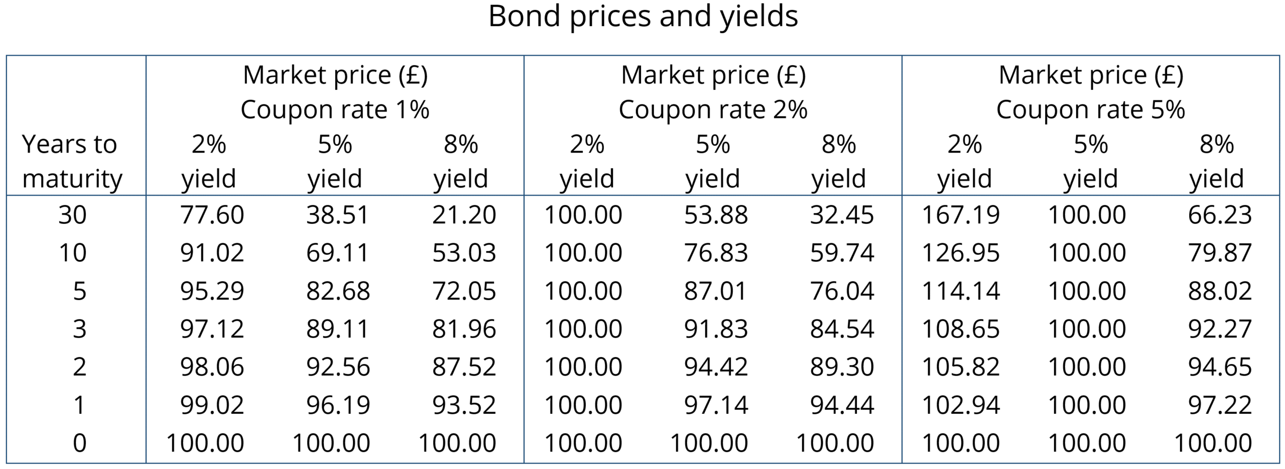
The higher the YTM, the lower the market price of a bond. Since the YTM reflects in part current rates of interest, so the higher the rate of interest, the lower the market price of any given bond. Thus bond yields vary directly with interest rates and bond prices vary inversely. You can see this clearly from the table. You can also see that market bond prices converge on the face value as the maturity date approaches.
Recent activity in bond markets
Investing in government bonds is regarded as very safe. Coupon payments are guaranteed, as is repayment of the face value on the maturity date. For this reason, many pension funds hold a lot of government bonds issued by financially trustworthy governments. But in recent months, bond prices in the secondary market have fallen substantially as interest rates have risen. For those holding existing bonds, this means that their value has fallen. For governments wishing to borrow by issuing new bonds, the cost has risen as they have to offer a higher coupon rate to attract buyers. This make it more expensive to finance government debt.
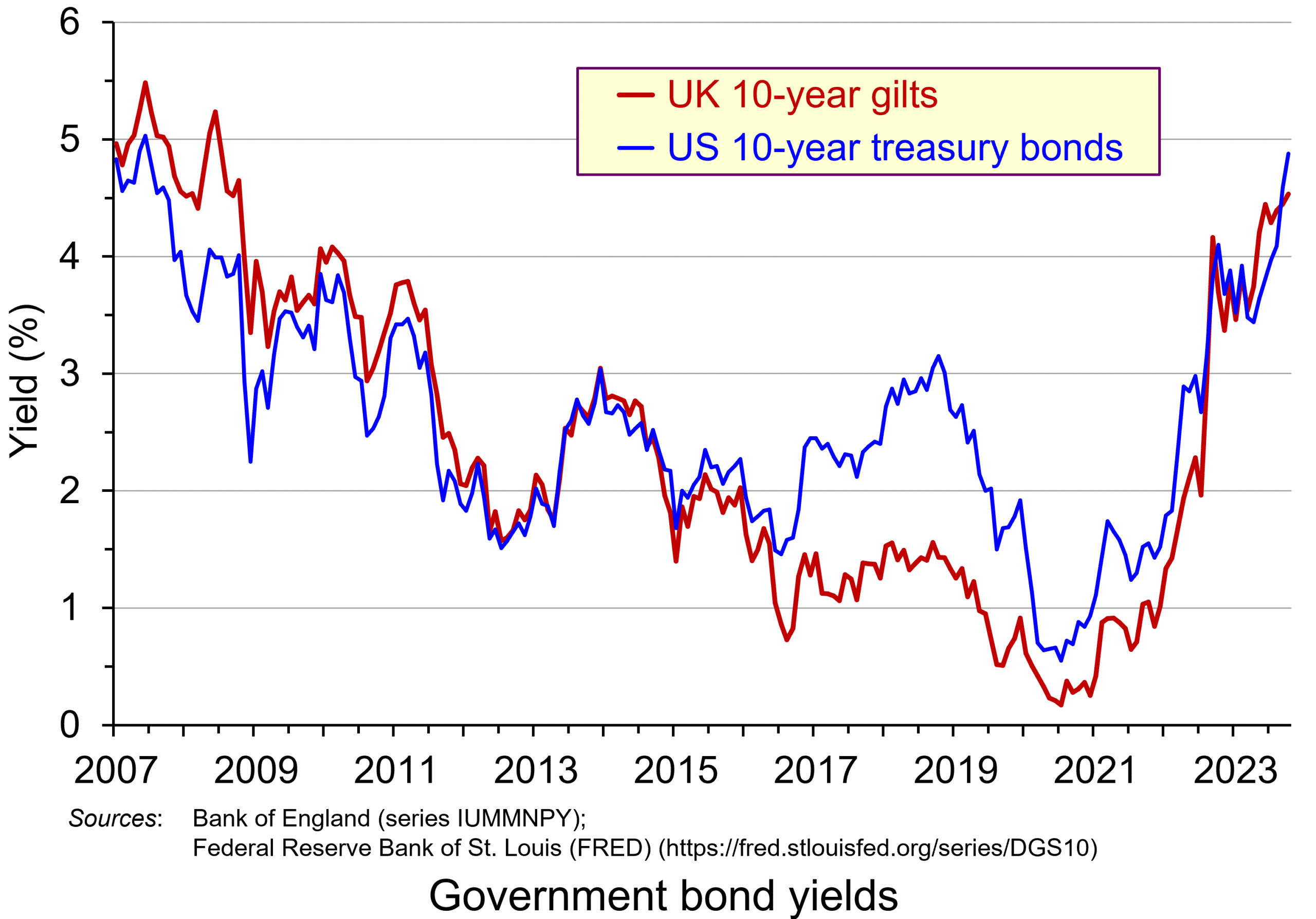 The chart shows the yield on 10-year government bonds. It is calculated using the ‘par value’ approach. This gives the coupon rate that would have to be paid for the market price of a bond to equal its face value. Clearly, as interest rates rise, a bond would have to pay a higher coupon rate for this to happen. (This, of course, is only hypothetical to give an estimate of market rates, as coupon rates are fixed at the time of a bond’s issue.)
Par values reflect both yield to maturity and also expectations of future interest rates. The higher people expect future interest rates to be, the higher must par values be to reflect this.
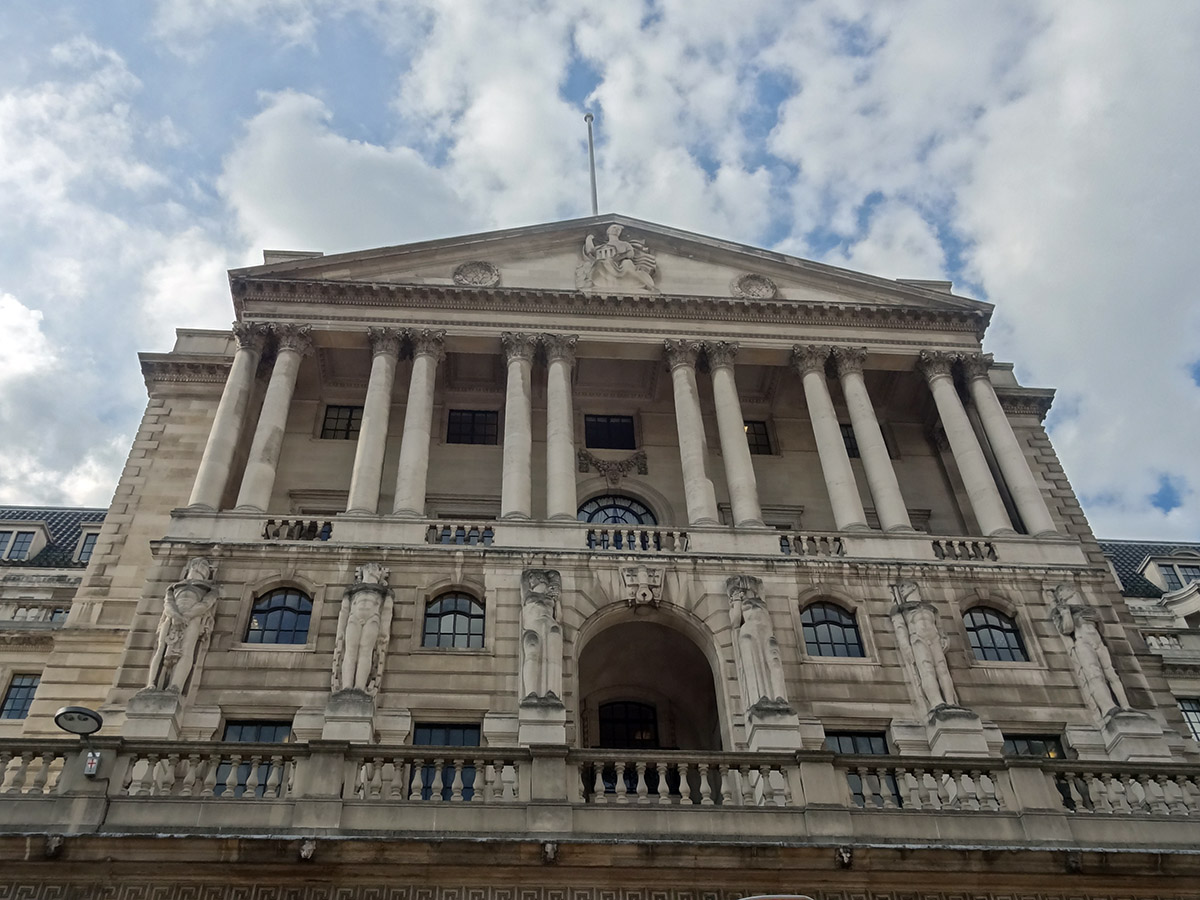 In the years following the financial crisis of 2007–8 and the subsequent recession, and again during the COVID pandemic, central banks cut interest rates and supported this by quantitative easing. This involved central banks buying existing bonds on the secondary market and paying for them with newly created (electronic) money. This drove up bond prices and drove down yields (as the chart shows). This helped support the policy of low interest rates. This was a boon to governments, which were able to borrow cheaply.
This has all changed. With quantitative tightening replacing quantitative easing, central banks have been engaging in asset sales, thereby driving down bond prices and driving up yields. Again, this can be seen in the chart. This has helped to support a policy of higher interest rates.
Problems of higher bond yields/lower bond prices
Although lower bond prices and higher yields have supported a tighter monetary policy, which has been used to fight inflation, this has created problems.
First, it has increased the cost of financing government debt. In 2007/8, UK public-sector net debt was £567bn (35.6% of GDP). The Office for Budget Responsibility forecasts that it will be £2702bn (103.1% of GDP in the current financial year – 2023/24). Not only, therefore, are coupon rates higher for new government borrowing, but the level of borrowing is now a much higher proportion of GDP. In 2020/21, central government debt interest payments were 1.2% of GDP; by 2022/23, they were 4.4% (excluding interest on gilts held in the Bank of England, under the Asset Purchase Facility (quantitative easing)).
 In the USA, there have been similar increases in government debt and debt interest payments. Debt has increased from $9tn in 2007 to $33.6tn today. Again, with higher interest rates, debt interest as a percentage of GDP has risen: from 1.5% of GDP in 2021 to a forecast 2.5% in 2023 and 3% in 2024. What is more, 31 per cent of US government bonds will mature next year and will need refinancing – at higher coupon rates.
There is a similar picture in other developed countries. Clearly, higher interest payments leave less government revenue for other purposes, such as health and education.
Second, many pension funds, banks and other investment companies hold large quantities of bonds. As their price falls, so this reduces the value of these companies’ assets and makes it harder to finance new purchases, or payments or loans to customers. However, the fact that new bonds pay higher interest rates means that when existing bond holdings mature, the money can be reinvested at higher rates.
Third, bonds are often used by companies as collateral against which to borrow and invest in new capital. As bond prices fall, this can hamper companies’ ability to invest, which will lead to lower economic growth.
Fourth, higher bond yields divert demand away from equities (shares). With equity markets falling back or at best ceasing to rise, this erodes the value of savings in equities and may make it harder for firms to finance investment through new issues.
At the core of all these problems is inflation and budget deficits. Central banks have responded by raising interest rates. This drives up bond yields and drives down bond prices. But bond prices and yields depend not just on current interest rates, but also on expectations about future interest rates. Expectations currently are that budget deficits will be slow to fall as governments seek to support their economies post-COVID. Also expectations are that inflation, even though it is falling, is not falling as fast as originally expected – a problem that could be exacerbated if global tensions increase as a result of the ongoing war in Ukraine, the Israel/Gaza war and possible increased tensions with China concerning disputes in the China Sea and over Taiwan. Greater risks drive up bond yields as investors demand a higher interest premium.
Articles
Information and data
Questions
- Why do bond prices and bond yields vary inversely?
- How are bond yields and prices affected by expectations?
- Why are ‘current yield’ and ‘yield to maturity’ different?
- What is likely to happen to bond prices and yields in the coming months? Explain your reasoning.
- What constraints do bond markets place on fiscal policy?
- Would it be desirable for central banks to pause their policy of quantitative tightening?
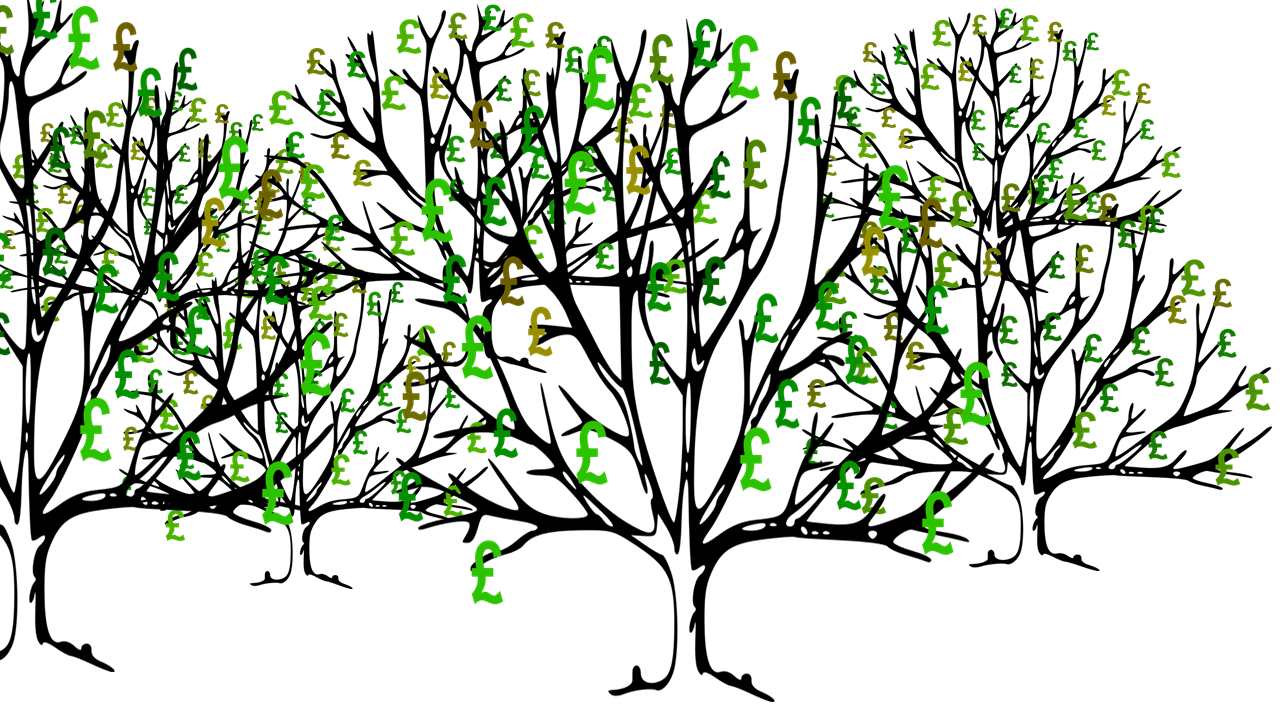 The BBC podcast linked below looks at the use of quantitative easing since 2009 and especially the most recent round since the onset of the pandemic.
Although QE was a major contributor to reducing the depth of the recession in 2009–10, it was barely used from 2013 to 2020 (except for a short period in late 2016/early 2017). The Coalition and Conservative governments were keen to get the deficit down. In justifying pay restraint and curbing government expenditure, Prime Ministers David Cameron and Theresa May both argued that there ‘was no magic money tree’.
But with the severely dampening effect of the lockdown measures from March 2020, the government embarked on a large round of expenditure, including the furlough scheme and support for businesses.
 The resulting rise in the budget deficit was accompanied by a new round of QE from the beginning of April. The stock of assets purchased by the Bank of England rose from £445 billion (the approximate level it had been since March 2017) to £740 billion by December 2020 and is planned to reach £895 billion by the end of 2021.
So with the effective funding of the government’s deficits by the creation of new money, does this mean that there is indeed a ‘magic money tree’ or, indeed, a ‘magic money forest’? And if so, is it desirable? Is it simply stoking up problems for the future? Or will, as modern monetary theorists maintain, the extra money, if carefully spent, lead to faster growth and a reducing deficit, with low interest rates making it easy to service the debt?
The podcast explores these issues. There is then a longer list of questions than normal relating to the topics raised in the podcast.
Podcast
Questions
- Which of the following are stocks and which are flows?
(a) Money
(b) Income
(c) The total amount people save each month
(d) The money held in savings accounts
(e) Public-sector net debt
(f) Public-sector net borrowing
(g) National income
(h) Injections into the circular flow of income
(i) Aggregate demand
(j) Wealth
- How do banks create money?
- What is the role of the Debt Management Office in the sale of gilts?
- Describe the birth of QE.
- Is raising asset prices the best means of stimulating the economy? What are the disadvantages of this form of monetary expansion?
- What are the possible exit routes from QE and what problems could occur from reducing the central bank’s stock of assets?
- Is the use of QE in the current Covid-19 crisis directly related to fiscal policy? Or is this use of monetary policy simply a means of hitting the inflation target?
- What are the disadvantages of having interest rates at ultra-low levels?
- Does it matter if the stock of government debt rises substantially if the gilts are at ultra-low fixed interest rates?
- What are the intergenerational effects of substantial QE? Does it depend on how debt is financed?
- How do the policy recommendations of modern monetary theorists differ from those of more conventional macroeconomists?
- In an era of ultra-low interest rates, does fiscal policy have a greater role to play than monetary policy?
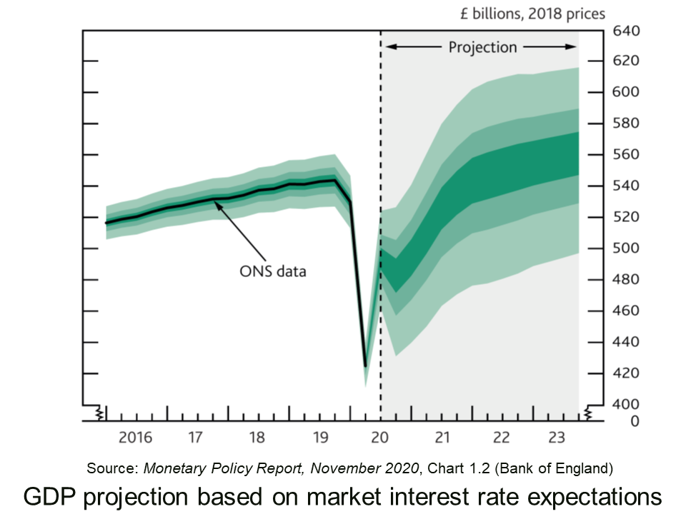
 With the imposition of a new lockdown in England from 5 November to 2 December and in Wales from 3 October to 9 November, and with strong restrictions in Scotland and Northern Ireland, the UK economy is set to return to negative growth – a W-shaped GDP growth curve.
With the closure of leisure facilities and non-essential shops in England and Wales, spending is likely to fall. Without support, many businesses would fail and potential output would fall. In terms of aggregate demand and supply, both would decline, as the diagram below illustrates. (Click here for a PowerPoint.)
The aggregate demand curve shifts from AD1 to AD2 as consumption and investment fall. Exports also fall as demand is hit by the pandemic in other countries. 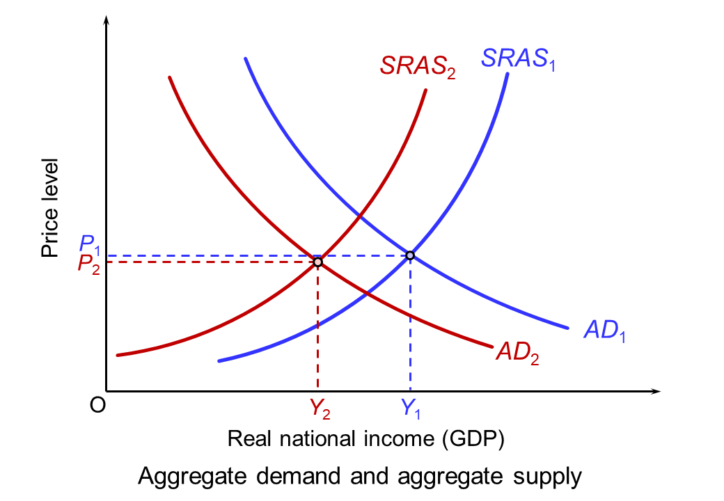 The fall in aggregate supply is represented partly by a movement along the short-run aggregate supply curve (SRAS) as demand falls for businesses which remain open (such as transport services). Largely it is represented by a leftward shift in the curve from SRAS1 to SRAS2 as businesses such as non-essential shops and those in the hospitality and leisure sector are forced to close. What happens to the long-run supply curve depends on the extent to which businesses reopen when the lockdown and any other subsequent restrictions preventing their reopening are over. It also depends on the extent to which other firms spring up or existing firms grow to replace the business of those that have closed. The continuing rise in online retailing is an example.
With the prospect of falling GDP and rising unemployment, the UK government and the Bank of England have responded by giving a fiscal and monetary boost. We examine each in turn.
Fiscal policy
 In March, the Chancellor introduced the furlough scheme, whereby employees temporarily laid off would receive 80% of their wages through a government grant to their employers. This scheme was due to end on 31 October, to be replaced by the less generous Job Support Scheme (see the blog, The new UK Job Support Scheme: how much will it slow the rise in unemployment?). However, the Chancellor first announced that the original furlough scheme would be extended until 2 December for England and then, on 5 November, to the end of March 2021 for the whole of the UK. He also announced that the self-employed income support grant would increase from 55% to 80% of average profits up to £7500.
In addition, the government announced cash grants of up to £3000 per month for businesses which are closed (worth more than £1 billion per month), extra money to local authorities to support businesses and an extension of existing loan schemes for business. Furthermore, the government is extending the scheme whereby people can claim a repayment ‘holiday’ for up to 6 months for mortgages, personal loans and car finance.
The government hopes that the boost to aggregate demand will help to slow, or even reverse, the predicted decline in GDP. What is more, by people being put on furlough rather than being laid off, it hopes to slow the rise in unemployment.
Monetary policy
At the meeting of the Bank of England’s Monetary Policy Committee on 4 November, further expansionary monetary policy was announced. Rather than lowering Bank Rate from its current historically low rate of 0.1%, perhaps to a negative figure, it was decided to engage in further quantitative easing.
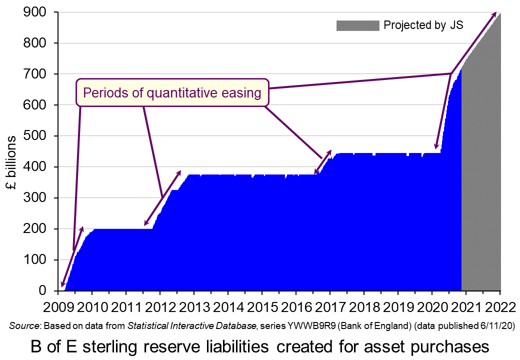 An additional £150 billion of government bonds will be purchased under the asset purchase facility (APF). This will bring the total vale of bonds purchased since the start of the pandemic to £450 billion (including £20 billion of corporate bonds) and to £895 billion since 2009 when QE was first introduced in response to the recession following the financial crisis of 2007–8.
The existing programme of asset purchases should be complete by the end of December this year. The Bank of England expects the additional £150 billion of purchases to begin in January 2021 and be completed within a year.
UK quantitative easing since the first round in March 2009 is shown in the chart above. The reserve liabilities represent the newly created money for the purchase of assets under the APF programme. (There are approximately £30 billion of other reserve liabilities outside the APF programme.) The grey area shows projected reserve liabilities to the end of the newly announced programme of purchases, by which time, as stated above, the total will be £895 billion. This, of course, assumes that the Bank does not announce any further QE, which it could well do if the recovery falters.

Justifying the decision, the MPC meeting’s minutes state that:
There are signs that consumer spending has softened across a range of high-frequency indicators, while investment intentions have remained weak. …The fall in activity over 2020 has reflected a decline in both demand and supply. Overall, there is judged to be a material amount of spare capacity in the economy.
Conclusions
How effective these fiscal and monetary policy measures will be in mitigating the effects of the Covid restrictions remains to be seen. A lot will depend on how successful the lockdown and other restrictions are in slowing the virus, how quickly a vaccine is developed and deployed, whether a Brexit deal is secured, and the confidence of both consumers, businesses and financial markets that the economy will bounce back in 2021. As the MPC’s minutes state:
The outlook for the economy remains unusually uncertain. It depends on the evolution of the pandemic and measures taken to protect public health, as well as the nature of, and transition to, the new trading arrangements between the European Union and the United Kingdom. It also depends on the responses of households, businesses and financial markets to these developments.
Articles
- Covid: Rishi Sunak to extend furlough scheme to end of March
BBC News (6/11/20)
- Furlough extended until March and self-employed support boosted again
MSE News, Callum Mason (6/11/20)
- Number on furlough in UK may double during England lockdown
The Guardian, Richard Partington (3/11/20)
- ‘We wouldn’t manage without it’: business owners on the furlough extension
The Guardian, Molly Blackall and Mattha Busby (6/11/20)
- Sunak’s abrupt turn on UK furlough scheme draws criticism from sceptics
Financial Times, Delphine Strauss (6/11/20)
 Coronavirus: Bank of England unleashes further £150bn of support for economy
Sky News, James Sillars (5/11/20)
- Bank of England boss pledges to do ‘everything we can’
BBC News, Szu Ping Chan (6/11/20)
- Savers are spared negative rates but the magic money tree delivers £150bn more QE: What the Bank of England’s charts tell us about the economy
This is Money, Simon Lambert (5/11/20)
- Covid-19 and the victory of quantitative easing
The Spectator, Bruce Anderson (26/10/20)
- Will the Bank of England’s reliance on quantitative easing work for the UK economy?
The Conversation, Ghulam Sorwar (9/11/20)
- With a W-shaped recession looming and debt piling up, the government should start issuing GDP-linked bonds
LSE British Politics and Policy blogs, Costas Milas (6/11/20)
Official documents
Questions
- Illustrate the effects of expansionary fiscal and monetary policy on (a) a short-run aggregate supply and demand diagram; (b) a long-run aggregate supply and demand diagram.
- In the context of the fiscal and monetary policy measures examined in this blog, what will determine the amount that the curves shift?
- Illustrate on a Keynesian 45° line diagram the effects of (a) the lockdown and (b) the fiscal and monetary policy measures adopted by the government and Bank of England.
- If people move from full-time to part-time working, how is this reflected in the unemployment statistics? What is this type of unemployment called?
- How does quantitative easing through asset purchases work through the economy to affect output and employment? In other words, what is the transmission mechanism of the policy?
- What determines the effectiveness of quantitative easing?
- Under what circumstances will increasing the money supply affect (a) real output and (b) prices alone?
- Why might quantitative easing benefit the rich more than the poor?
- How could the government use quantitative easing to finance its budget deficit?
After the November 2009 meeting of the Monetary Policy Committee, the Bank of England announced that it would keep Bank Rate on hold at 0.5%, at which rate it has been since March. It also said that it would spend a further £25 billion over the next three months on asset purchases, primarily government bonds, thereby pumping additional money into the economy: the process known as “quantitative easing“. This would bring total asset purchases under the scheme to £200bn.
But although this represents a further increase in money supply, the rate of increase is slowing down. In the previous three months, £50 billion of assets had been purchased. So does this imply that the Bank of England sees a recovery around the corner? Will money supply have been expanded enough to finance the desired increase in spending – on both consumption and investment?
A problem so far is that most of the extra money has not been spent on goods and services. Banks have been building up their reserves, with much of the money simply being re-deposited in the Bank of England as reserve balances (see Table A1.1.1 in “Bankstats). At the same time, households have been taking on very little extra debt – indeed, In July, total household debt actually fell (see “Payback time) and consumer debt (i.e. excluding mortgages) has continued to fall. If quantitative easing is to work, the money must be spent!
But with the monetary base having expanded so much, is there a danger that, once the recovery gathers pace, spending growth will return with a vengeance? Will inflation rapidly become a problem again with an overheating economy? The following articles examine the issues.
Interest rates held at 0.5 per cent (includes video) Channel 4 News (5/11/09)
Bank of England extends quantitative easing to £200bn Guardian, Larry Elliott (5/11/09)
What the economists say: Quantitative easing £25bn boost Guardian (5/11/09)
Bank of England faced with its biggest split on policy in a decade Independent, Sean O’Grady (4/11/09)
Bank of England expands money-printing programme to £200bn to fight downturn (includes video) Telegraph (5/11/09)
The one thing worse than quantitative easing would be no QE at all Telegraph, Edmund Conway (5/11/09)
BoE: It ain’t over till it’s over Telegraph, Edmund Conway blog (5/11/09)
Bank raises stimulus to £200bn to end recession Times Online, Grainne Gilmore (5/11/09)
Bank of England to inject another £25bn of stimulus money Management Today (5/11/09)
Extra £25bn to stimulate economy BBC News (5/11/09)
Quantitative easing ‘not working’ (video of DeAnne Julius: former MPC member) BBC News (5/11/09)
Boxed in BBC Stephanomics (5/11/09)
The BoE’s £25bn gambit Financial Times, Chris Giles blog (5/11/09)
US to reduce Quantitative Easing as rates kept low Telegraph, James Quinn (4/11/09)
 Quantitative easing ‘unpleasant’ BBC Today Programme, Stephen Bell and Wilem Buiter (7/11/09)
Experts debate whether quantitative easing is working (video) BBC Newsnight (6/11/09)
Questions
- What has been happening to the velocity of circulation of (narrow) money in the past few months? Explain the significance of this.
- What is likely to happen to the velocity of circulation in the coming months if (a) the economy recovers quite strongly; (b) recovery is modest?
- What is the relationship between quantitative easing and the growth in broad money (i.e. M4 in the UK)? How will banks’ desire to build up their reserves affect this relationship?
- Is the UK economy in a liquidity trap? Explain.
- Why is it likely that the Bank of England may well engage in more quantitative easing next March and beyond? How is the fiscal situation likely to affect Bank of England decisions?
- Examine the argument for the Bank of England buying more private-sector debt (virtually all of the asset purchases have been of public-sector debt)?
 To finance budget deficits, governments have to borrow. They can borrow short-term by issuing Treasury bills, typically for 1, 3 or 6 months. These do not earn interest and hence are sold at a discount below the face value. The rate of discount depends on supply and demand and will reflect short-term market rates of interest. Alternatively, governments can borrow long-term by issuing bonds. In the UK, these government securities are known as ‘gilts’ or ‘gilt-edged securities’. In the USA they are known as ‘treasury bonds’, ‘T-bonds’ or simply ‘treasuries’. In the EU, countries separately issue bonds but the European Commission also issues bonds.
![]()
 Bonds can be sold on the secondary market (i.e. the stock market) before maturity. The market price, however, is unlikely to be the coupon price (i.e. the face value). The lower the coupon rate relative to current interest rates, the less valuable the bond will be. For example, if interest rates rise, and hence new bonds pay a higher coupon rate, the market price of existing bonds paying a lower coupon rate must fall. Thus bond prices vary inversely with interest rates.
![]()


 The chart shows the yield on 10-year government bonds. It is calculated using the ‘par value’ approach. This gives the coupon rate that would have to be paid for the market price of a bond to equal its face value. Clearly, as interest rates rise, a bond would have to pay a higher coupon rate for this to happen. (This, of course, is only hypothetical to give an estimate of market rates, as coupon rates are fixed at the time of a bond’s issue.)
  In the years following the financial crisis of 2007–8 and the subsequent recession, and again during the COVID pandemic, central banks cut interest rates and supported this by quantitative easing. This involved central banks buying existing bonds on the secondary market and paying for them with newly created (electronic) money. This drove up bond prices and drove down yields (as the chart shows). This helped support the policy of low interest rates. This was a boon to governments, which were able to borrow cheaply.
 In the USA, there have been similar increases in government debt and debt interest payments. Debt has increased from $9tn in 2007 to $33.6tn today. Again, with higher interest rates, debt interest as a percentage of GDP has risen: from 1.5% of GDP in 2021 to a forecast 2.5% in 2023 and 3% in 2024. What is more, 31 per cent of US government bonds will mature next year and will need refinancing – at higher coupon rates.
 The BBC podcast linked below looks at the use of quantitative easing since 2009 and especially the most recent round since the onset of the pandemic.
  The resulting
 With the imposition of a new lockdown in England from 5 November to 2 December and in Wales from 3 October to 9 November, and with strong restrictions in Scotland and Northern Ireland, the UK economy is set to return to negative growth – a W-shaped GDP growth curve.
  The fall in aggregate supply is represented partly by a movement along the short-run aggregate supply curve (SRAS) as demand falls for businesses which remain open (such as transport services). Largely it is represented by a leftward shift in the curve from SRAS1 to SRAS2 as businesses such as non-essential shops and those in the hospitality and leisure sector are forced to close. What happens to the long-run supply curve depends on the extent to which businesses reopen when the lockdown and any other subsequent restrictions preventing their reopening are over. It also depends on the extent to which other firms spring up or existing firms grow to replace the business of those that have closed. The continuing rise in online retailing is an example.
 In March, the Chancellor introduced the furlough scheme, whereby employees temporarily laid off would receive 80% of their wages through a government grant to their employers. This scheme was due to end on 31 October, to be replaced by the less generous Job Support Scheme (see the blog,
  An additional £150 billion of government bonds will be purchased under the asset purchase facility (APF). This will bring the total vale of bonds purchased since the start of the pandemic to £450 billion (including £20 billion of corporate bonds) and to £895 billion since 2009 when QE was first introduced in response to the recession following the financial crisis of 2007–8.