Large European banks call for further integration, but is it in consumers’ interests?
 Those of a certain age may remember the fanfare which heralded the introduction of the Single European market (SEM) on 1 January 1993. It promised the removal of internal barriers to the movement of goods, services, capital and people. One sector that was noticeably absent from the single market, however, was banking.
Moves towards banking union only started after the global financial crisis in 2008. However, as a report published on the 2 September 2025 by the Association of Financial Markets in Europe (AFME) highlights, the institutional frameworks of banking in the EU are still deeply fragmented – the promised integration through the European Banking Union (EBU) is still incomplete. This has put European banks at a competitive disadvantage in global markets compared with rivals from the USA and Asia, thereby reducing their profitability and growth prospects. The report called on the European Central Bank (ECB) and national regulatory authorities to remove hurdles to cross-border banking services in the EU. This would enhance the strategic position of European banks.
In this blog we will trace the development of the EBU and analyse the current state of integration. We discuss the AFME proposals for achieving greater integration and highlight their benefits for large banks. We also analyse the barriers which limit full integration and examine the risks that retail customers might see few benefits from the proposed changes.
What is meant by European Banking Union (EBU)?
The 1993 Single European Market (SEM) in goods and services removed internal barriers to the movement of goods, services, capital and people within the EU. As part of this, there were harmonised standards and regulations for goods and services, no capital controls, mutual recognition of professional qualifications and common regulations on consumer protection, product safety, environmental protection and labour rights.
This integration of previously restricted domestic markets was designed to boost economic growth, employment and competitiveness by increasing trade and investment flows. Offering consumers greater choice would expose firms to greater competition. This would drive down prices and encourage greater efficiency and innovation. It has generally achieved these goals across many industries.
However, banking was excluded from integration. The 1985 White Paper, Completing the Internal Market, proposed the liberalisation of financial services, but banking remained regulated at the national level. This was influenced by interrelated economic, political and institutional forces, national sovereignty and political sensitivities, fragmented regulation and concerns about risk.
 Even as the EU moved towards economic and monetary union (EMU) during the 1990s, there was no discussion of integration for the banking industry. However, that changed following the 2008 financial crisis and 2011 eurozone crisis. Both episodes exposed vulnerabilities in the EU banking system which required taxpayer support. It was proposed that deeper integration of the banking sector would ensure its stability and resilience. This stimulated moves towards European Banking Union (EBU), starting with the European Council agreeing its creation in 2012. There are three institutional pillars to the Union:
- The Single Supervisory Mechanism (2014) for systemically important financial institutions (SIFIs) ensures consistent oversight. SIFIs are banks with over €30 billion of liabilities or 20% of national GDP.
- The Single Resolution Mechanism (2016) manages the orderly resolution of failing banks with minimal costs to taxpayers. There is a central board for resolution decisions and a fund financed by the banking industry to support resolution actions.
- A European Deposit Insurance Scheme (still under negotiation) is proposed to protect depositors uniformly across the banking union against bank default.
The Union is intended to operate under a harmonised set of EU laws, known as the ‘Single Rulebook’, which includes implementing the BASEL III capital requirements, regulating national deposit insurance and setting rules for managing failing banks.
What is the state of integration at present?
Moves towards European Banking Union (EBU) have contributed to enhancing the resilience of the European banking system. This was one of its major objectives. European banks are much more secure having increased capital and liquidity levels, reduced credit risks and become less reliant on state-aid. They are also less profitable.
The AFME report points to remaining gaps in Banking Union which raise the cost for banks offering cross-border retail banking within the EU and limit the incentive to do so. The report identifies four such gaps.
 1. Ring fencing. Although there is a single supervisory mechanism for large systemically important institutions, since the financial crisis national regulators have implemented ‘ring-fencing’. This aims to protect retail banking activities from riskier investment banking. Ring-fencing retains liquidity, dividends and other bank assets within national borders to protect their retail banking sectors from contagion. The ECB estimates €225 billion of capital and €250 billion of liquidity is trapped by such national restrictions. Further, unharmonized and unpredictable use of capital buffers adds complexity for capital management at a multinational level. This particularly impacts large institutions. Banks’ cross-border activities are impeded since they are restricted in the way they can use capital and liquidity across the bloc.
The report argues that the stringent requirements of the ECB and the multiple layers of macroprudential requirements imposed at national level have led to an unnecessarily high level of capital. This disadvantages large European banks compared to their international competitors.
2. Impediments to cross-border M&As in banking within the EU. This is due to cumbersome authorisation processes, involving multiple authorities at both national and supra-national level. Further, national authorities may interfere in the process of M&As in a bid to prevent domestic banks being acquired by ones from other parts of the EU. A recent example is UniCredit’s bid for Germany’s Commerzbank, which the German government opposes. These characteristics restrict opportunities for consolidation and efficiency gains for European banks.
The AFME report estimates that once eurozone banks grow beyond €450 billion in total assets, they suffer from negative synergies putting them at a competitive disadvantage to global competitors. Indeed, US banks are able to leverage scale economies from their domestic market to enter large EU markets. An example is JP Morgan’s entry into multiple EU markets through its Chase brand.
3. Contributions to the Single Resolution Fund (SRF) are complex and lack transparency. This makes it difficult for banks to predict future commitments. The fund itself and its target level were determined at a time when banks had low buffers. Since then, European banks have raised their loss absorbing capacity and the AFME report proposes that further increases in contributions to the fund need to be carefully considered and reviewed.
4. The Deposit Guarantee Scheme remains unimplemented and there are still differences in national schemes. This situation creates uncertainty for banks, which would like the European scheme for large systemically important institutions to be implemented fully.
These AFME proposals focus on the aspects of banking union which benefit large European institutions in their strategic competition with global rivals. These aspects would create ‘European’ banks as opposed to ‘national’ ones. This would give them the scale to be ‘champions’ in global competition. In particular, the large banks want lower capital requirements and the relaxation of national ring-fencing for retail banking to allow them greater freedom to achieve scale and scope economies across the bloc.
To what extent this will benefit retail customers, however, is debateable.
Will retail banking customers benefit?
Retail banking across Europe remains deeply fragmented, with significant price differentials from country to country. The following table illustrates pricing differentials for two retail products – loans and mortgages – across a sample of EU countries for July 2025.
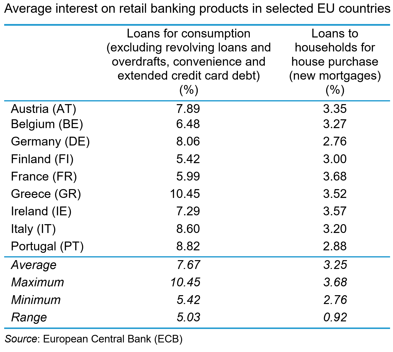
The data show a range of average interest rates offered across the countries with a range of 5.03% for loans to households and 0.92% for new mortgages. These price differentials reflect a broad array of factors, not least the different institutional legal and risk characteristics of the national markets. They also reflect varying degrees of competition and the lack of cross-border trade in retail banking products. Retail banking remains a largely domestic industry within the EU. Cross-border banking services remain a marginal activity with non-domestic retail deposits rising by just 0.5% and non-domestic retail loans rising by just 0.3% between 2016 and 2024.
There are both natural and policy-induced barriers, which means that retail banking will remain largely segmented by nation.
 On the demand-side, retail banking is largely a relational rather than a transactional service, with consumption taking place over a long time-period with significant financial risks attached. Even with deposit insurance and a lender of last resort (the central bank), consumers exhibit significant loss aversion in their use of retail banking services. Consequently, trust and confidence are important characteristics for consumers and that means they are likely to prefer to use familiar domestic institutions.
Further, perceptions about switching costs mean that consumers are reluctant to change suppliers. Such costs are exacerbated by language, cultural and legal differences between European countries, which can make the perceived costs of banking beyond national boundaries prohibitively expensive and create a preference for local institutions.
Consumer preferences can also create idiosyncratic market structures for retail banking services in particular countries. For instance, in several countries across the EU, notably Germany, mutualised credit unions account for significant shares of retail banking. This may limit the potential for foreign banks to penetrate Europe’s largest market.
There are also policy-induced obstacles to cross-border retail banking which operate on the demand-side. These include discriminatory tax treatment of foreign financial services which deters their purchase by consumers. Further, there are still eight different currencies used in the EU across the 27 member states (Denmark, Poland and Sweden are three significant examples). This creates costs and risks associated with currency exchange for consumers that may deter their use of cross-border deposits and loans. The full adoption of a single currency across the EU seems a long way off, which will limit the potential for a single banking market, particularly in the retail segment.
Retail banking as a public utility
 Some argue that retail banking is a public utility and should be regulated as such. It has a simple business model, taking deposits, making payments and making loans. Like other utilities, such as water and energy, retail banking is an essential service for the smooth functioning of the economy and society. Like other utilities, bank failures create severe problems for the economy and society.
Since the financial crisis, stability in retail banking has been much more highly valued. In the period preceding the crisis, banks had used retail deposits to cross-subsidise their risky investment banking. The bank failures that resulted from this had severe economic consequences. The danger today is that by relaxing capital and liquidity restrictions too much, large banks may once again engage in risky behaviour, subsidised by retail banking – for example, by engaging in cross-border M&As. These may benefit their shareholders but provide little benefit to retail customers.
Further, allowing these large banks freedom to move funds around the bloc may lead to capital being concentrated in the most profitable markets, leaving less profitable markets / countries underserved. Retail banking, as a public utility, should be required to provide services there.
Who ultimately benefits?
The integration of banking services in the EU has progressed since the financial crisis, producing a more resilient system. However, there are features of retail banking which mean that integration which benefits consumers may be difficult to achieve.
Addressing the policy gaps identified by the AFME report may benefit large European banks by facilitating the scale economies to make them competitive internationally. However, until consumers are prepared, or able, to source banking services beyond national borders, they will see little benefit from European Banking Union (EBU) through lower prices and/or better service. The nature of retail banking in the EU suggests that this is unlikely any time soon.
Furthermore, since retail banking exhibits features of a public utility, regulators need to be wary of permitting the type of behaviour by large institutions which creates dangerous systemic risk. The worry is that, in the drive to create ‘European Champions’ in banking, regulators ignore the potential impact on retail customers.
Articles
Book
Report
Data and Information
Questions
- Using an average cost (AC) schedule, illustrate the efficiency benefits for large European banks from banking union.
- Analyse the sources of efficiency gains that European banks can gain from cross-border M&As.
- Explain how European retail banking customers could gain from such efficiency.
- Analyse why they may not.
- Analyse whether retail banking in Europe needs to be regulated as a public utility.
 The UK’s poor record on productivity since the 2008 financial crisis is well documented, not least in this blog series. Output per worker has flatlined over the 17 years since the crisis. As was noted in the blog, The UK’s poor productivity record, low UK productivity is caused by a number of factors, including the lack of investment in training, the poor motivation of many workers and the feeling of being overworked, short-termism among politicians and management, and generally poor management practices.
One of the most significant issues identified by analysts and commentators is the lack of investment in physical capital, both by private companies and by the government in infrastructure. Gross fixed capital formation (a measure of investment) has been much lower in the UK compared to international competitors.
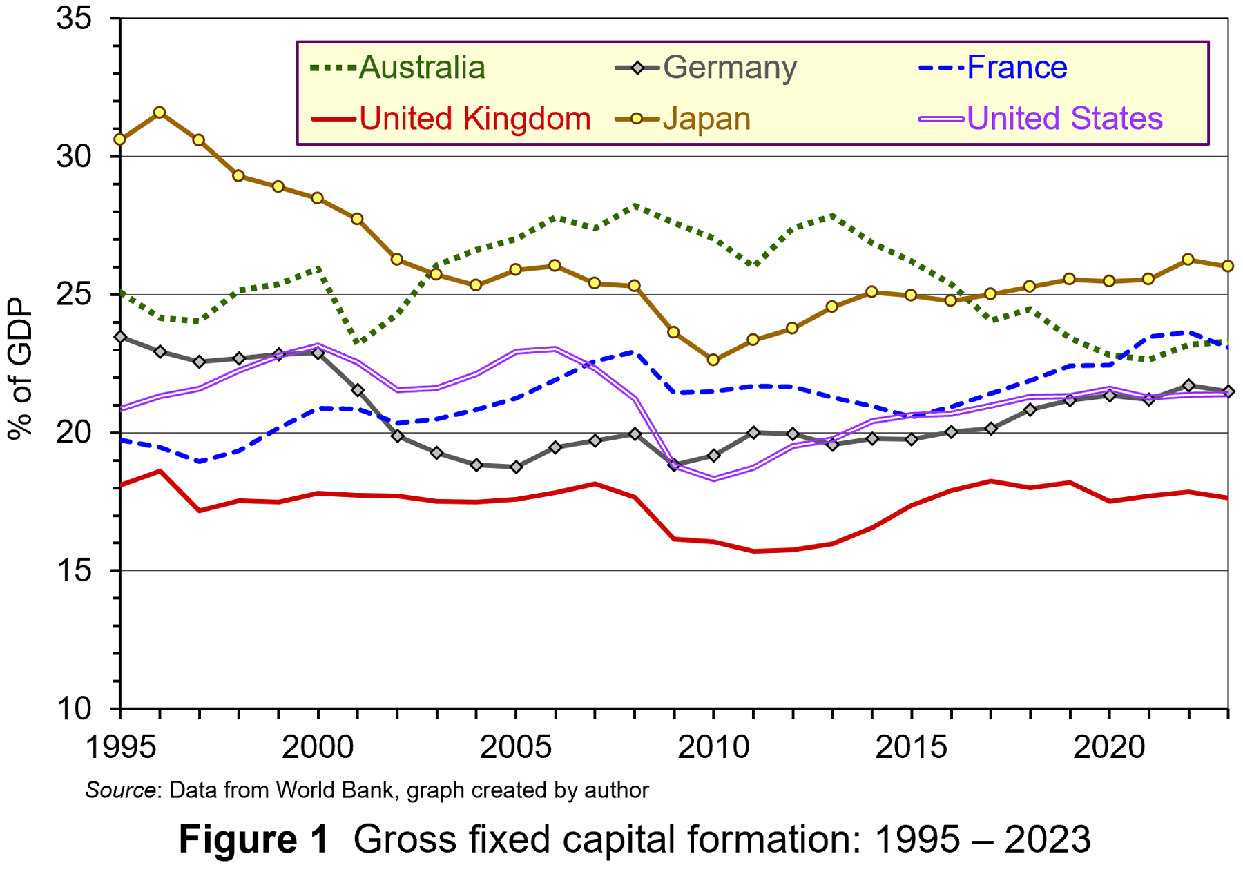 From Figure 1 it can be observed that, since the mid-1990s, the UK has consistently had lower investment as a percentage of GDP compared to other significant developed market economies. The cumulative effect of this gap has contributed to lower productivity and lower economic growth.
Interestingly, since the financial crisis, UK firms have had high profitability and associated high cash holdings. This suggests that firms have had a lot of financial resources to reinvest. However, data from the OECD suggests that reinvestment rates in the UK, typically 40–50% of profit, are much lower than in many other OECD countries. In the USA the rate is 50%, in Germany 60–70% and in Japan 70%+. There is much greater emphasis in the UK on returning funds to shareholders through dividends and share buybacks. However, the reinvestment of much of this cash within firms could have gone some way to addressing the UK’s investment gap – but, it hasn’t been done.
 Analysis by the OECD suggest that, while the cost of financing investment has declined since the financial crisis, the gap between this and the hurdle rate used to appraise investments has widened. Between 2010 and 2021 the difference nearly doubled to 4%. This increase in the hurdle rate can be related to increases in the expected rate of return by UK companies and their investors.
In this blog we will analyse (re)investment decisions by firms, discussing how increases in the expected rate of return in the UK raise the hurdle rate used to appraise investments. This reduces the incentive to engage in long-term investment. We also discuss policy prescriptions to improve reinvestment rates in the UK.
Investment and the expected rate of return
Investment involves the commitment of funds today to reap rewards in the future. This includes spending on tangible and intangible resources to improve the productive capacity of firms. Firms must decide whether the commitment of funds is worthwhile. To do so, economic theory suggests that they need to consider the compensation required by their provider of finance – namely, investors.
What rewards do investors require to keep their funds invested with the firm?
When conducting investment appraisal, firms compare the estimated rate of return from an investment with the minimum return investors are prepared to receive (termed the ‘expected return’). Normally this is expressed as a percentage of the initial outlay. Firms have to offer returns to investors which are equal to or greater than the minimum expected return – the return that is sufficient to keep funds invested in the firm. Therefore, returns above this minimum expected level are termed ‘excess returns’.
When firms conduct appraisals of potential investments, be it in tangible or intangible capital, they need to take into account the fact that net benefits, expressed as cash flows, will accrue over the life of the investment, not all at once. To do this, they use discounted cash flow (DCF) analysis. This converts future values of the net benefits to their present value. This is expressed as follows:

Where:
NPV = Net present value (discounted net cash flows);
K = Capital outlay (incurred at the present time);
C = Net cash flows (occur through the life of the investment project);
r = Minimum expected rate of return.
In this scenario, the investment involves an initial cash outlay (K), followed in subsequent periods by net cash inflows each period over the life of the investment, which in this case is 25 years. All the cash flows are discounted back to the present so that they can be compared at the same point in time.
The discount rate (r) used in appraisals to determine the present value of net cash flows is determined by the minimum expected return demanded by investors. If at that hurdle rate there are positive net cash flows (+NPV), the investment is worthwhile and should be pursued. Conversely, if at that hurdle rate there are negative net cash flows (–NPV), the investment is not worthwhile and should not be pursued.
According to economic theory, if a firm cannot find any investment projects that produce a positive NPV, and therefore satisfy the minimum expected return, it should return funds to shareholders through dividends or share buybacks so that they can invest the finance more productively.
Firm-level data from the OECD suggest that UK firms have had higher profits and this has been associated with increased cash holdings. But, due to the higher hurdle rate, less investment is perceived to be viable and thus firms distribute more of their profits through dividends and share buybacks. These payouts represent lost potential investment and cumulatively produce a significant dent in the potential output of the UK economy.
Why are expected rates of return higher in the UK?
This higher minimum rate of expected return can be explained by factors influencing its determinants; opportunity cost and risk/uncertainty.
Higher opportunity cost. Opportunity cost relates to the rate of return offered by alternatives. Investors and, by implication firms, will have to consider the rate of return offered by alternative investment opportunities. Typically, investors have focused on interest rates as a measure of opportunity cost. Higher interest rates raise the opportunity cost of an investment and increase the minimum expected rate of return (and vice versa with lower interest rates).
 However, it is not interest rates that have increased the opportunity cost, and hence the minimum expected rate of return associated with investment, in the UK since the financial crisis. For most of the period since 2008, interest rates have been extremely low, sitting at below 1%, only rising significantly during the post-pandemic inflationary surge in 2022. This indicates that this source of opportunity cost for the commitment of business investment has been extremely low.
However, there may be alternative sources of opportunity cost which are pushing up the expected rate of return. UK investors are not restricted to investing in the UK and can move their funds between international markets determined by the rate of return offered. The following table illustrates the returns (in terms of percentage stock market index gain) from investing in a sample of UK, US, French and German stock markets between August 2010 and August 2025.
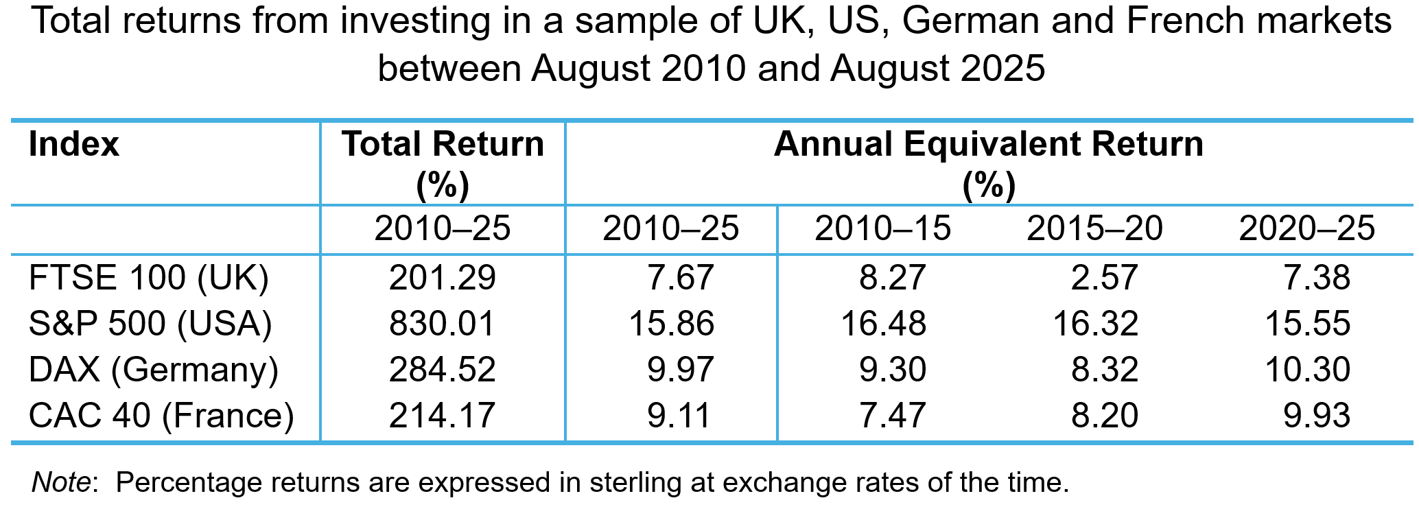
When expressed in sterling, returns offered by UK-listed companies are lower across the whole period and in most of the five-yearly sub-periods. Indeed, the annual equivalent rate of return (AER) for the FTSE 100 index across the whole period is less than half that of the S&P 500. The index offered a paltry annual return of 2.57% between 2015 and 2020, while the US index offered a return of 16.48%. Both the French and German indices offered higher rates of return, in the latter part of the period particularly. This represents a higher opportunity cost for UK investors and may have increased their expectations about the return they require for UK investments.
Greater perceived risk/uncertainty. Expected rates of return are also determined by perceptions of risk and uncertainty – the compensation investors need to bear the perceived risk associated with an investment. Investors are risk averse. They demand higher expected return as compensation for higher perceived risk. Higher levels of risk aversion increase the expected rate of return and related investment hurdle rates.
 There has been much discussion of increased uncertainty and risk aversion among global investors and firms (see the blogs Rising global uncertainty and its effects, World Uncertainty Index, The Chancellor’s fiscal dilemma and Investment set to fall as business is baffled by Trump). The COVID-19 pandemic, inflation shocks, the war in Ukraine, events across the Middle East and the trade policies adopted by the USA in 2025 have combined to produce a very uncertain business environment.
While these have been relatively recent factors influencing world-wide business uncertainty, perceptions of risk and uncertainty concerning the UK economy seem to be longer established. To measure policy-related economic uncertainty in the UK, Baker, Bloom and Davis at www.PolicyUncertainty.com construct an index based on the content analysis of newspaper articles mentioning terms reflecting policy uncertainty.
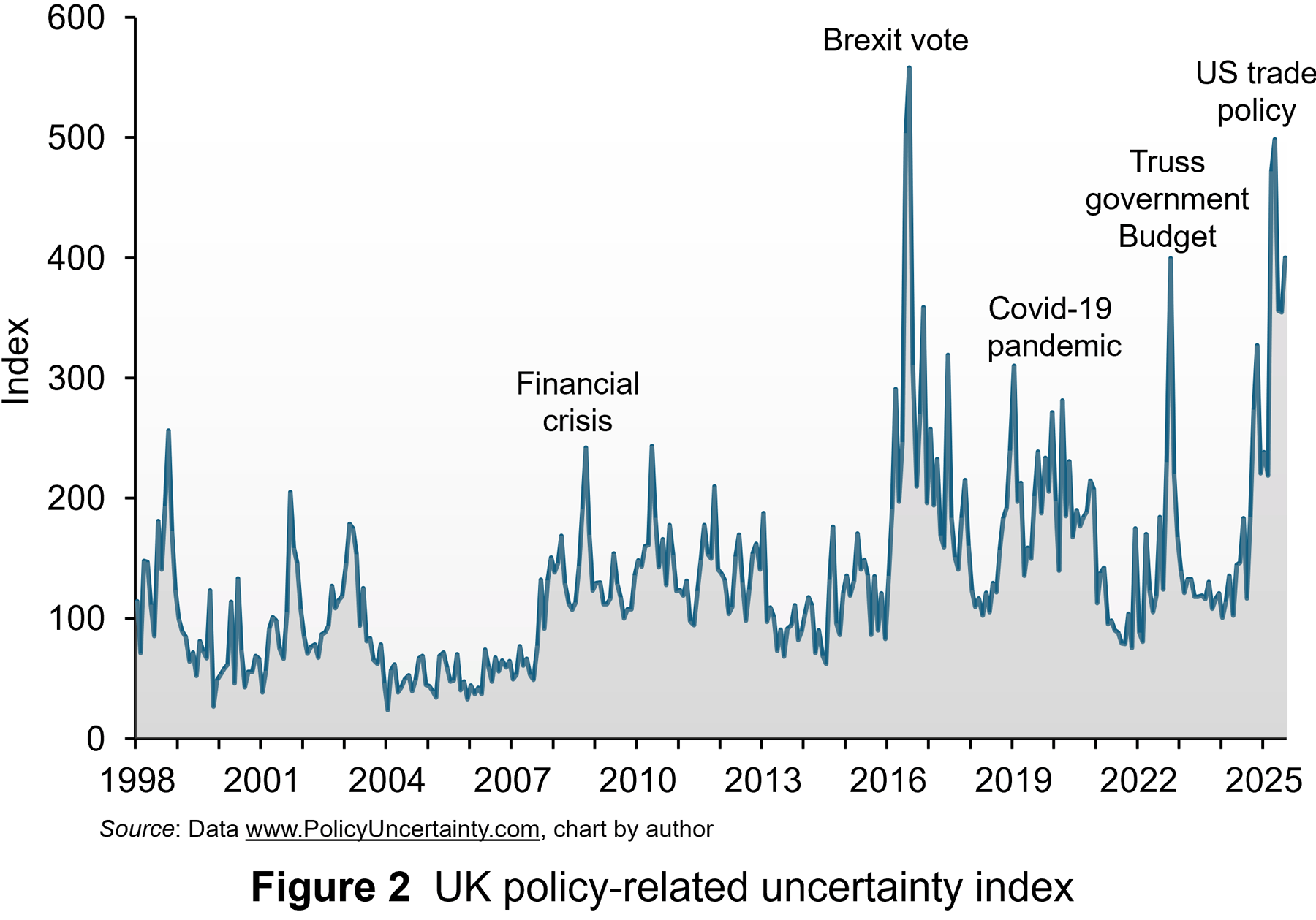 Figure 2 illustrates the monthly index from 1998 to July 2025. The series is normalised to standard deviation 1 prior to 2011 and then summed across papers, by month. Then, the series is normalised to mean 100 prior to 2011.
Some of the notable spikes in uncertainty in the UK since 2008 have been labelled. Beginning with the global financial crisis, investors and firms became much more uncertain. This was exacerbated by a series of economic shocks that hit the economy, one of which, the narrow vote to leave the European Union in 2016, was specific to the UK. This led to political turmoil and protracted negotiations over the terms of the trade deal after the UK left. This uncertainty has been exacerbated recently by the series of global shocks highlighted above and also the budget uncertainty of Liz Truss’s short-lived premiership and now the growing pressure to reduce government borrowing.
While spikes in uncertainty occurred before the financial crises, the average level of uncertainty, as measured by the index, has been much higher since the crisis. From 1998 to 2008, the average value was 89. Since 2008, the average value has been 163. Since the Brexit vote, the average value has been 185. This indicates a much higher perception of risk and uncertainty over the past 15 year and this translates into higher minimum expected return as compensation. Consequently, this makes many long-term investment projects less viable because of higher hurdle rates. This produces less productive investment in capital, contributing significantly to lower productivity.
Policy proposals
There has been much debate in the UK about promoting greater long-term investment. Reforms have been proposed to improve public participation in long-term investment through the stock market. To boost investment, this would require the investing public to be prepared to accept lower expected returns for a given level of risk or accept higher risk for a given level of returns.
Evidence suggests that the appetite for this may be very low. UK savers tend to favour less risky and more liquid cash deposits. It may be difficult to encourage them to accept higher levels of risk. In any case, even if they did, many may invest outside the UK where the risk-return trade-off is more favourable.
 Over the past 10 years, policy uncertainty has played a significant role in deterring investment. So, if there is greater continuity, this may then promote higher levels of investment.
The Labour government has proposed policies which aim to share or reduce the risk/uncertainty around long-term investment for UK businesses. For instance, a National Wealth Fund (NWF) has been established to finance strategic investment in areas such as clean energy, gigafactories and carbon capture. Unfortunately, the Fund is financed by borrowing through financial markets and the amount expected to be committed over the life of the current Parliament is only £29 billion, assuming that private capital matches public commitments in the ratio expected. It is questionable whether the Fund’s commitment will be sufficient to attract private capital.
Alternatively, Invest 2035 is a proposal to create a stable, long-term policy environment for business investment. It aims to establish an Industrial Strategy Council for policy continuity and to tackle issues like improving infrastructure, reducing energy costs and addressing skills gaps. Unfortunately, even if there is some attempt at domestic policy stability, the benefits may be more than offset by perceptions around global uncertainty, which may mean that UK investors’ minimum expected rates of return remain high and long-term investment low for the foreseeable future.
Articles
Data
Questions
- Use the marginal efficiency of capital framework to illustrate the ‘lost’ investment spending in the UK due to the investment hurdle rate being higher than the cost of capital.
- Explain the arbitrage process which produces the differences in valuations of UK securities and foreign ones due to differences in the expected rate of return.
- Sketch an indifference curve for a risk-averse investor, treating expected return and risk as two characteristics of a financial instrument.
- How does higher uncertainty affect the slope of an indifference curve for such an investor? How does this affect their investment hurdle rate?
- Analyse the extent to which the proposed polices can reduce the investment hurdle rate for UK companies and encourage greater levels of investment.
 We continue to live through incredibly turbulent times. In the past decade or so we have experienced a global financial crisis, a global health emergency, seen the UK’s departure from the European Union, and witnessed increasing levels of geopolitical tension and conflict. Add to this the effects from the climate emergency and it easy to see why the issue of economic uncertainty is so important when thinking about a country’s economic prospects.
In this blog we consider how we can capture this uncertainty through a World Uncertainty Index and the ways by which economic uncertainty impacts on the macroeconomic environment.
World Uncertainty Index
Hites Ahir, Nicholas Bloom and Davide Furceri have constructed a measure of uncertainty known as the World Uncertainty Index (WUI). This tracks uncertainty around the world using the process of ‘text mining’ the country reports produced by the Economist Intelligence Unit. The words searched for are ‘uncertain’, ‘uncertainty’ and ‘uncertainties’ and a tally is recorded based on the number of times they occur per 1000 words of text. To produce the index this figure is then multiplied up by 100 000. A higher number therefore indicates a greater level of uncertainty. For more information on the construction of the index see the 2022 article by Ahir, Bloom and Furceri linked below.
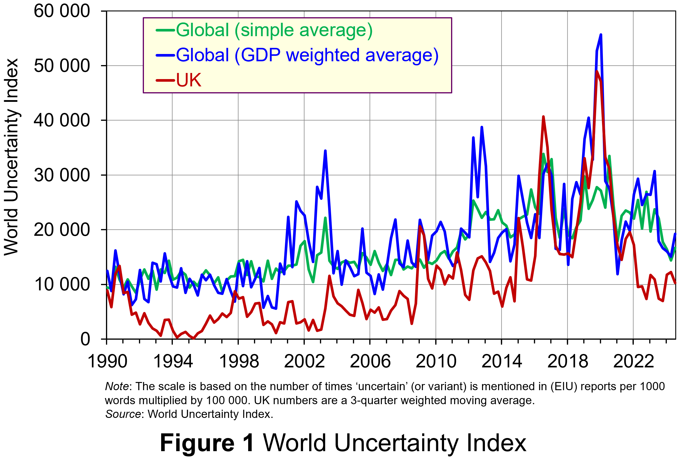 Figure 1 (click here for a PowerPoint) shows the WUI both globally and in the UK quarterly since 1991. The global index covers 143 countries and is presented as both a simple average and a GDP weighted average. The UK WUI is also shown. This is a three-quarter weighted average, the authors’ preferred measure for individual countries, where increasing weights of 0.1, 0.3 and 0.6 are used for the three most recent quarters.
From Figure 1 we can see how the level of uncertainty has been particularly volatile over the past decade or more. Events such as the sovereign debt crisis in parts of Europe in the early 2010s, the Brexit referendum in 2016, the COVID-pandemic in 2020–21 and the invasion of Ukraine in 2022 all played their part in affecting uncertainty domestically and internationally.
Uncertainty, risk-aversion and aggregate demand
Now the question turns to how uncertainty affects economies. One way of addressing this is to think about ways in which uncertainty affects the choices that people and businesses make. In doing so, we could think about the impact of uncertainty on components of aggregate demand, such as household consumption and investment, or capital expenditures by firms.
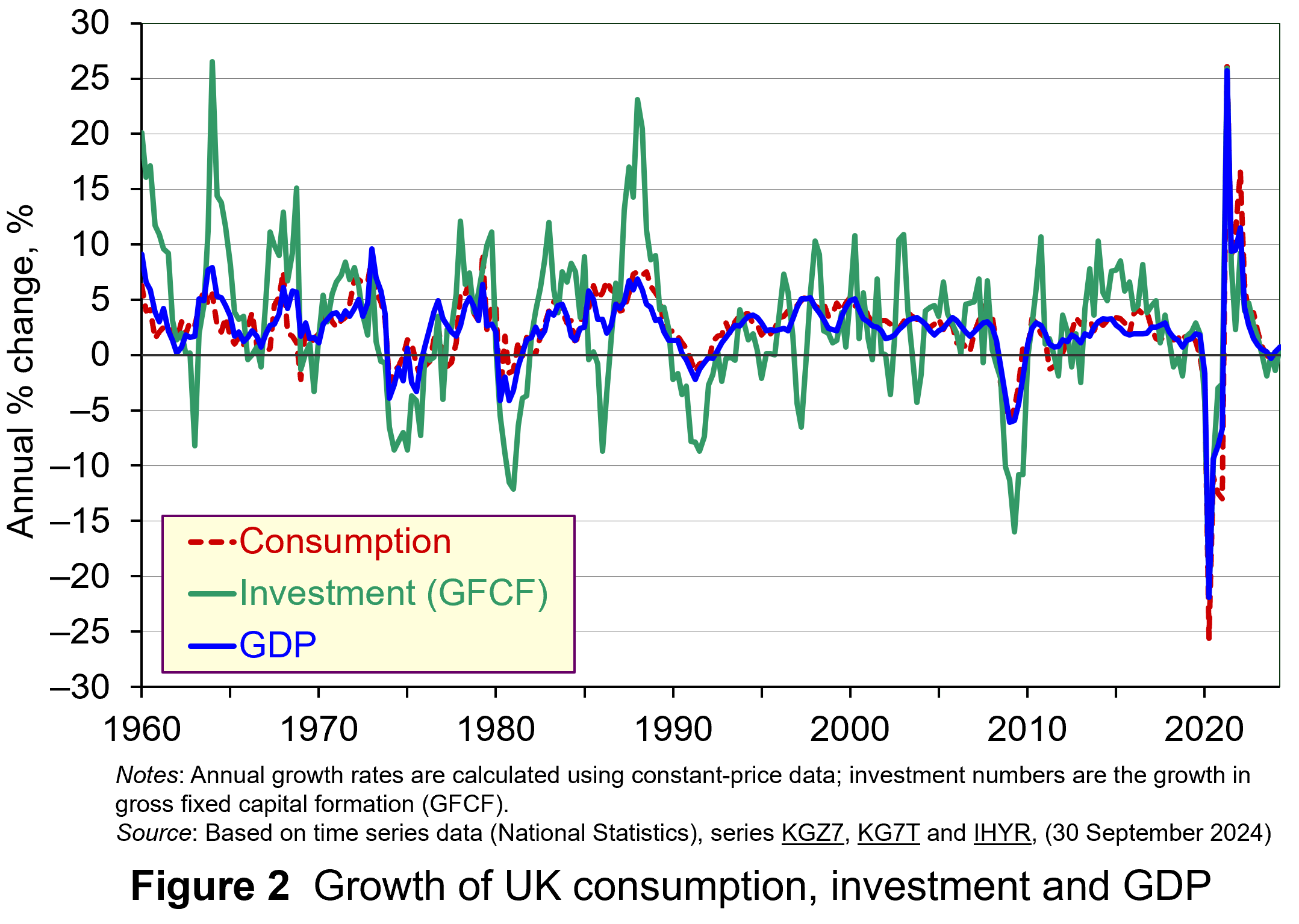 As Figure 2 shows (click here for a PowerPoint), investment is particularly volatile, and much more so than household spending. Some of this can be attributed to the ‘lumpiness’ of investment decisions since these expenditures tend to be characterised by indivisibility and irreversibility. This means that they are often relatively costly to finance and are ‘all or nothing’ decisions. In the context of uncertainty, it can make sense therefore for firms to wait for news that makes the future clearer. In this sense, we can think of uncertainty rather like a fog that firms are peering through. The thicker the fog, the more uncertain the future and the more cautious firms are likely to be.
The greater caution that many firms are likely to adopt in more uncertain times is consistent with the property of risk-aversion that we often attribute to a range of economic agents. When applied to household spending decisions, risk-aversion is often used to explain why households are willing to hold a buffer stock of savings to self-insure against unforeseen events and their future financial outcomes being worse than expected. Hence, in more uncertain times households are likely to want to increase this buffer further.
 The theory of buffer-stock saving was popularised by Christopher Carroll in 1992 (see link below). It implies that in the presence of uncertainty, people are prepared to consume less today in order to increase levels of saving, pay off existing debts, or borrow less relative to that in the absence of uncertainty. The extent of the buffer of financial wealth that people want to hold will depend on their own appetite for risk, the level of uncertainty, and the moderating effect from their own impatience and, hence, present bias for consuming today.
Risk aversion is consistent with the property of diminishing marginal utility of income or consumption. In other words, as people’s total spending volumes increase, their levels of utility or satisfaction increase but at an increasingly slower rate. It is this which explains why individuals are willing to engage with the financial system to reallocate their expected life-time earnings and have a smoother consumption profile than would otherwise be the case from their fluctuating incomes.
Yet diminishing marginal utility not only explains consumption smoothing, but also why people are willing to engage with the financial system to have financial buffers as self-insurance. It explains why people save more or borrow less today than suggested by our base-line consumption smoothing model. It is the result of people’s greater dislike (and loss of utility) from their financial affairs being worse than expected than their like (and additional utility) from them being better than expected. This tendency is only likely to increase the more uncertain times are. The result is that uncertainty tends to lower household consumption with perhaps ‘big-ticket items’, such as cars, furniture, and expensive electronic goods, being particularly sensitive to uncertainty.
Uncertainty and confidence
Uncertainty does not just affect risk; it also affects confidence. Risk and confidence are often considered together, not least because their effects in generating and transmitting shocks can be difficult to disentangle.
We can think of confidence as capturing our mood or sentiment, particularly with respect to future economic developments. Figure 3 plots the Uncertainty Index for the UK alongside the OECD’s composite consumer and business confidence indicators. Values above 100 for the confidence indicators indicate greater confidence about the future economic situation and near-term business environment, while values below 100 indicate pessimism towards the future economic and business environments.
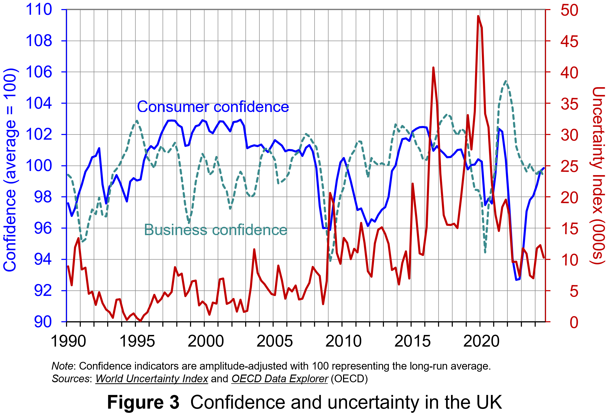 Figure 3 suggests that the relationship between confidence and uncertainty is rather more complex than perhaps is generally understood (click here for a PowerPoint). Haddow, Hare, Hooley and Shakir (see link below) argue that the evidence tends to point to changes in uncertainty affecting confidence, but with less evidence that changes in confidence affect uncertainty.
To illustrate this, consider the global financial crisis of the late 2000s. The argument can be made that the heightened uncertainty about future prospects for households and businesses helped to erode their confidence in the future. The result was that people and businesses revised down their expectations of the future (pessimism). However, although people were more pessimistic about the future, this was more likely to have been the result of uncertainty rather than the cause of further uncertainty.
Conclusion
For economists and policymakers alike, indicators of uncertainty, such as the Ahir, Bloom and Furceri World Uncertainty Index, are invaluable tools in understanding and forecasting behaviour and the likely economic outcomes that follow. Some uncertainty is inevitable, but the persistence of greater uncertainty since the global financial crisis of the late 2000s compares quite starkly with the relatively lower and more stable levels of uncertainty seen from the mid-1990s up to the crisis. Hence the recent frequency and size of changes in uncertainty show how important it to understand how uncertainty effects transmit through economies.
Academic papers
- The World Uncertainty Index
National Bureau of Economic Research, Working Paper 29763, Hites Ahir, Nicholas Bloom and Davide Furceri (February 2022)
- The Buffer-Stock Theory of Saving: Some Macroeconomic Evidence
Brookings Papers on Economic Activity, Christopher D Carroll (Vol 2, 1992)
- Macroeconomic uncertainty: what is it, how can we measure it and why does it matter?
Bank of England Quarterly Bulletin, 2013 Q2, Abigail Haddow, Chris Hare, John Hooley and Tamarah Shakir (13/6/13)
Articles
Data
Questions
- (a) Explain what is meant by the concept of diminishing marginal utility of consumption.
(b) Explain how this concept helps us to understand both consumption smoothing and the motivation to engage in buffer-stock saving.
- Explain the distinction between confidence and uncertainty when analysing macroeconomic shocks.
- Discuss which types of expenditures you think are likely to be most susceptible to uncertainty shocks.
- Discuss how economic uncertainty might affect productivity and the growth of potential output.
- How might the interconnectedness of economies affect the transmission of uncertainty effects through economies?
 A common practice of international investors is to take part in the so-called ‘carry trade’. This involves taking advantage of nominal interest rate differences between countries. For example, assume that interest rates are low in Japan and high in the USA. It is thus profitable to borrow yen in Japan at the low interest rate, exchange it into US dollars and deposit the money at the higher interest rate available in the USA. If there is no change in the exchange rate between the dollar and the yen, the investor makes a profit equal to the difference in the interest rates.
Rather than depositing the money in a US bank account, an alternative is to purchase US bonds or other assets in the USA, where the return is again higher than that in Japan.
If, however, interest-rate differentials narrow, there is the possibility of the carry trade ‘unwinding’. Not only may the carry trade prove unprofitable (or less so), but investors may withdraw their deposits and pay back the loans. This, as we shall, can have adverse consequences on exchange rates.
The problem of an unwinding of the carry trade is not new. It worsened the underlying problems of the financial crisis in 2008. The question today is whether history is about to repeat itself with a new round of unwinding of the carry trade threatening economic growth and recovery around the world.
We start by looking at what happened in 2008.
The carry trade and the 2008 financial crisis
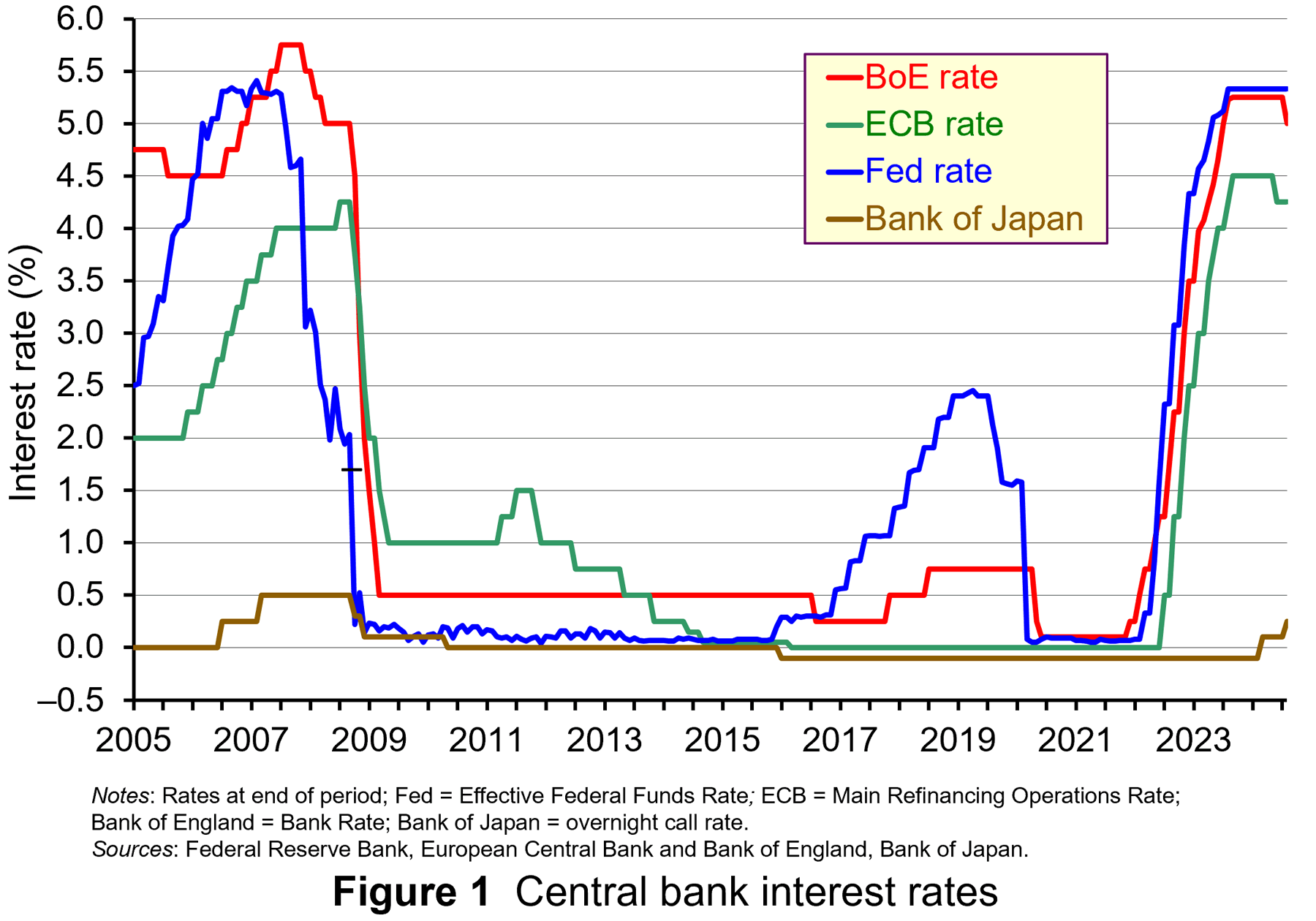 Prior to the financial crisis of 2008, current account deficit countries, such as the UK, USA and Australia, typically had relatively high interest rates, while current account surplus countries such as Japan and Switzerland had relatively low ones. Figure 1 shows central bank interest rates from 2005 to the current day (click here for a PowerPoint).
The carry trade saw investors borrowing money in Japan and Switzerland, exchanging it on the foreign exchange market, with the currency then deposited in the UK, USA and Australia. Hundreds of billions worth of dollars were involved in this carry trade.
If, however, the higher interest rates in the UK and other deficit countries were simply to compensate investors for the risk of currency depreciation, then there would be no excessive inflow of finance. The benefit of the higher interest rate would be offset by a depreciating currency. But the carry trade had the effect of making deficit currencies appreciate, thereby further boosting the carry trade by speculation of further exchange rate rises.
Thus the currencies of deficit countries appreciated, making their goods less competitive and worsening their current account deficit. Between 1996 and 2006, the average current account deficits as a percentage of GDP for Australia, the USA and the UK were close to 4½, 4 and 2, respectively. Between January 1996 and December 2006, the broad-based real exchange rate index of the Australian dollar appreciated by 17%, of the US dollar by 4% and of sterling by some 23%.
 Currencies of surplus countries depreciated, making their goods more competitive and further boosting their current account surpluses. For example, between 2004 and 2006 the average current account surpluses as a percentage of GDP for Japan and Switzerland were 3½ and 13, respectively. Their short-term interest rates averaged a mere 0.1% and 1.0% respectively (compared with 3.4%, 4.7% and 5.7% for the USA, the UK and Australia). Yet between January 2004 and December 2006, the real exchange rate index of the yen depreciated by 21%, while that of the Swiss franc depreciated by 6%.
With the credit crunch of 2007/8, the carry trade unwound. Much of the money deposited in the USA had been in highly risky assets, such as sub-prime mortgages. Investors scrambled to sell their assets in the USA, UK and the EU. Loans from Japan and Switzerland were repaid and these countries, seen as ‘safe havens’, attracted deposits. The currencies of deficit countries, such as the UK and USA, began to depreciate and those of surplus countries, such as Japan and Switzerland, began to appreciate. Between September 2007 and September 2008, the real exchange rate indices of the US dollar and sterling depreciated by 2% and 13% respectively; the yen and the Swiss franc appreciated by 3% and 2¾%.
This represented a ‘double whammy’ for Japanese exporters. Not only did its currency appreciate, making its exports more expensive in dollars, euros, pounds, etc., but the global recession saw consumers around the world buying less. As a result, the Japanese economy suffered the worst recession of the G7 economies.
The carry trade in recent months
Since 2016, there has been a re-emergence of the carry trade as the Fed began raising interest rates while the Bank of Japan kept rates at the ultra low level of –0.1% (see Figure 1). The process slowed down when the USA lowered interest rates in 2020 in response to the pandemic and fears of recession. But when the USA, the EU and the UK began raising rates at the beginning of 2022 in response to global inflationary pressures, while Japan kept its main rate at –0.1%, so the carry trade resumed in earnest. Cross-border loans originating in Japan (not all of it from the carry trade) had risen to ¥157tn ($1tn) by March 2024 – a rise of 21% from 2021.
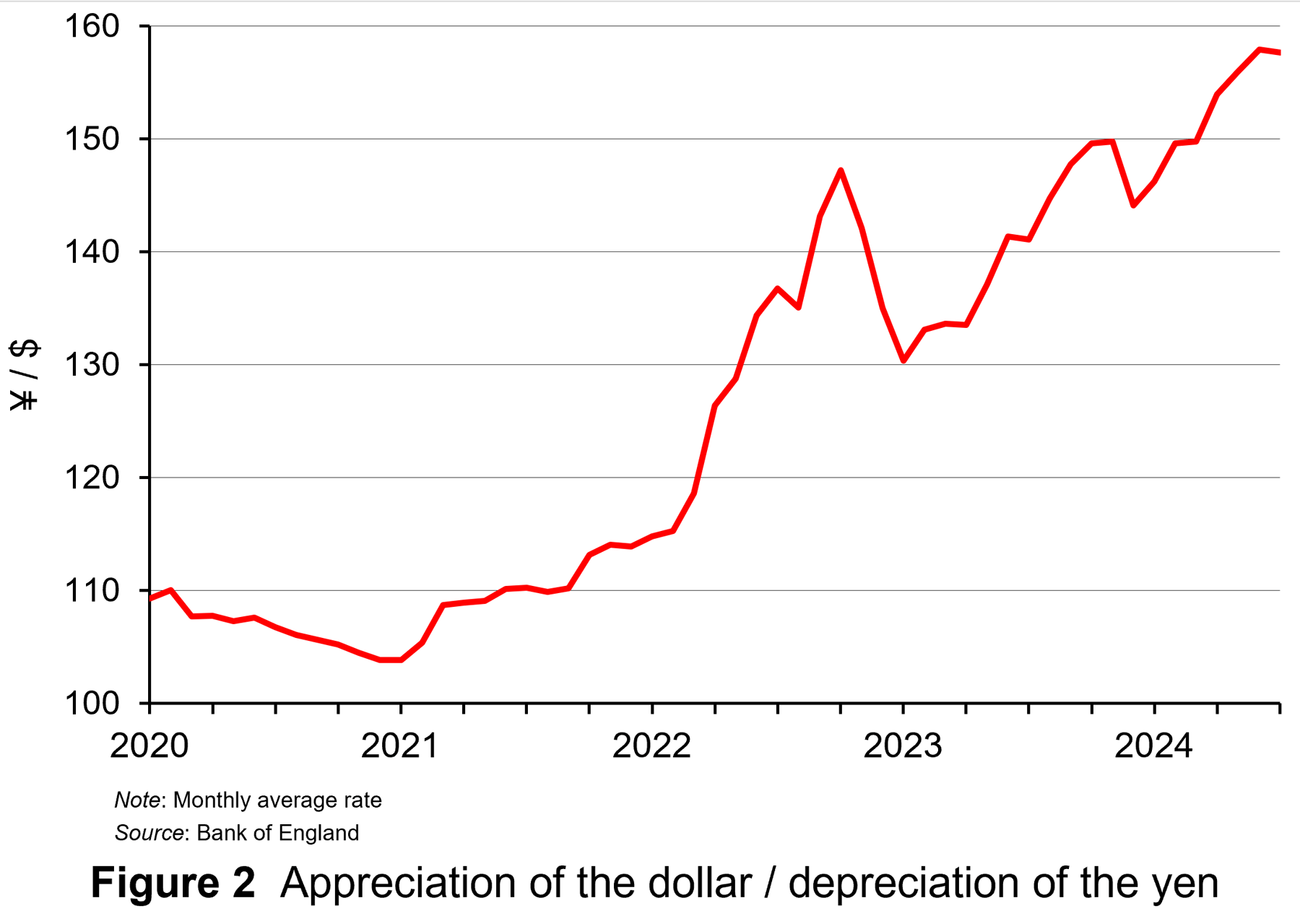 The process boosted US stock markets and contributed to the dollar appreciating against the yen (see Figure 2: click here for a PowerPoint).
Although this depreciation of the yen helped Japanese exports, it also led to rising prices. Japanese inflation rose steadily throughout 2022. In the 12 months to January 2022 the inflation rate was 0.5% (having been negative from October 2020 to August 2021). By January 2023, the annual rate had risen to 4.3% – a rate not seen since 1981. The Bank of Japan was cautious about raising interest rates to suppress this inflation, however, for fear of damaging growth and causing the exchange rate to appreciate and thereby damaging exports. Indeed, quarterly economic growth fell from 1.3% in 2023 Q1 to –1.0% in 2023 Q3.
But then, with growth rebounding and the yen depreciating further, in March 2024 the Bank of Japan decided to raise its key rate from –0.1% to 0.1%. This initially had the effect of stabilising the exchange rate. But then with the yen depreciating further and inflation rising from 2.5% to 2.8% in May and staying at this level in June, the Bank of Japan increased the key rate again at the end of July – this time to 0.25% – and there were expectations that there would be another rise before the end of the year.
At the same time, there were expectations that the Fed would soon lower its main rate (the Federal Funds Rate) from its level of 5.33%. The ECB and the Bank of England had already begun lowering their main rates in response to lower inflation. The carry trade rapidly unwound. Investors sold US, EU and UK assets and began repaying yen loans.
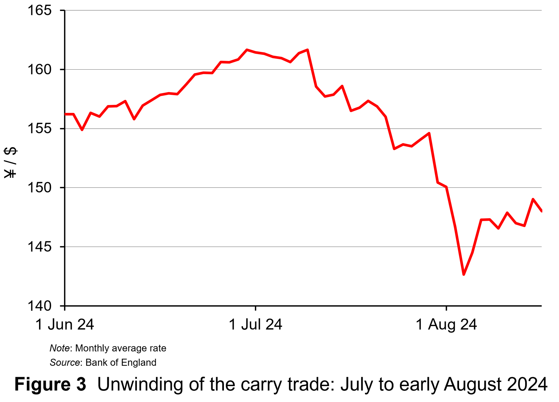 The result was a rapid appreciation of the yen as Figure 3 shows (click here for a PowerPoint). Between 31 July (the date the Bank of Japan raised interest rates the second time) and 5 August, the dollar depreciated against the yen from ¥150.4 to ¥142.7. In other words, the value of 100 yen appreciated from $0.66 to $0.70 – an appreciation of the yen of 6.1%.
Fears about the unwinding of the carry trade led to falls in stock markets around the world. Not only were investors selling shares to pay back the loans, but fears of the continuing process put further downward pressure on shares. From 31 July to 5 August, the US S&P 500 fell by 6.1% and the tech-heavy Nasdaq by 8.0%.
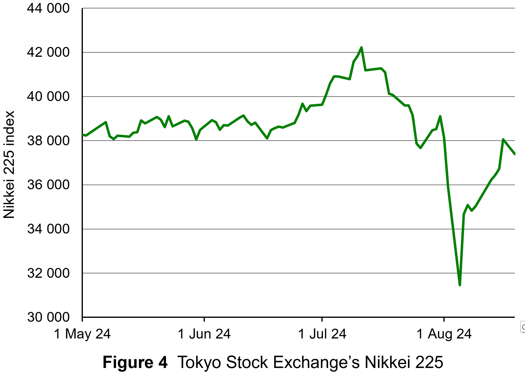 As far as the Tokyo stock market was concerned, the appreciation of the yen sparked fears that the large Japanese export sector would be damaged. Investors rushed to sell shares. Between 31 July and 5 August, the Nikkei 225 (the main Japanese stock market index) fell by 19.5% – its biggest short-term fall ever (see Figure 4: click here for a PowerPoint).
Although the yen has since depreciated slightly (a rise in the yen/dollar rate) and stock markets have recovered somewhat, expectations of many investors are that the unwinding of the yen carry trade has some way to go. This could result in a further appreciation of the yen from current levels of around ¥100 = $0.67 to around $0.86 in a couple of years’ time.
There are also fears about the carry trade in the Chinese currency, the yuan. Some $500 billion of foreign currency holdings have been acquired with yuan since 2022. As with the Japanese carry trade, this has been encouraged by low Chinese interest rates and a depreciating yuan. Not only are Chinese companies investing abroad, but foreign companies operating in China have been using their yuan earnings from their Chinese operations to invest abroad rather than in China. The Chinese carry trade, however, has been restricted by the limited convertibility of the yuan. If the Chinese carry trade begins to unwind when the Chinese economy begins to recover and interest rates begin to rise, the effect will probably be more limited than with the yen.
Articles
- A popular trading strategy just blew up in investors’ faces
CNN, Allison Morrow (7/8/24)
- The big ‘carry trade’ unwind is far from over, strategists warn
CNBC, Sam Meredith (13/8/24)
- Unwinding of yen ‘carry trade’ still threatens markets, say analysts
Financial Times, Leo Lewis and David Keohane (7/8/24)
- The yen carry trade sell-off marks a step change in the business cycle
Financial Times, John Plender (10/8/24)
- Forbes Money Markets Global Markets React To The Japanese Yen Carry Trade Unwind
Forbes, Frank Holmes (12/8/24)
- 7 unwinding carry trades that crashed the markets
Alt21 (26/1/23)
- A carry crash also kicked off the global financial crisis 17 years ago — here’s why it’s unlikely to get as bad this time
The Conversation, Charles Read (9/8/24)
- What is the Chinese yuan carry trade and how is it different from the yen’s?
Reuters, Winni Zhou and Summer Zhen (13/8/24)
- Carry Trade That Blew Up Markets Is Attracting Hedge Funds Again
Yahoo Finance/Bloomberg, David Finnerty and Ruth Carson (16/8/24)
- Currency Carry Trades 101
Investopedia, Kathy Lien (9/8/24)
- Carry Trades Torpedoed The Market. They’re Still Everywhere.
Finimize, Stéphane Renevier (13/8/24)
Questions
- What factors drive the currency carry trade?
- Is the carry trade a form of arbitrage?
- Find out and explain what has happened to the Japanese yen since this blog was written.
- Find out and explain some other examples of carry trades.
- Why are expectations so important in determining the extent and timing of the unwinding of carry trades?
 The past decade or so has seen large-scale economic turbulence. As we saw in the blog Fiscal impulses, governments have responded with large fiscal interventions. The COVID-19 pandemic, for example, led to a positive fiscal impulse in the UK in 2020, as measured by the change in the structural primary balance, of over 12 per cent of national income.
The scale of these interventions has led to a significant increase in the public-sector debt-to-GDP ratio in many countries. The recent interest rates hikes arising from central banks responding to inflationary pressures have put additional pressure on the financial well-being of governments, not least on the financing of their debt. Here we discuss these pressures in the context of the ‘r – g’ rule of sustainable public debt.
Public-sector debt and borrowing
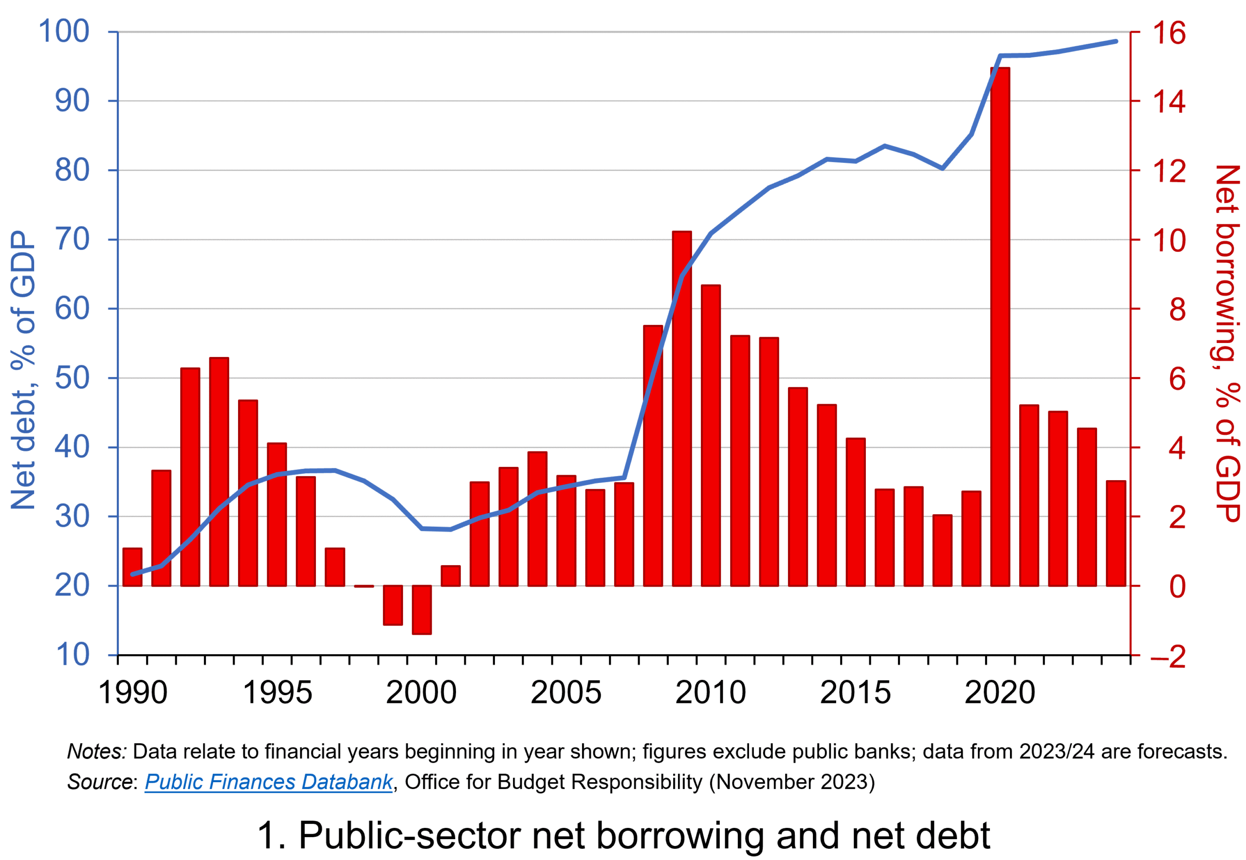 Chart 1 shows the path of UK public-sector net debt and net borrowing, as percentages of GDP, since 1990. Debt is a stock concept and is the result of accumulated flows of past borrowing. Net debt is simply gross debt less liquid financial assets, which mainly consist of foreign exchange reserves and cash deposits. Net borrowing is the headline measure of the sector’s deficit and is based on when expenditures and receipts (largely taxation) are recorded rather than when cash is actually paid or received. (Click here for a PowerPoint of Chart 1)
Chart 1 shows the impact of the fiscal interventions associated with the global financial crisis and the COVID-19 pandemic, when net borrowing rose to 10 per cent and 15 per cent of GDP respectively. The former contributed to the debt-to-GDP ratio rising from 35.6 per cent in 2007/8 to 81.6 per cent in 2014/15, while the pandemic and subsequent cost-of-living interventions contributed to the ratio rising from 85.2 per cent in 2019/20 to around 98 per cent in 2023/24.
Sustainability of the public finances
 The ratcheting up of debt levels affects debt servicing costs and hence the budgetary position of government. Yet the recent increases in interest rates also raise the costs faced by governments in financing future deficits or refinancing existing debts that are due to mature. In addition, a continuation of the low economic growth that has beset the UK economy since the global financial crisis also has implications for the burden imposed on the public sector by its debts, and hence the sustainability of the public finances. After all, low growth has implications for spending commitments, and, of course, the flow of receipts.
The analysis therefore implies that the sustainability of public-sector debt is dependent on at least three factors: existing debt levels, the implied average interest rate facing the public sector on its debts, and the rate of economic growth. These three factors turn out to underpin a well-known rule relating to the fiscal arithmetic of public-sector debt. The rule is sometimes known as the ‘r – g’ rule (i.e. the interest rate minus the growth rate).
Underpinning the fiscal arithmetic that determines the path of public-sector debt is the concept of the ‘primary balance’. This is the difference between the sector’s receipts and its expenditures less its debt interest payments. A primary surplus (a positive primary balance) means that receipts exceed expenditures less debt interest payments, whereas a primary deficit (a negative primary balance) means that receipts fall short. The fiscal arithmetic necessary to prevent the debt-to-GDP ratio rising produces the following stable debt equation or ‘r – g’ rule:
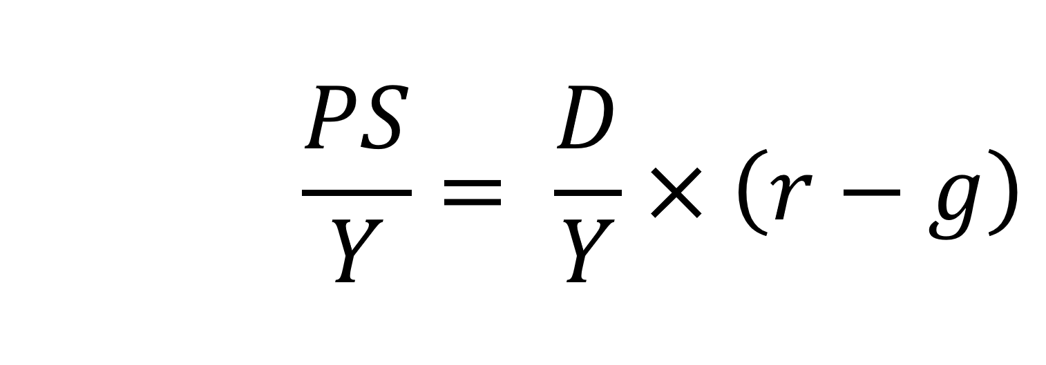
On the left-hand side of the stable debt equation is the required primary surplus (PS) to GDP (Y) ratio. Moving to the right-hand side, the first term is the existing debt-to-GDP ratio (D/Y). The second term ‘r – g’, is the differential between the average implied interest rate the government pays on its debt and the growth rate of the economy. These terms can be expressed in either nominal or real terms as this does not affect the differential.
To illustrate the rule consider a country whose existing debt-to-GDP ratio is 1 (i.e. 100 per cent) and the ‘r – g’ differential is 0.02 (2 percentage points). In this scenario they would need to run a primary surplus to GDP ratio of 0.02 (i.e. 2 percent of GDP).
The ‘r – g‘ differential
The ‘r – g’ differential reflects macroeconomic and financial conditions. The fiscal arithmetic shows that these are important for the dynamics of public-sector debt. The fiscal arithmetic is straightforward when r = g as any primary deficit will cause the debt-to-GDP ratio to rise, while a primary surplus will cause the ratio to fall. The larger is g relative to r the more favourable are the conditions for the path of debt. Importantly, if the differential is negative (r < g), it is possible for the public sector to run a primary deficit, up to the amount that the stable debt equation permits.
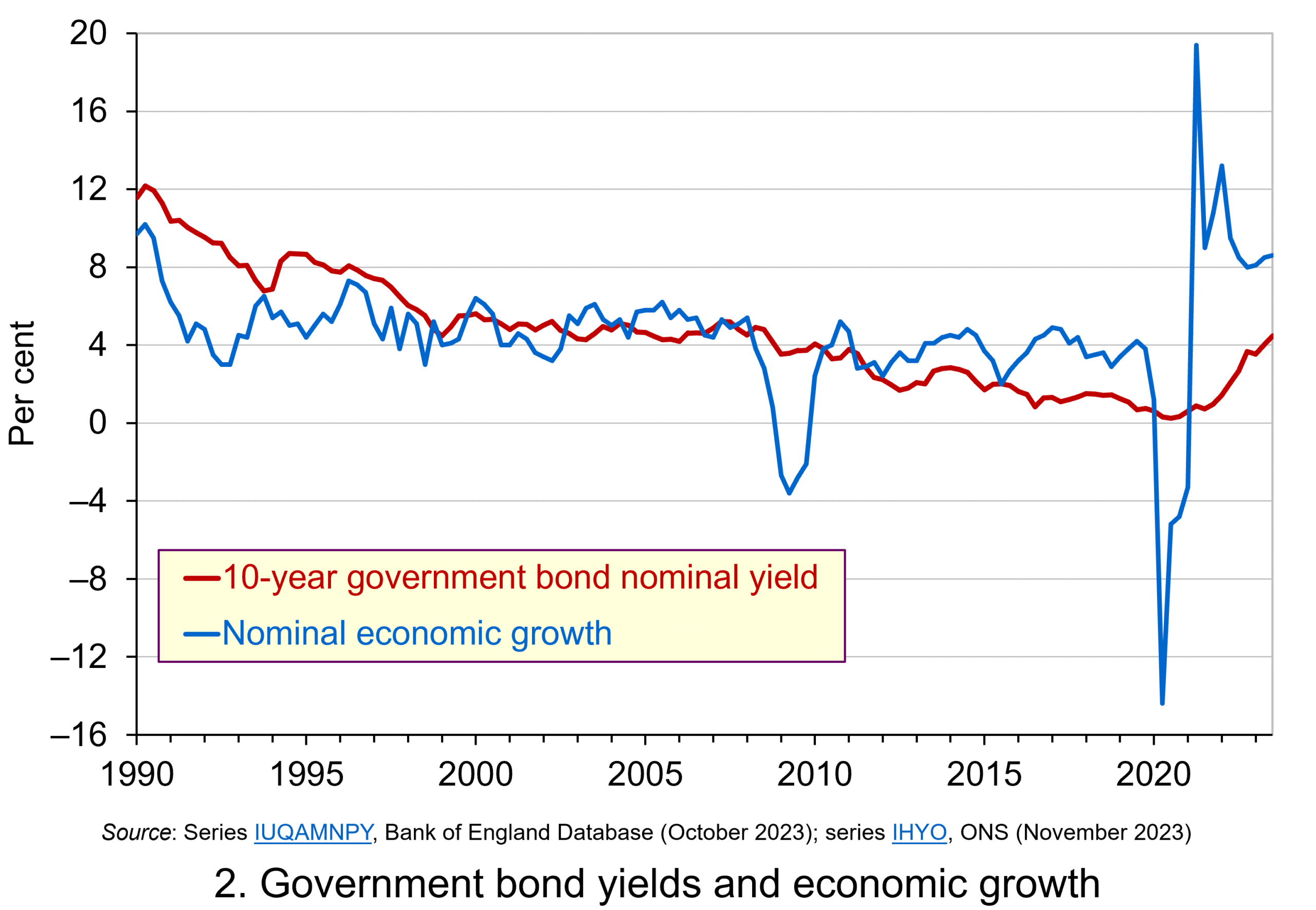 Consider Charts 2 and 3 to understand how the ‘r – g’ differential has affected debt sustainability in the UK since 1990. Chart 2 plots the implied yield on 10-year government bonds, alongside the annual rate of nominal growth (click here for a PowerPoint). As John explains in his blog The bond roller coaster, the yield is calculated as the coupon rate that would have to be paid for the market price of a bond to equal its face value. Over the period, the average annual nominal growth rate was 4.5 per cent, while the implied interest rate was almost identical at 4.6 per cent. The average annual rate of CPI inflation over this period was 2.8 per cent.
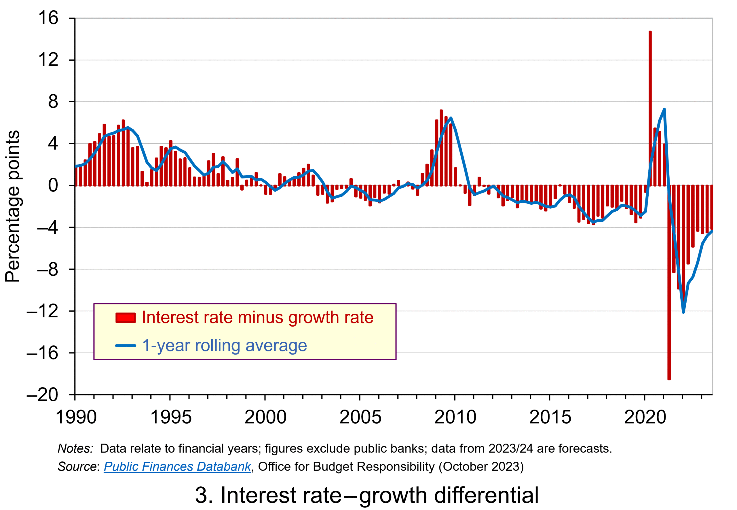 Chart 3 plots the ‘r – g’ differential which is simply the difference between the two series in Chart 2, along with a 12-month rolling average of the differential to help show better the direction of the differential by smoothing out some of the short-term volatility (click here for a PowerPoint). The differential across the period is a mere 0.1 percentage points implying that macroeconomic and financial conditions have typically been neutral in supporting debt sustainability. However, this does mask some significant changes across the period.
We observe a general downward trend in the ‘r – g’ differential from 1990 up to the time of the global financial crisis. Indeed between 2003 and 2007 we observe a favourable negative differential which helps to support the sustainability of public debt and therefore the well-being of the public finances. This downward trend of the ‘r – g’ differential was interrupted by the financial crisis, driven by a significant contraction in economic activity. This led to a positive spike in the differential of over 7 percentage points.
 Yet the negative differential resumed in 2010 and continued up to the pandemic. Again, this is indicative of the macroeconomic and financial environments being supportive of the public finances. It was, however, largely driven by low interest rates rather than by economic growth.
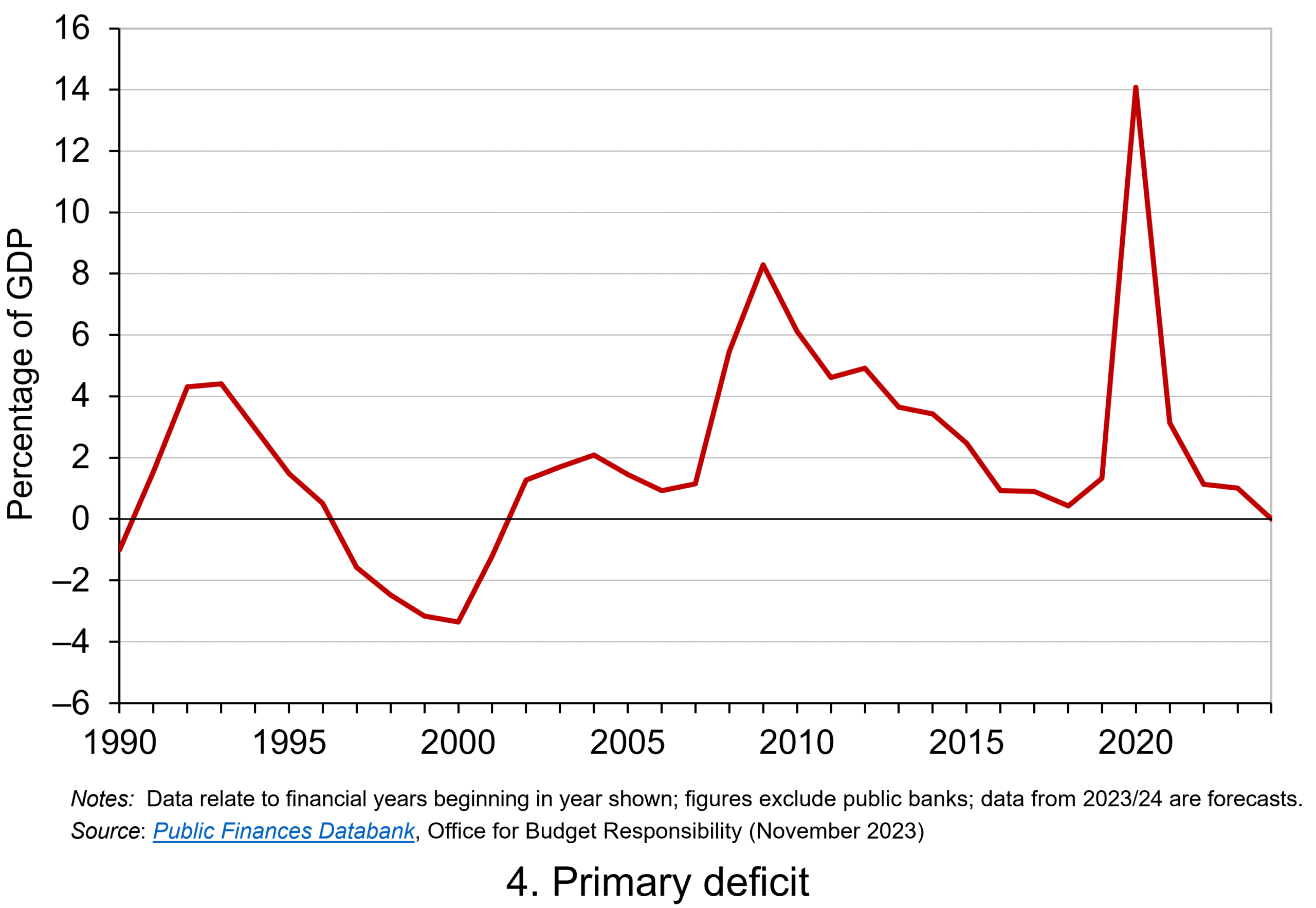
Consequently, the negative ‘r – g’ differential meant that the public sector could continue to run primary deficits during the 2010s, despite the now much higher debt-to-GDP ratio. Yet, weak growth was placing limits on this. Chart 4 indeed shows that primary deficits fell across the decade (click here for a PowerPoint).
The pandemic and beyond
 The pandemic saw the ‘r – g’ differential again turn markedly positive, averaging 7 percentage points in the four quarters from Q2 of 2020. While the differential again turned negative, the debt-to-GDP ratio had also increased substantially because of large-scale fiscal interventions. This made the negative differential even more important for the sustainability of the public finances. The question is how long the negative differential can last.
Looking forward, the fiscal arithmetic is indeed uncertain and worryingly is likely to be less favourable. Interest rates have risen and, although inflationary pressures may be easing somewhat, interest rates are likely to remain much higher than during the past decade. Geopolitical tensions and global fragmentation pose future inflationary concerns and a further drag on growth.
As well as the short-term concerns over growth, there remain long-standing issues of low productivity which must be tackled if the growth of the UK economy’s potential output is to be raised. These concerns all point to the important ‘r – g’ differential become increasingly less negative, if not positive. If so the fiscal arithmetic could mean increasingly hard maths for policymakers.
Articles
- The budget deficit: a short guide
House of Commons Library (8/6/23)
- If markets are right about long real rates, public debt ratios will increase for some time. We must make sure that they do not explode.
Peterson Institute for International Economics, Olivier Blanchard (6/11/23)
- The UK government’s debt nightmare
ITV News, Robert Peston (13/7/23)
- National debt could hit 300% of GDP by 2070s, independent watchdog the OBR warns
Sky News, James Sillars (13/7/23)
- How much money is the UK government borrowing, and does it matter?
BBC News (20/10/23)
- Cost of national debt hits 20-year high
BBC News, Vishala Sri-Pathma & Faisal Islam (4/10/23)
- Bond markets could see ‘mini boom-bust cycles’ as global government debt to soar by $5 trillion a yea
Markets Insider, Filip De Mott (16/11/23)
- The counterintuitive truth about deficits for bond investors
Financial Times, Matt King (17/11/23)
- UK government borrowing almost £20bn lower than expected
The Guardian, Richard Partington (20/10/23)
- Controlling debt is just a means — it is not a government’s end
Financial Times, Martin Wolf (13/11/23)
Data
Questions
- What is meant by each of the following terms: (a) net borrowing; (b) primary deficit; (c) net debt?
- Explain how the following affect the path of the public-sector debt-to-GDP ratio: (a) interest rates; (b) economic growth; (c) the existing debt-to-GDP ratio.
- Which factors during the 2010s were affecting the fiscal arithmetic of public debt positively, and which negatively?
- Discuss the prospects for the fiscal arithmetic of public debt in the coming years.
- Assume that a country has an existing public-sector debt-to-GDP ratio of 60 percent.
(a) Using the ‘rule of thumb’ for public debt dynamics, calculate the approximate primary balance it would need to run in the coming year if the expected average real interest rate on the debt were 3 per cent and real economic growth were 2 per cent?
(b) Repeat (a) but now assume that real economic growth is expected to be 4 per cent.
(c) Repeat (a) but now assume that the existing public-sector debt-to-GDP ratio is 120 per cent.
(d) Using your results from (a) to (c) discuss the factors that affect the fiscal arithmetic of the growth of public-sector debt.
 Those of a certain age may remember the fanfare which heralded the introduction of the Single European market (SEM) on 1 January 1993. It promised the removal of internal barriers to the movement of goods, services, capital and people. One sector that was noticeably absent from the single market, however, was banking.
 Even as the EU moved towards economic and monetary union (EMU) during the 1990s, there was no discussion of integration for the banking industry. However, that changed following the 2008 financial crisis and 2011 eurozone crisis. Both episodes exposed vulnerabilities in the EU banking system which required taxpayer support. It was proposed that deeper integration of the banking sector would ensure its stability and resilience. This stimulated moves towards European Banking Union (EBU), starting with the European Council agreeing its creation in 2012. There are three institutional pillars to the Union:
 1. Ring fencing. Although there is a single supervisory mechanism for large systemically important institutions, since the financial crisis national regulators have implemented ‘ring-fencing’. This aims to protect retail banking activities from riskier investment banking. Ring-fencing retains liquidity, dividends and other bank assets within national borders to protect their retail banking sectors from contagion. The ECB estimates €225 billion of capital and €250 billion of liquidity is trapped by such national restrictions. Further, unharmonized and unpredictable use of capital buffers adds complexity for capital management at a multinational level. This particularly impacts large institutions. Banks’ cross-border activities are impeded since they are restricted in the way they can use capital and liquidity across the bloc.
 On the demand-side, retail banking is largely a relational rather than a transactional service, with consumption taking place over a long time-period with significant financial risks attached. Even with deposit insurance and a lender of last resort (the central bank), consumers exhibit significant loss aversion in their use of retail banking services. Consequently, trust and confidence are important characteristics for consumers and that means they are likely to prefer to use familiar domestic institutions.
  Some argue that retail banking is a public utility and should be regulated as such. It has a simple business model, taking deposits, making payments and making loans. Like other utilities, such as water and energy, retail banking is an essential service for the smooth functioning of the economy and society. Like other utilities, bank failures create severe problems for the economy and society.
  The UK’s poor record on productivity since the 2008 financial crisis is well documented, not least in this blog series. Output per worker has flatlined over the 17 years since the crisis. As was noted in the blog,
  From Figure 1 it can be observed that, since the mid-1990s, the UK has consistently had lower investment as a percentage of GDP compared to other significant developed market economies. The cumulative effect of this gap has contributed to lower productivity and lower economic growth.
 Analysis by the OECD suggest that, while the cost of financing investment has declined since the financial crisis, the gap between this and the hurdle rate used to appraise investments has widened. Between 2010 and 2021 the difference nearly doubled to 4%. This increase in the hurdle rate can be related to increases in the expected rate of return by UK companies and their investors.
 However, it is not interest rates that have increased the opportunity cost, and hence the minimum expected rate of return associated with investment, in the UK since the financial crisis. For most of the period since 2008, interest rates have been extremely low, sitting at below 1%, only rising significantly during the post-pandemic inflationary surge in 2022. This indicates that this source of opportunity cost for the commitment of business investment has been extremely low.
 There has been much discussion of increased uncertainty and risk aversion among global investors and firms (see the blogs
  Figure 2 illustrates the monthly index from 1998 to July 2025. The series is normalised to standard deviation 1 prior to 2011 and then summed across papers, by month. Then, the series is normalised to mean 100 prior to 2011.
 Over the past 10 years, policy uncertainty has played a significant role in deterring investment. So, if there is greater continuity, this may then promote higher levels of investment.
 Figure 1 (click
  As Figure 2 shows (click
  The theory of buffer-stock saving was popularised by Christopher Carroll in 1992 (see link below). It implies that in the presence of uncertainty, people are prepared to consume less today in order to increase levels of saving, pay off existing debts, or borrow less relative to that in the absence of uncertainty. The extent of the buffer of financial wealth that people want to hold will depend on their own appetite for risk, the level of uncertainty, and the moderating effect from their own impatience and, hence, present bias for consuming today.
 Figure 3 suggests that the relationship between confidence and uncertainty is rather more complex than perhaps is generally understood (click
  A common practice of international investors is to take part in the so-called ‘carry trade’. This involves taking advantage of nominal interest rate differences between countries. For example, assume that interest rates are low in Japan and high in the USA. It is thus profitable to borrow yen in Japan at the low interest rate, exchange it into US dollars and deposit the money at the higher interest rate available in the USA. If there is no change in the exchange rate between the dollar and the yen, the investor makes a profit equal to the difference in the interest rates.
 Prior to the financial crisis of 2008, current account deficit countries, such as the UK, USA and Australia, typically had relatively high interest rates, while current account surplus countries such as Japan and Switzerland had relatively low ones. Figure 1 shows central bank interest rates from 2005 to the current day (click
  Currencies of surplus countries depreciated, making their goods more competitive and further boosting their current account surpluses. For example, between 2004 and 2006 the average current account surpluses as a percentage of GDP for Japan and Switzerland were 3½ and 13, respectively. Their short-term interest rates averaged a mere 0.1% and 1.0% respectively (compared with 3.4%, 4.7% and 5.7% for the USA, the UK and Australia). Yet between January 2004 and December 2006, the real exchange rate index of the yen depreciated by 21%, while that of the Swiss franc depreciated by 6%.
 The process boosted US stock markets and contributed to the dollar appreciating against the yen (see Figure 2: click
  The result was a rapid appreciation of the yen as Figure 3 shows (click
  As far as the Tokyo stock market was concerned, the appreciation of the yen sparked fears that the large Japanese export sector would be damaged. Investors rushed to sell shares. Between 31 July and 5 August, the Nikkei 225 (the main Japanese stock market index) fell by 19.5% – its biggest short-term fall ever (see Figure 4: click
  The past decade or so has seen large-scale economic turbulence. As we saw in the blog
  Chart 1 shows the path of UK public-sector net debt and net borrowing, as percentages of GDP, since 1990. Debt is a stock concept and is the result of accumulated flows of past borrowing. Net debt is simply gross debt less liquid financial assets, which mainly consist of foreign exchange reserves and cash deposits. Net borrowing is the headline measure of the sector’s deficit and is based on when expenditures and receipts (largely taxation) are recorded rather than when cash is actually paid or received. (Click
  The ratcheting up of debt levels affects debt servicing costs and hence the budgetary position of government. Yet the recent increases in interest rates also raise the costs faced by governments in financing future deficits or refinancing existing debts that are due to mature. In addition, a continuation of the low economic growth that has beset the UK economy since the global financial crisis also has implications for the burden imposed on the public sector by its debts, and hence the sustainability of the public finances. After all, low growth has implications for spending commitments, and, of course, the flow of receipts.
 Consider Charts 2 and 3 to understand how the ‘r – g’ differential has affected debt sustainability in the UK since 1990. Chart 2 plots the implied yield on 10-year government bonds, alongside the annual rate of nominal growth (click
  Chart 3 plots the ‘r – g’ differential which is simply the difference between the two series in Chart 2, along with a 12-month rolling average of the differential to help show better the direction of the differential by smoothing out some of the short-term volatility (click
  Yet the negative differential resumed in 2010 and continued up to the pandemic. Again, this is indicative of the macroeconomic and financial environments being supportive of the public finances. It was, however, largely driven by low interest rates rather than by economic growth.
  The pandemic saw the ‘r – g’ differential again turn markedly positive, averaging 7 percentage points in the four quarters from Q2 of 2020. While the differential again turned negative, the debt-to-GDP ratio had also increased substantially because of large-scale fiscal interventions. This made the negative differential even more important for the sustainability of the public finances. The question is how long the negative differential can last.