 We continue to live through incredibly turbulent times. In the past decade or so we have experienced a global financial crisis, a global health emergency, seen the UK’s departure from the European Union, and witnessed increasing levels of geopolitical tension and conflict. Add to this the effects from the climate emergency and it easy to see why the issue of economic uncertainty is so important when thinking about a country’s economic prospects.
In this blog we consider how we can capture this uncertainty through a World Uncertainty Index and the ways by which economic uncertainty impacts on the macroeconomic environment.
World Uncertainty Index
Hites Ahir, Nicholas Bloom and Davide Furceri have constructed a measure of uncertainty known as the World Uncertainty Index (WUI). This tracks uncertainty around the world using the process of ‘text mining’ the country reports produced by the Economist Intelligence Unit. The words searched for are ‘uncertain’, ‘uncertainty’ and ‘uncertainties’ and a tally is recorded based on the number of times they occur per 1000 words of text. To produce the index this figure is then multiplied up by 100 000. A higher number therefore indicates a greater level of uncertainty. For more information on the construction of the index see the 2022 article by Ahir, Bloom and Furceri linked below.
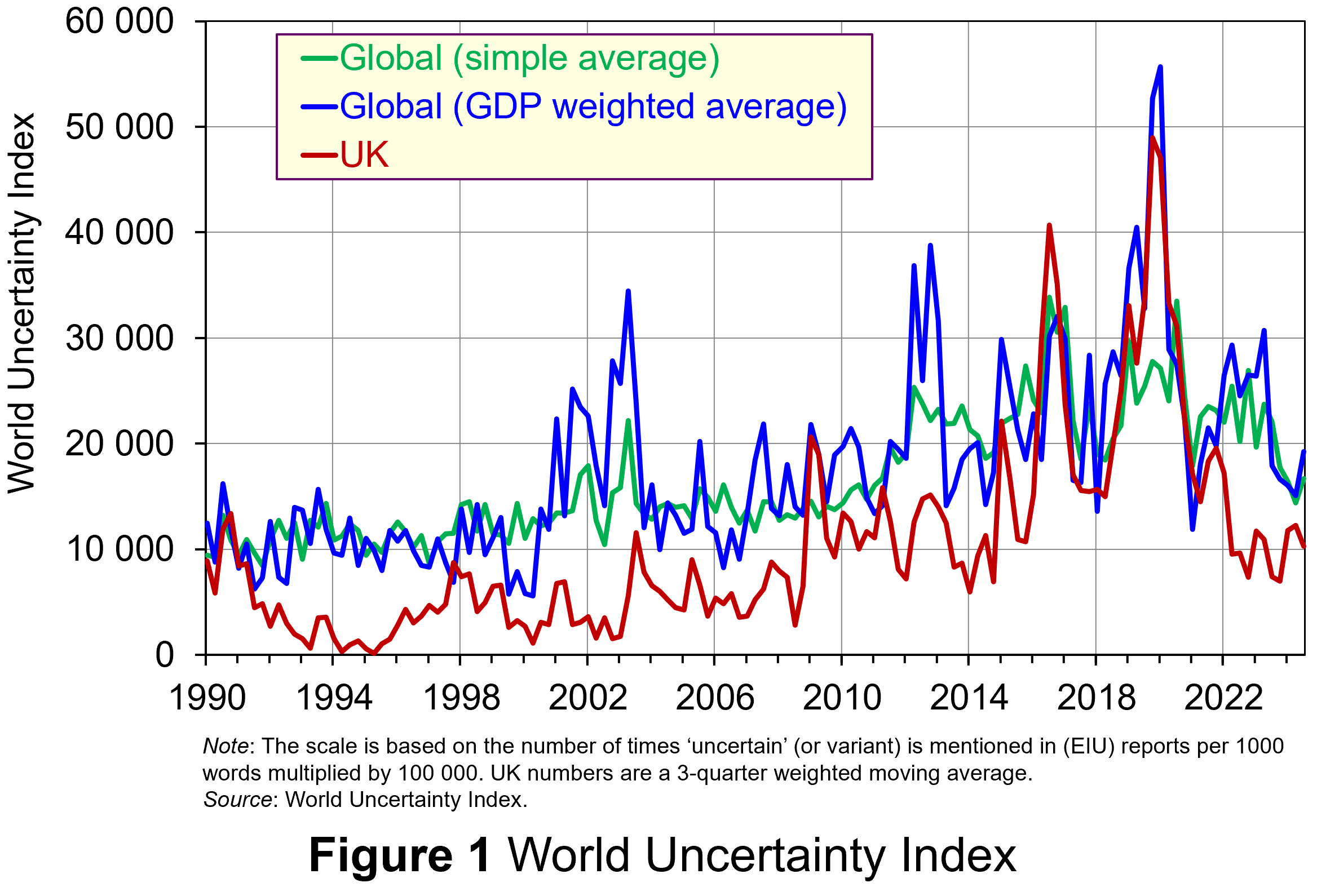 Figure 1 (click here for a PowerPoint) shows the WUI both globally and in the UK quarterly since 1991. The global index covers 143 countries and is presented as both a simple average and a GDP weighted average. The UK WUI is also shown. This is a three-quarter weighted average, the authors’ preferred measure for individual countries, where increasing weights of 0.1, 0.3 and 0.6 are used for the three most recent quarters.
From Figure 1 we can see how the level of uncertainty has been particularly volatile over the past decade or more. Events such as the sovereign debt crisis in parts of Europe in the early 2010s, the Brexit referendum in 2016, the COVID-pandemic in 2020–21 and the invasion of Ukraine in 2022 all played their part in affecting uncertainty domestically and internationally.
Uncertainty, risk-aversion and aggregate demand
Now the question turns to how uncertainty affects economies. One way of addressing this is to think about ways in which uncertainty affects the choices that people and businesses make. In doing so, we could think about the impact of uncertainty on components of aggregate demand, such as household consumption and investment, or capital expenditures by firms.
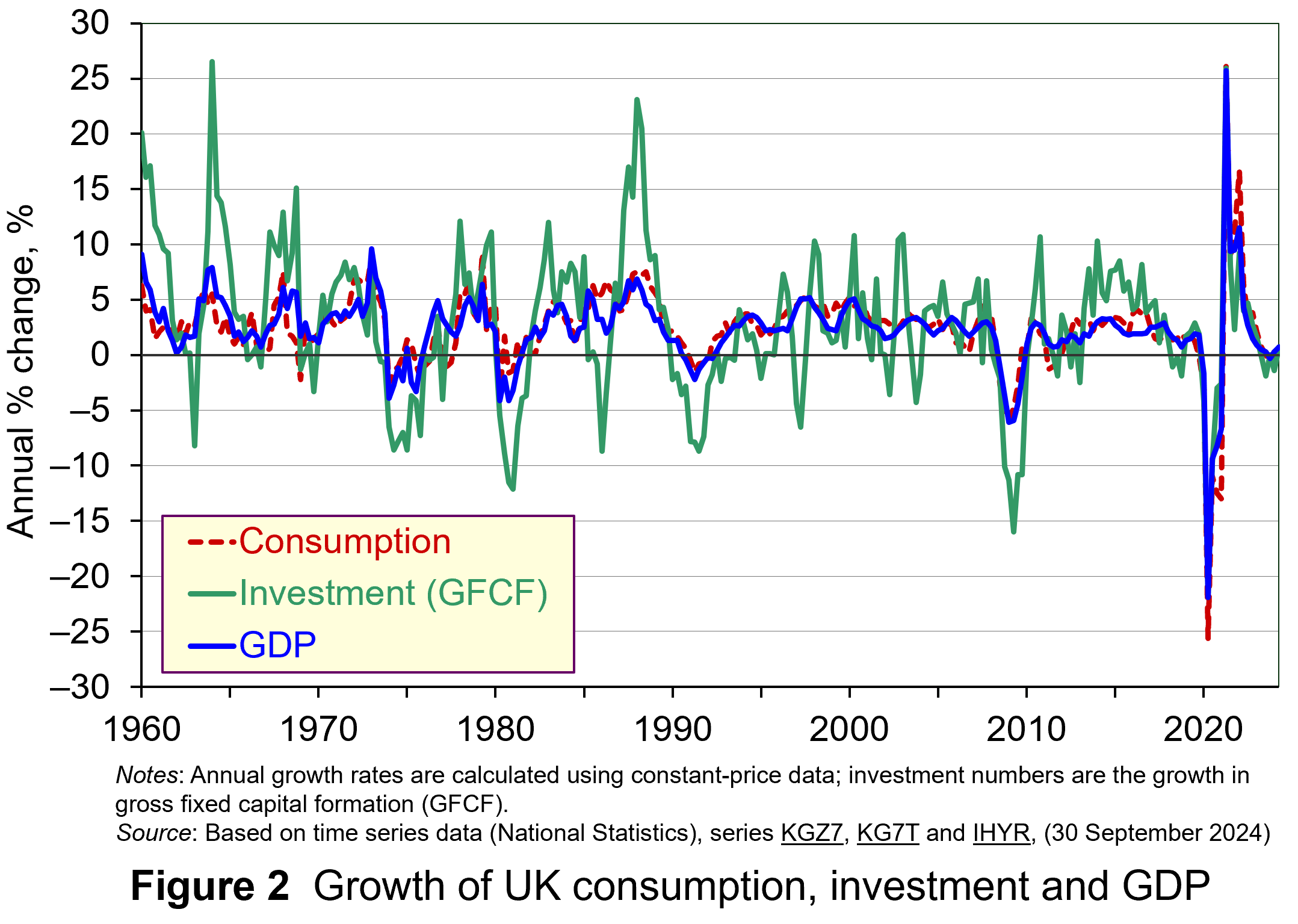 As Figure 2 shows (click here for a PowerPoint), investment is particularly volatile, and much more so than household spending. Some of this can be attributed to the ‘lumpiness’ of investment decisions since these expenditures tend to be characterised by indivisibility and irreversibility. This means that they are often relatively costly to finance and are ‘all or nothing’ decisions. In the context of uncertainty, it can make sense therefore for firms to wait for news that makes the future clearer. In this sense, we can think of uncertainty rather like a fog that firms are peering through. The thicker the fog, the more uncertain the future and the more cautious firms are likely to be.
The greater caution that many firms are likely to adopt in more uncertain times is consistent with the property of risk-aversion that we often attribute to a range of economic agents. When applied to household spending decisions, risk-aversion is often used to explain why households are willing to hold a buffer stock of savings to self-insure against unforeseen events and their future financial outcomes being worse than expected. Hence, in more uncertain times households are likely to want to increase this buffer further.
 The theory of buffer-stock saving was popularised by Christopher Carroll in 1992 (see link below). It implies that in the presence of uncertainty, people are prepared to consume less today in order to increase levels of saving, pay off existing debts, or borrow less relative to that in the absence of uncertainty. The extent of the buffer of financial wealth that people want to hold will depend on their own appetite for risk, the level of uncertainty, and the moderating effect from their own impatience and, hence, present bias for consuming today.
Risk aversion is consistent with the property of diminishing marginal utility of income or consumption. In other words, as people’s total spending volumes increase, their levels of utility or satisfaction increase but at an increasingly slower rate. It is this which explains why individuals are willing to engage with the financial system to reallocate their expected life-time earnings and have a smoother consumption profile than would otherwise be the case from their fluctuating incomes.
Yet diminishing marginal utility not only explains consumption smoothing, but also why people are willing to engage with the financial system to have financial buffers as self-insurance. It explains why people save more or borrow less today than suggested by our base-line consumption smoothing model. It is the result of people’s greater dislike (and loss of utility) from their financial affairs being worse than expected than their like (and additional utility) from them being better than expected. This tendency is only likely to increase the more uncertain times are. The result is that uncertainty tends to lower household consumption with perhaps ‘big-ticket items’, such as cars, furniture, and expensive electronic goods, being particularly sensitive to uncertainty.
Uncertainty and confidence
Uncertainty does not just affect risk; it also affects confidence. Risk and confidence are often considered together, not least because their effects in generating and transmitting shocks can be difficult to disentangle.
We can think of confidence as capturing our mood or sentiment, particularly with respect to future economic developments. Figure 3 plots the Uncertainty Index for the UK alongside the OECD’s composite consumer and business confidence indicators. Values above 100 for the confidence indicators indicate greater confidence about the future economic situation and near-term business environment, while values below 100 indicate pessimism towards the future economic and business environments.
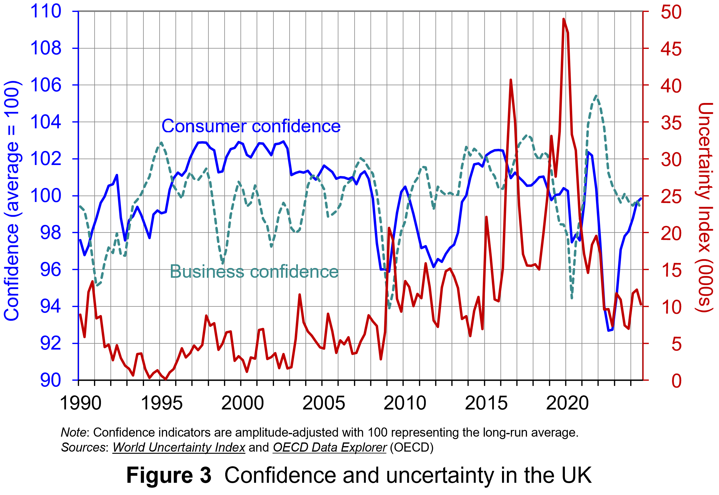 Figure 3 suggests that the relationship between confidence and uncertainty is rather more complex than perhaps is generally understood (click here for a PowerPoint). Haddow, Hare, Hooley and Shakir (see link below) argue that the evidence tends to point to changes in uncertainty affecting confidence, but with less evidence that changes in confidence affect uncertainty.
To illustrate this, consider the global financial crisis of the late 2000s. The argument can be made that the heightened uncertainty about future prospects for households and businesses helped to erode their confidence in the future. The result was that people and businesses revised down their expectations of the future (pessimism). However, although people were more pessimistic about the future, this was more likely to have been the result of uncertainty rather than the cause of further uncertainty.
Conclusion
For economists and policymakers alike, indicators of uncertainty, such as the Ahir, Bloom and Furceri World Uncertainty Index, are invaluable tools in understanding and forecasting behaviour and the likely economic outcomes that follow. Some uncertainty is inevitable, but the persistence of greater uncertainty since the global financial crisis of the late 2000s compares quite starkly with the relatively lower and more stable levels of uncertainty seen from the mid-1990s up to the crisis. Hence the recent frequency and size of changes in uncertainty show how important it to understand how uncertainty effects transmit through economies.
Academic papers
- The World Uncertainty Index
National Bureau of Economic Research, Working Paper 29763, Hites Ahir, Nicholas Bloom and Davide Furceri (February 2022)
- The Buffer-Stock Theory of Saving: Some Macroeconomic Evidence
Brookings Papers on Economic Activity, Christopher D Carroll (Vol 2, 1992)
- Macroeconomic uncertainty: what is it, how can we measure it and why does it matter?
Bank of England Quarterly Bulletin, 2013 Q2, Abigail Haddow, Chris Hare, John Hooley and Tamarah Shakir (13/6/13)
Articles
Data
Questions
- (a) Explain what is meant by the concept of diminishing marginal utility of consumption.
(b) Explain how this concept helps us to understand both consumption smoothing and the motivation to engage in buffer-stock saving.
- Explain the distinction between confidence and uncertainty when analysing macroeconomic shocks.
- Discuss which types of expenditures you think are likely to be most susceptible to uncertainty shocks.
- Discuss how economic uncertainty might affect productivity and the growth of potential output.
- How might the interconnectedness of economies affect the transmission of uncertainty effects through economies?
 In recent months there has been growing uncertainty across the global economy as to whether the US economy was going to experience a ‘hard’ or ‘soft landing’ in the current business cycle – the repeated sequences of expansion and contraction in economic activity over time. Announcements of macroeconomic indicators have been keenly anticipated for signals about how quickly the US economy is slowing.
Such heightened uncertainty is a common feature of late-cycle slowing economies, but uncertainty now has been exacerbated because it has been a while since developed economies have experienced a business cycle like the current one. The 21st century has been characterised by low inflation, low interest rates and recessions caused by various types of crises – a stock market crisis (2001), a banking crisis (2008) and a global pandemic (2020). In contrast, the current cycle is a throwback to the 20th century. The high inflation and the ensuing increases in interest rates have produced a business cycle which echoes the 1970s. Therefore, few investors have experience of such economic conditions.
The focus for investors during this stage of the cycle is when the slowing economy will reach the minimum. They will also be concerned with the depth of the slowdown: will there still be some growth in income, albeit low; or will the trough be severe enough to produce a recession, and, if so, how deep? Given uncertainty around the length and magnitude of business cycles, this leads to greater risk aversion among investors. This affects reactions to announcements of leading and lagging macroeconomic indicators.
This blog examines what sort of economic conditions we should expect in a late-cycle economy. It analyses the impact this has had on investor behaviour and the ensuing dynamics observed in financial markets in the USA.
The Business Cycle
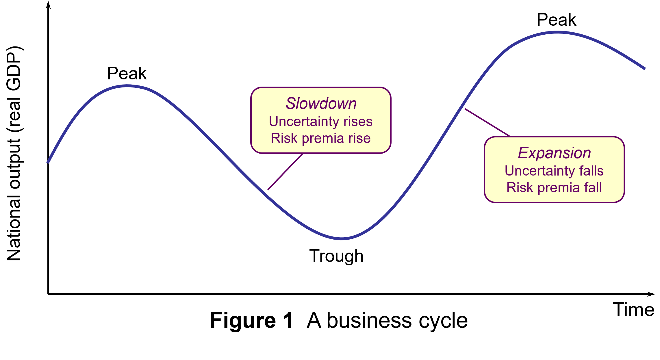
The business cycle refers to repeated sequences of expansion and contraction (or slowdown) in economic activity over time. Figure 1 illustrates a typical cycle. Typically, these sequences include four main stages. In each one there are different effects on consumer and business confidence:
- Expansion: During this stage, the economy experiences growth in GDP, with incomes and consumption spending rising. Business and consumer confidence are high. Unemployment is falling.
- Peak: This is the point at which the economy reaches its maximum output, but growth has ceased (or slowed). At this stage, inflationary pressures peak as the economy presses against potential output. This tends to result in tighter monetary policy (higher interest rates).
- Slowdown: The higher interest rates raise the cost of borrowing and reduce consumption and investment spending. Consumption and incomes both slow or fall. (Figure 1 illustrates the severe case of falling GDP (negative growth) in this stage.) Unemployment starts rising.
- Trough: This is the lowest point of the cycle, where economic activity bottoms out and the economy begins to recover. This can be associated with slow but still rising national income (a soft landing) or national income that has fallen (a hard landing, as shown in Figure 1).
While business cycles are common enough to enable such characterisation of their temporal pattern, their length and magnitude are variable and this produces great uncertainty, particularly when cycles approach peaks and troughs.
 As an economy’s cycle approaches a trough, such as US economy’s over the past few months, uncertainty is exacerbated. The high interest rates used to tackle inflation will have increased borrowing costs for businesses and consumers. Access to credit may have become more restricted. Profit margins are reduced, especially for industrial sectors sensitive to the business cycle, reducing expected cash flows.
The combination of these factors can increase the risk of a recession, producing greater volatility in financial markets. This manifests itself in increased risk aversion among investors.
Utility theory suggests that, in general, investors will exhibit loss aversion. This means that they do not like bearing risk, fearing that the return from an investment may be less than expected. In such circumstances, investors need to be compensated for bearing risk. This is normally expressed in terms of expected financial return. To bear more risk, investors require higher levels of return as compensation.
As perceptions of risk change through the business cycle, so this will change the return investors will require from the financial instruments they hold. Perceived higher risk raises the return investors will require as compensation. Conversely, lower perceived risk decreases the return investors expect as compensation.
Investors’ expected rate of return is manifested in the discount rate that they use to value the anticipated cash flows from financial instruments in discounted cash flow (DCF) analysis. Equation 1 is the algebraic expression of the present-value discounted series of cash flows for financial instruments:

Where:
V = present value
C = anticipated cash flows in each of time periods 1, 2, 3, etc.
r = expected rate of return
For fixed-income debt securities, the cash flow is constant, while for equity securities (shares), expectations regarding cash flows can change.
Slowing economies and risk aversion
 In a slowing economy, with great uncertainty about the scale and timing of the bottom of the cycle, investors become more risk averse about the prospects of firms. This this leads to higher risk premia for financial instruments sensitive to a slowdown in economic activity.
This translates into a higher expected return and higher discount rate used in the valuation of these instruments (r in equation 1). This produces decreases in perceived value, decreased demand and decreased prices for these financial instruments. This can be observed in the market dynamics for these instruments.
First, there may be a ‘flight to safety’. Investors attach a higher risk premium to risker financial instruments, such as equities, and seek a ‘safe-haven’ for their wealth. Therefore, we should observe a reorientation from more risky to less risky assets. Demand for equities falls, while demand for safer assets, such as government bonds and gold, rises.
There is some evidence for this behaviour as uncertainty about the US economic outlook has increased. Gold, long seen as a hedge against market decline, is at record highs. US Government bond prices have risen too.
To analyse whether this may be a flight to safety, I analysed the correlation between the daily US government bond price (5-year Treasury Bill) and share prices represented by the two more significant stock market indices in the USA: the S&P 500 and the Nasdaq Composite. I did this for two different time periods. Table 1 shows the results. Panel (a) shows the correlation coefficients for the period between 1 May 2024 and 31 July 2024; Panel (b) shows the correlation coefficients for the period between 1 August 2024 and 9 September 2024.
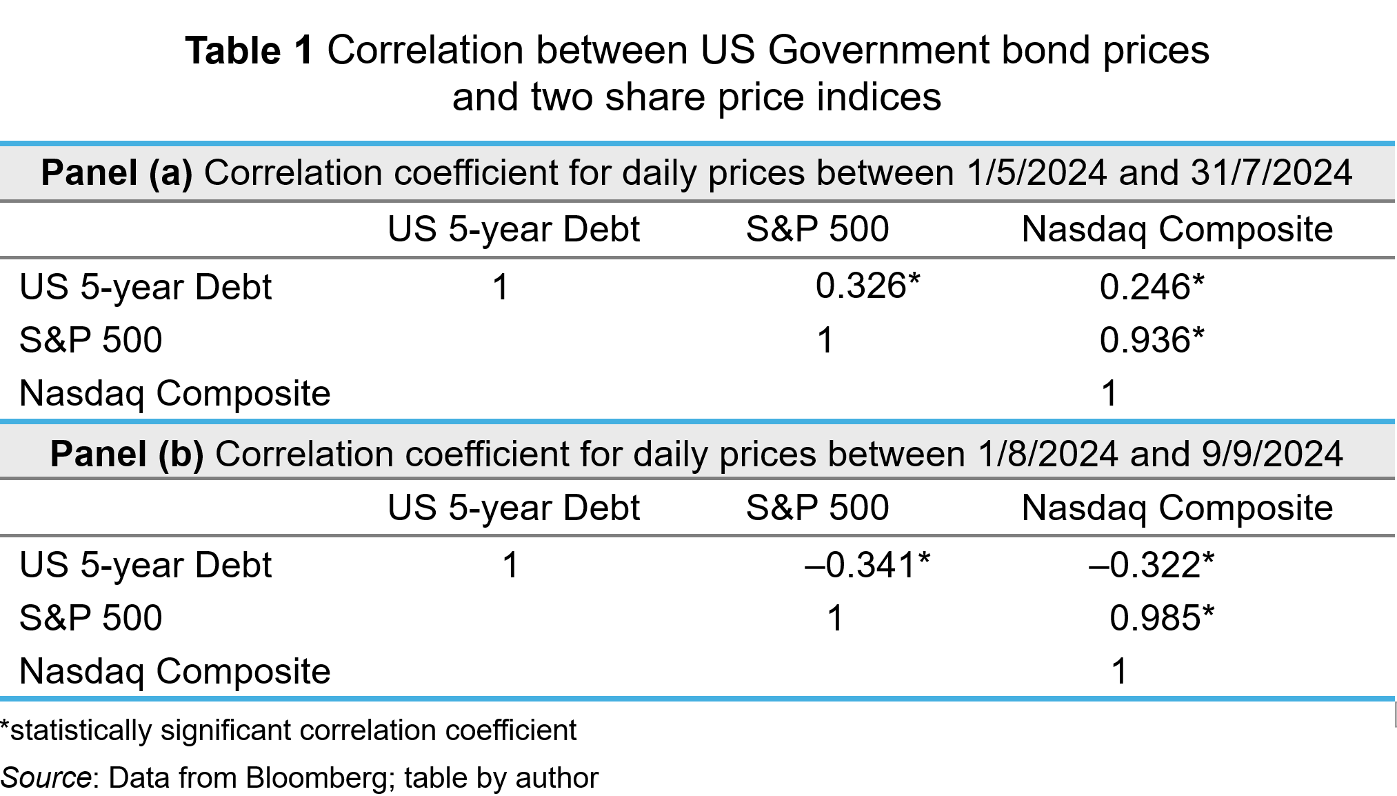
In the period between May and July 2024, the 5-year Treasury Bill and share price indices had significantly positive correlations. When share prices rose, the Treasury Bill’s price rose; when share prices fell, the bill’s price fell. During that period, expectations about falling interest rates dominated valuations and that effected the valuations of all financial instruments in the same way – lower expected interest rates reduce the opportunity cost of holding instruments and reduces the expected rates of return. Hence, the discount rate applied to cash flows is reduced, and present value rises. The opposite happens when macroeconomic indicators suggest that interest rates will stay high (ceteris paribus).
As the summer proceeded, worries about a ‘hard landing’ began to concern investors. A weak jobs report in early August particularly exercised markets, producing a ‘flight to safety’. Greater risk aversion among investors meant that they expect a higher return from equities. This reduced perceived value, reducing demand and price (ceteris paribus). To insulate themselves from higher risk, investors bought safer assets, like government bonds, thereby pushing up their prices. This behaviour was consistent with the significant negative correlation observed between US government debt prices and the S&P 500 and Nasdaq indices in Panel (b).
Another signal of increased risk aversion among investors is ‘sector rotation’ in their equity portfolios. Increased risk aversion among investors will lead them to divest from ‘cyclical’ companies. Such companies are in industrial sectors which are more sensitive to the changing economic conditions across the business cycle – consumer discretionary and communication services sectors, for example. To reduce their exposure to risk, investors will switch to ‘defensive’ sectors – those less sensitive to the business cycle. Examples include consumer staples and utility sectors.
Cyclical sectors will suffer a greater adverse impact on their cash flows and risk in a slowing economy. Consequently, investors expect higher return as compensation. This reduces the value of those shares. Demand for them falls, depressing their price. In contrast, defensive sectors will be valued more. They will see an increase in demand and price. This sector rotation seems to have happened in August (2024). Figure 2 shows the percentage change between 1 August and 9 September 2024 in the S&P 500 index and four sector indices, comprising companies from the communication services, consumer discretionary, consumer staples and utilities sectors.
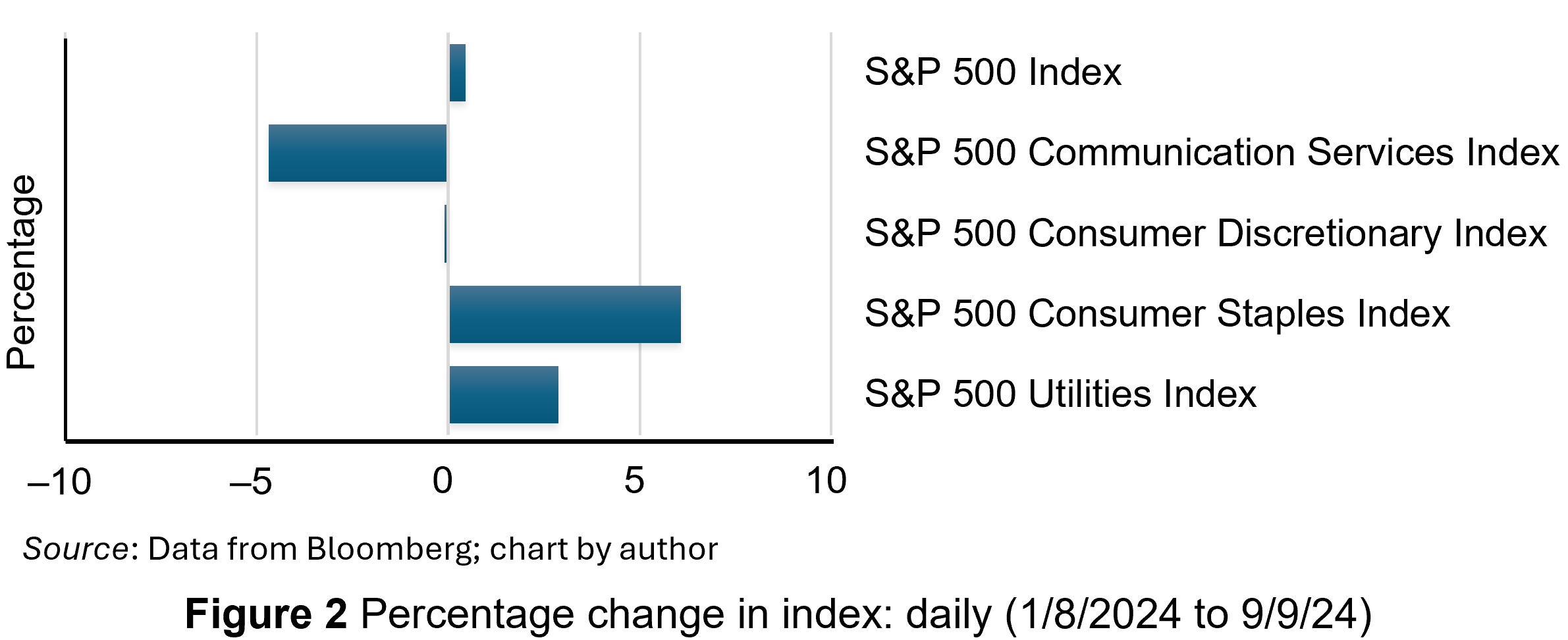
Overall, the S&P 500 index was slightly higher, as shown by the first bar in the chart. However, while the cyclical sectors experienced decreases in their share prices, particularly communication services, the defensive companies experienced large price increases – nearly 3% for utilities and over 6% for consumer staples.
Conclusion
Economies experience repeated sequences of expansion and contraction in economic activity over time. At the moment, the US economy is approaching the end of its current slowing phase. Increased uncertainty is a common feature of late-cycle economies and this manifests itself in heightened risk aversion among investors. This produces certain dynamics which have been observable in US debt and equity markets. This includes a ‘flight to safety’, with investors divesting risky financial instruments in favour of safer ones, such as US government debt securities and gold. Also, investors have been reorientating their equity portfolios away from cyclicals and towards defensive securities.
Articles
- America’s recession signals are flashing red. Don’t believe them
The Economist (22/8/24)
- The most well-known recession indicator stopped flashing red, but now another one is going off
CNN, Elisabeth Buchwald (13/9/24)
- World’s largest economy will still achieve soft landing despite rising unemployment, most analysts believe
Financial Times, Claire Jones, Delphine Strauss and Martha Muir (6/8/24)
- We’re officially on slowdown watch
Financial Times, Robert Armstrong and Aiden Reiter (30/8/24)
- Anatomy of a rout
Financial Times, Robert Armstrong and Aiden Reiter (6/8/24)
- Reasons why investors need to prepare for a US recession
Financial Times, Peter Berezin (5/9/24)
- Business Cycle: What It Is, How to Measure It, and Its 4 Phases
Investopedia, Lakshman Achuthan (6/6/24)
- Risk Averse: What It Means, Investment Choices, and Strategies
Investopedia, James Chen (5/8/24)
Data
Questions
- What is risk aversion? Sketch an indifference curve for a risk-averse investor, treating expected return and risk as two-characteristics of a financial instrument.
- Show what happens to the slope of the indifference curve if the investor becomes more risk averse.
- Using demand and supply analysis, illustrate and explain the impact of a flight to safety on the market for (i) company shares and (ii) US government Treasury Bills.
- Use economic theory to explain why the consumer discretionary sector may be more sensitive than the consumer staples sector to varying incomes across the economic cycle.
- Research the point of the economic cycle that the US economy has reached as you read this blog. What is the relationship between bond and equity prices? Which sectors have performed best in the stock market?
 To finance budget deficits, governments have to borrow. They can borrow short-term by issuing Treasury bills, typically for 1, 3 or 6 months. These do not earn interest and hence are sold at a discount below the face value. The rate of discount depends on supply and demand and will reflect short-term market rates of interest. Alternatively, governments can borrow long-term by issuing bonds. In the UK, these government securities are known as ‘gilts’ or ‘gilt-edged securities’. In the USA they are known as ‘treasury bonds’, ‘T-bonds’ or simply ‘treasuries’. In the EU, countries separately issue bonds but the European Commission also issues bonds.
In the UK, gilts are issued by the Debt Management Office on behalf of the Treasury. Although there are index-linked gilts, the largest proportion of gilts are conventional gilts. These pay a fixed sum of money per annum per £100 of face value. This is known as the ‘coupon payment’ and the rate is set at the time of issue. The ‘coupon rate’ is the payment per annum as a percentage of the bond’s face value:

Payments are made six-monthly. Each issue also has a maturity date, at which point the bonds will be redeemed at face value. For example, a 4½% Treasury Gilt 2028 bond has a coupon rate of 4½% and thus pays £4.50 per annum (£2.25 every six months) for each £100 of face value. The issue will be redeemed in June 2028 at face value. The issue was made in June 2023 and thus represented a 5-year bond. Gilts are issued for varying lengths of time from 2 to 55 years. At present, there are 61 different conventional issues of bonds, with maturity dates varying from January 2024 to October 2073.
Bond prices
 Bonds can be sold on the secondary market (i.e. the stock market) before maturity. The market price, however, is unlikely to be the coupon price (i.e. the face value). The lower the coupon rate relative to current interest rates, the less valuable the bond will be. For example, if interest rates rise, and hence new bonds pay a higher coupon rate, the market price of existing bonds paying a lower coupon rate must fall. Thus bond prices vary inversely with interest rates.
The market price also depends on how close the bonds are to maturity. The closer the maturity date, the closer the market price of the bond will be to the face value.
Bond yields: current yield
A bond’s yield is the percentage return that a person buying the bond receives. If a newly issued bond is bought at the coupon price, its yield is the coupon rate.
However, if an existing bond is bought on the secondary market (the stock market), the yield must reflect the coupon payments relative to the purchase price, not the coupon price. We can distinguish between the ‘current yield’ and the ‘yield to maturity’.
The current yield is the coupon payment as a percentage of the current market price of the bond:

Assume a bond were originally issued at 2% (its coupon rate) and thus pays £2 per annum. In the meantime, however, assume that interest rates have risen and new bonds now have a coupon rate of 4%, paying £4 per annum for each £100 invested. To persuade people to buy old bonds with a coupon rate of 2%, their market prices must fall below their face value (their coupon price). If their price halved, then they would pay £2 for every £50 of their market price and hence their current yield would be 4% (£2/£50 × 100).
Bond yields: yield to maturity (YTM)
But the current yield does not give the true yield – it is only an approximation. The true yield must take into account not just the market price but also the maturity value and the length of time to maturity (and the frequency of payments too, which we will ignore here). The closer a bond is to its maturity date, the higher/lower will be the true yield if the price is below/above the coupon price: in other words, the closer will the market price be to the coupon price for any given market rate of interest.
A more accurate measure of a bond’s yield is thus the ‘yield to maturity’ (YTM). This is the interest rate which makes the present value of all a bond’s future cash flows equal to its current price. These cash flows include all coupon payments and the payment of the face value on maturity. But future cash flows must be discounted to take into account the fact that money received in the future is worth less than money received now, since money received now could then earn interest.
The yield to maturity is the internal rate of return (IRR) of the bond. This is the discount rate which makes the present value (PV) of all the bond’s future cash flows (including the maturity payment of the coupon price) equal to its current market price. For simplicity, we assume that coupon payments are made annually. The formula is the one where the bond’s current market price is given by:

Where: t is the year; n is the number of years to maturity; YTM is the yield to maturity.
Thus if a bond paid £5 each year and had a maturity value of £100 and if current interest rates were higher than 5%, giving a yield to maturity of 8%, then the bond price would be:

In other words, with a coupon rate of 5% and a higher YTM of 8%, the bond with a face value of £100 and five years to maturity would be worth only £88.02 today.
If you know the market price of a given bond, you can work out its YTM by substituting in the above formula. The following table gives examples.
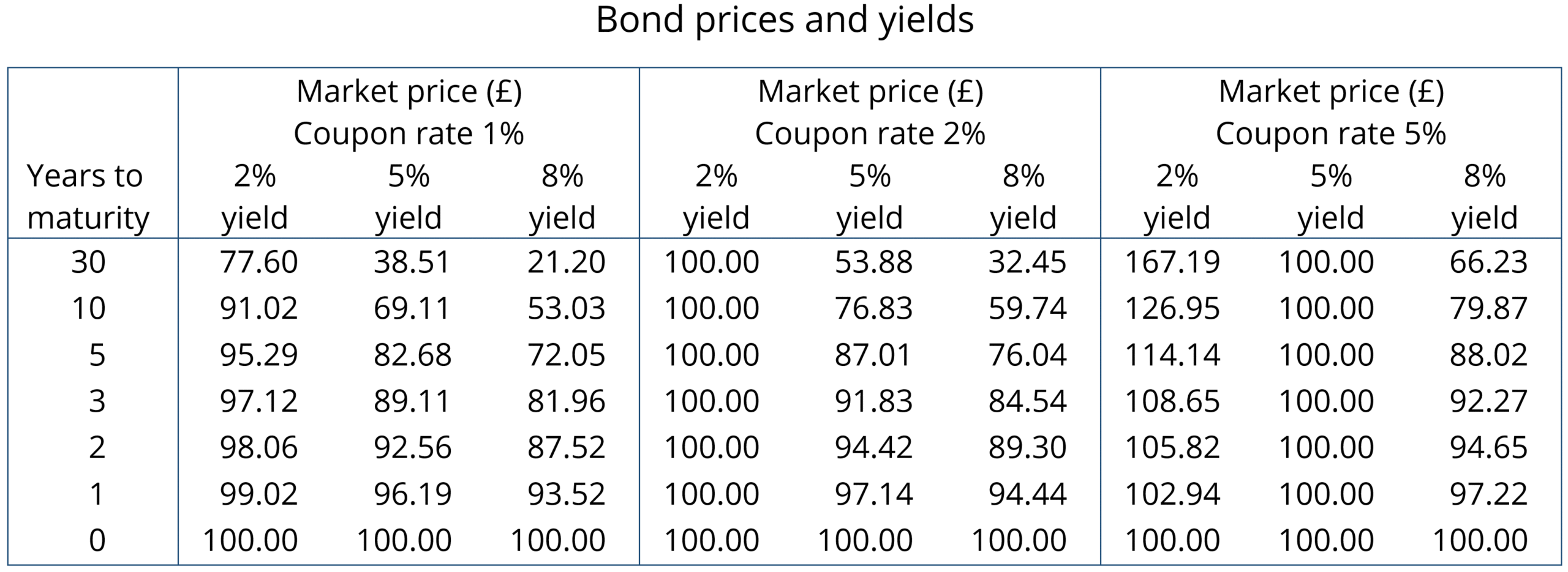
The higher the YTM, the lower the market price of a bond. Since the YTM reflects in part current rates of interest, so the higher the rate of interest, the lower the market price of any given bond. Thus bond yields vary directly with interest rates and bond prices vary inversely. You can see this clearly from the table. You can also see that market bond prices converge on the face value as the maturity date approaches.
Recent activity in bond markets
Investing in government bonds is regarded as very safe. Coupon payments are guaranteed, as is repayment of the face value on the maturity date. For this reason, many pension funds hold a lot of government bonds issued by financially trustworthy governments. But in recent months, bond prices in the secondary market have fallen substantially as interest rates have risen. For those holding existing bonds, this means that their value has fallen. For governments wishing to borrow by issuing new bonds, the cost has risen as they have to offer a higher coupon rate to attract buyers. This make it more expensive to finance government debt.
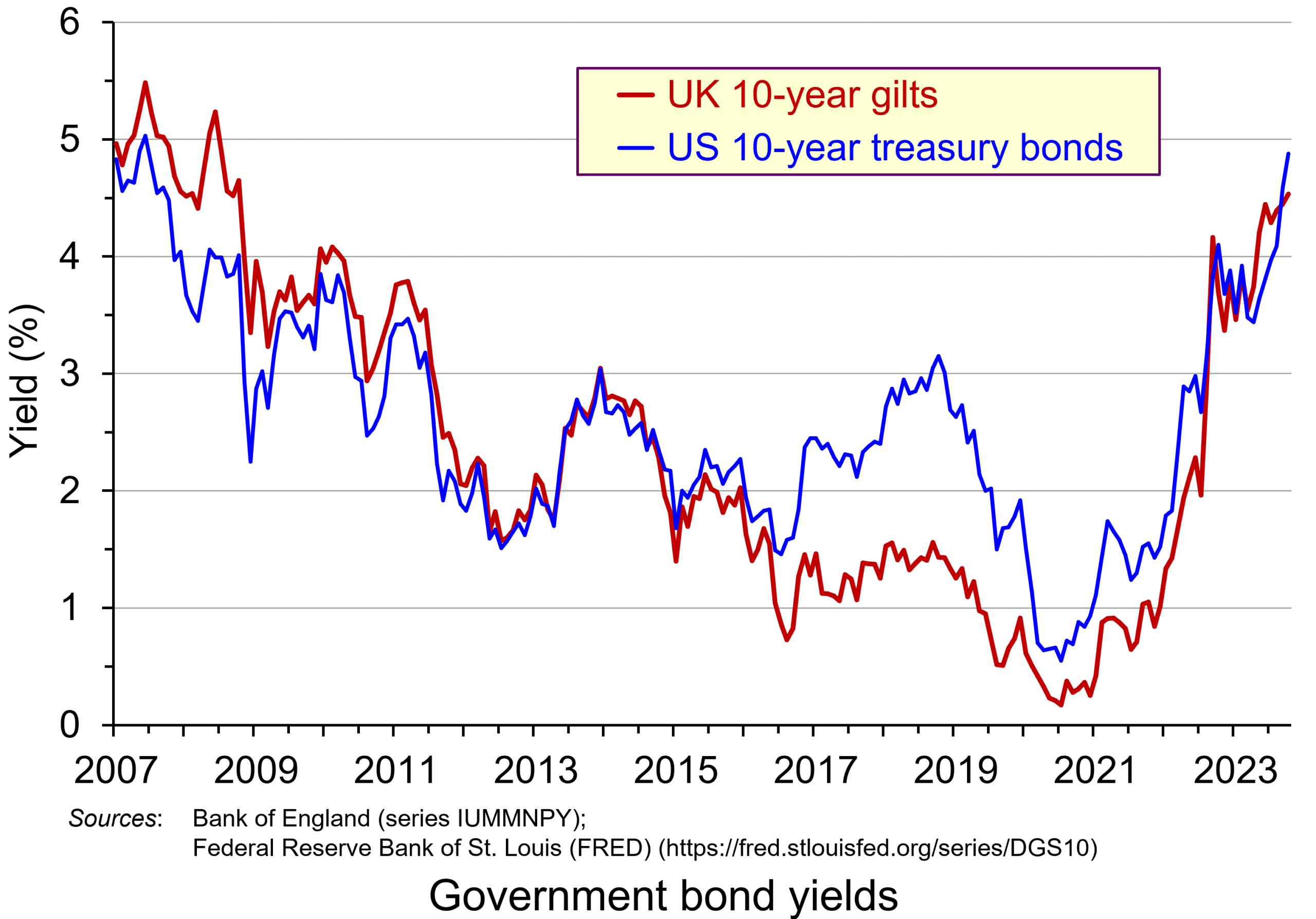 The chart shows the yield on 10-year government bonds. It is calculated using the ‘par value’ approach. This gives the coupon rate that would have to be paid for the market price of a bond to equal its face value. Clearly, as interest rates rise, a bond would have to pay a higher coupon rate for this to happen. (This, of course, is only hypothetical to give an estimate of market rates, as coupon rates are fixed at the time of a bond’s issue.)
Par values reflect both yield to maturity and also expectations of future interest rates. The higher people expect future interest rates to be, the higher must par values be to reflect this.
 In the years following the financial crisis of 2007–8 and the subsequent recession, and again during the COVID pandemic, central banks cut interest rates and supported this by quantitative easing. This involved central banks buying existing bonds on the secondary market and paying for them with newly created (electronic) money. This drove up bond prices and drove down yields (as the chart shows). This helped support the policy of low interest rates. This was a boon to governments, which were able to borrow cheaply.
This has all changed. With quantitative tightening replacing quantitative easing, central banks have been engaging in asset sales, thereby driving down bond prices and driving up yields. Again, this can be seen in the chart. This has helped to support a policy of higher interest rates.
Problems of higher bond yields/lower bond prices
Although lower bond prices and higher yields have supported a tighter monetary policy, which has been used to fight inflation, this has created problems.
First, it has increased the cost of financing government debt. In 2007/8, UK public-sector net debt was £567bn (35.6% of GDP). The Office for Budget Responsibility forecasts that it will be £2702bn (103.1% of GDP in the current financial year – 2023/24). Not only, therefore, are coupon rates higher for new government borrowing, but the level of borrowing is now a much higher proportion of GDP. In 2020/21, central government debt interest payments were 1.2% of GDP; by 2022/23, they were 4.4% (excluding interest on gilts held in the Bank of England, under the Asset Purchase Facility (quantitative easing)).
 In the USA, there have been similar increases in government debt and debt interest payments. Debt has increased from $9tn in 2007 to $33.6tn today. Again, with higher interest rates, debt interest as a percentage of GDP has risen: from 1.5% of GDP in 2021 to a forecast 2.5% in 2023 and 3% in 2024. What is more, 31 per cent of US government bonds will mature next year and will need refinancing – at higher coupon rates.
There is a similar picture in other developed countries. Clearly, higher interest payments leave less government revenue for other purposes, such as health and education.
Second, many pension funds, banks and other investment companies hold large quantities of bonds. As their price falls, so this reduces the value of these companies’ assets and makes it harder to finance new purchases, or payments or loans to customers. However, the fact that new bonds pay higher interest rates means that when existing bond holdings mature, the money can be reinvested at higher rates.
Third, bonds are often used by companies as collateral against which to borrow and invest in new capital. As bond prices fall, this can hamper companies’ ability to invest, which will lead to lower economic growth.
Fourth, higher bond yields divert demand away from equities (shares). With equity markets falling back or at best ceasing to rise, this erodes the value of savings in equities and may make it harder for firms to finance investment through new issues.
At the core of all these problems is inflation and budget deficits. Central banks have responded by raising interest rates. This drives up bond yields and drives down bond prices. But bond prices and yields depend not just on current interest rates, but also on expectations about future interest rates. Expectations currently are that budget deficits will be slow to fall as governments seek to support their economies post-COVID. Also expectations are that inflation, even though it is falling, is not falling as fast as originally expected – a problem that could be exacerbated if global tensions increase as a result of the ongoing war in Ukraine, the Israel/Gaza war and possible increased tensions with China concerning disputes in the China Sea and over Taiwan. Greater risks drive up bond yields as investors demand a higher interest premium.
Articles
Information and data
Questions
- Why do bond prices and bond yields vary inversely?
- How are bond yields and prices affected by expectations?
- Why are ‘current yield’ and ‘yield to maturity’ different?
- What is likely to happen to bond prices and yields in the coming months? Explain your reasoning.
- What constraints do bond markets place on fiscal policy?
- Would it be desirable for central banks to pause their policy of quantitative tightening?
 Over the decades, economies have become increasingly interdependent. This process of globalisation has involved a growth in international trade, the spread of technology, integrated financial markets and international migration.
When the global economy is growing, globalisation spreads the benefits around the world. However, when there are economic problems in one part of the world, this can spread like a contagion to other parts. This was clearly illustrated by the credit crunch of 2007–8. A crisis that started in the sub-prime market in the USA soon snowballed into a worldwide recession. More recently, the impact of Covid-19 on international supply chains has highlighted the dangers of relying on a highly globalised system of production and distribution. And more recently still, the war in Ukraine has shown the dangers of food and fuel dependency, with rapid rises in prices of basic essentials having a disproportionate effect on low-income countries and people on low incomes in richer countries.
Moves towards autarky
So is the answer for countries to become more self-sufficient – to adopt a policy of greater autarky? Several countries have moved in this direction. The USA under President Trump pursued a much more protectionist agenda than his predecessors. The UK, although seeking new post-Brexit trade relationships, has seen a reduction in trade as new barriers with the EU have reduced UK exports and imports as a percentage of GDP.  According to the Office for Budget Responsibility’s November 2022 Economic and Fiscal Outlook, Brexit will result in the UK’s trade intensity being 15 per cent lower in the long run than if it had remained in the EU.
Many European countries are seeking to achieve greater energy self-sufficiency, both as a means of reducing reliance on Russian oil and gas, but also in pursuit of a green agenda, where a greater proportion of energy is generated from renewables. More generally, countries and companies are considering how to reduce the risks of relying on complex international supply chains.
Limits to the gains from trade
The gains from international trade stem partly from the law of comparative advantage, which states that greater levels of production can be achieved by countries specialising in and exporting those goods that can be produced at a lower opportunity cost and importing those in which they have a comparative disadvantage. Trade can also lead to the transfer of technology and a downward pressure on costs and prices through greater competition.
 But trade can increase dependence on unreliable supply sources. For example, at present, some companies are seeking to reduce their reliance on Taiwanese parts, given worries about possible Chinese actions against Taiwan.
Also, governments have been increasingly willing to support domestic industries with various non-tariff barriers to imports, especially since the 2007–8 financial crisis. Such measures include subsidies, favouring domestic firms in awarding government contracts and using regulations to restrict imports. These protectionist measures are often justified in terms of achieving security of supply. The arguments apply particularly starkly in the case of food. In the light of large price increases in the wake of the Ukraine war, many countries are considering how to increase food self-sufficiency, despite it being more costly.
Also, trade in goods involves negative environmental externalities, as freight transport, whether by sea, air or land, involves emissions and can add to global warming. In 2021, shipping emitted over 830m tonnes of CO2, which represents some 3% of world total CO2 emissions. In 2019 (pre-pandemic), the figure was 800m tonnes. The closer geographically the trading partner, the lower these environmental costs are likely to be.
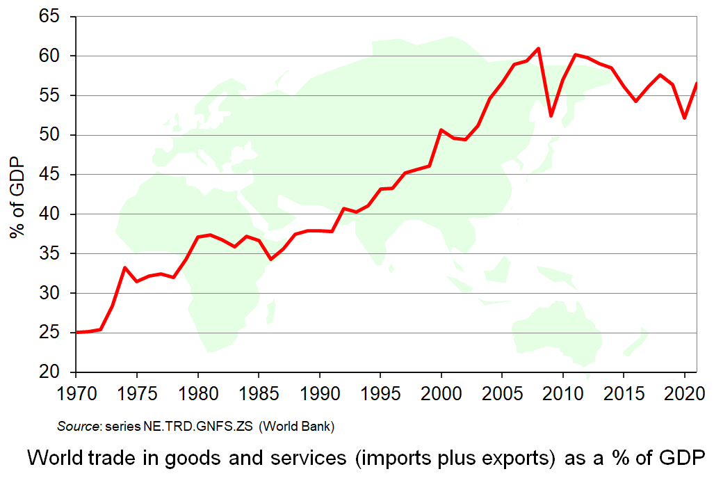 The problems with a globally interdependent world have led to world trade growing more slowly than world GDP in recent years after decades of trade growth considerably outstripping GDP growth. Trade (imports plus exports) as a percentage of GDP peaked at just over 60% in 2008. In 2019 and 2021 it was just over 56%. This is illustrated in the chart (click here for a PowerPoint). Although trade as a percentage of GDP rose slightly from 2020 to 2021 as economies recovered from the pandemic, it is expected to have fallen back again in 2022 and possibly further in 2023.
But despite this reduction in trade as a percentage of GDP, with de-globalisation likely to continue for some time, the world remains much more interdependent than in the more distant past (as the chart shows). Greater autarky may be seen as desirable by many countries as a response to the greater economic and political risks of the current world, but greater autarky is a long way from complete self-sufficiency. The world is likely to remain highly interdependent for the foreseeable future. Reports of the ‘death of globalisation’ are premature!
Podcasts
Articles
Report
Questions
- Explain the law of comparative advantage and demonstrate how trade between two countries can lead to both countries gaining.
- What are the main economic problems arising from globalisation?
- Is the answer to the problems of globalisation to move towards greater autarky?
- Would the expansion/further integration of trading blocs be a means of exploiting the benefits of globalisation while reducing the risks?
- Is the role of the US dollar likely to decline over time and, if so, why?
- Summarise Karl Polanyi’s arguments in The Great Transformation (see the Daniel W. Drezner article linked below). How well do they apply to the current world situation?
 Mid-December saw a rapid rise in coronavirus cases in London and the South East and parts of eastern and central southern England. This was due to a new strain of Covid, which is more infectious. In response, the UK government introduced a new tier 4 level of restrictions for these areas from 20 December. These amount to a complete lockdown. The devolved administrations also announced lockdowns. In addition, the Christmas relaxation of rules was tightened across the UK. Households (up to three) were only allowed to get together on Christmas day and not the days either side (or one day between 23 and 27 December in the case of Northern Ireland). Tier 4 residents were not allowed to visit other households even on Christmas day.
The lockdowns aimed to slow the spread of the virus and reduce deaths. But this comes at a considerable short-term economic cost, especially to the retail and leisure sectors, which are required to close while the lockdowns remain in force. In taking the decision to introduce these tougher measures, the four administrations had to weigh up the benefits of reduced deaths and illness and pressure on the NHS against the short-term economic damage. As far a long-term economic damage is concerned, this might be even greater if lockdowns were not imposed and the virus spread more rapidly.
In a blog back in September, we examined the use of cost–benefit analysis (CBA) to aid decision-making about such decisions. The following is an updated version of that blog.
The use of cost–benefit analysis
 It is commonplace to use cost–benefit analysis (CBA) in assessing public policies, such as whether to build a new hospital, road or rail line. Various attempts in the past few months have been made to use CBA in assessing policies to reduce the spread of the coronavirus. These have involved weighing up the costs and benefits of national or local lockdowns or other containment measures. But, as with other areas where CBA is used, there are serious problems of measuring costs and benefits and assessing risks. This is particularly problematic where human life is involved and where a value has to be attached to a life saved or lost.
The first step in a CBA is to identify the benefits and costs of the policy.
Identifying the benefits and costs of the lockdown
The benefits of the lockdown include lives saved and a reduction in suffering, not only for those who otherwise would have caught the virus but also for their family and friends. It also includes lives saved from other diseases whose treatment would have been put (even more) on hold if the pandemic had been allowed to rage and more people were hospitalised with the virus. In material terms, there is the benefit of saving in healthcare and medicines and the saving of labour resources. Then there are the environmental gains from less traffic and polluting activities.
 On the cost side, there is the decline in output from businesses being shut and people being furloughed or not being able to find work. There is also a cost if schools have to close and children’s education is thereby compromised. Then there is the personal cost to people of being confined to home, a cost that could be great for those in cramped living conditions or in abusive relationships. Over the longer term, there is a cost from people becoming deskilled and firms not investing – so-called scarring effects. Here there are the direct effects and the multiplier effects on the rest of the economy.
Estimating uncertain outcomes
 It is difficult enough identifying all the costs and benefits, but many occur in the future and here there is the problem of estimating the probability of their occurrence and their likely magnitude. Just how many lives will be saved from the policy and just how much will the economy be affected? Epidemiological and economic models can help, but there is a huge degree of uncertainty over predictions made about the spread of the disease, especially with a new strain of the virus, and the economic effects, especially over the longer term.
One estimate of the number of lives saved was made by Miles et al. in the NIESR paper linked below. A figure of 440 000 was calculated by subtracting the 60 000 actual excess deaths over the period of the first lockdown (March to June 2020) from a figure of 500 000 lives lost which, according to predictions, would have been the consequence of no lockdown. However, the authors acknowledge that this is likely to be a considerable overestimate because:
It does not account for changes in behaviour that would have occurred without the government lockdown; it does not count future higher deaths from side effects of the lockdown (extra cancer deaths for example); and it does not allow for the fact that some of those ‘saved’ deaths may just have been postponed because when restrictions are eased, and in the absence of a vaccine or of widespread immunity, deaths may pick up again.
Some help in estimating likely outcomes from locking down or not locking down the economy can be gained by comparing countries which have taken different approaches. The final article in the first list below compares the approaches in the UK and Sweden. Sweden had much lighter control measures than the UK and did not impose a lockdown. Using comparisons of the two approaches, the authors estimate that some 20 000 lives were saved by the lockdown – considerably less than the 440 000 estimate.
Estimating the value of a human life
To assess whether the saving of 20 000 lives was ‘worth it’, a value would have to be put on a life saved. Although putting a monetary value on a human life may be repugnant to many people, such calculations are made whenever a project is assessed which either saves or costs lives. As we say in the 10th edition of Economics (page 381):
Some people argue ‘You can’t put a price on a human life: life is priceless.’ But just what are they saying here? Are they saying that life has an infinite value? If so, the project must be carried out whatever the costs, and even if other benefits are zero! Clearly, when evaluating lives saved from the project, a value less than infinity must be given.
Other people might argue that human life cannot be treated like other costs and benefits and put into mathematical calculations. But what are these people saying? That the question of lives saved should be excluded from the cost–benefit study? If so, the implication is that life has a zero value! Again this is clearly not the case.
In practice, there are two approaches used to measure the value of a human life.
 The first uses the value of a statistical life (VSL). This is based on the amount extra the average person would need to be paid to work in a job where there is a known probability of losing their life. So if people on average needed to be paid an extra £10 000 to work in a job with a 1% chance of losing their life, they would be valuing a life at £1 000 000 (£10 000/0.01). To avoid the obvious problem of young people’s lives being valued the same as old people’s ones, even though a 20 year-old on average will live much longer than a 70 year-old, a more common measure is the value of a statistical life year (VSLY).
A problem with VSL or VSLY measures is that they only take into account the quantity of years of life lost or saved, not the quality.
A second measure rectifies this problem. This is the ‘quality of life adjusted year (QALY)’. This involves giving a value to a year of full health and then reducing it according to how much people’s quality of life is reduced by illness, injury or poverty. The problem with this measure is the moral one that a sick or disabled person’s life is being valued less than the life of a healthy person. But it is usual to make such adjustments when considering medical intervention with limited resources.
One adjustment often made to QALYs or VSLYs is to discount years, so that one year gained would be given the full value and each subsequent year would be discounted by a certain percentage from the previous year – say, 3%. This would give a lower weighting to years in the distant future than years in the near future and hence would reduce the gap in predicted gains from a policy between young and old people.
Cost–effectiveness analysis (CEA)
Even using QALYs, there is still the problem of measuring life and health/sickness. A simpler approach is to use cost–effectiveness analysis (CEA). This takes a social goal, such as reducing the virus production rate (R) below 1 (e.g. to 0.9), and then finding the least-cost way of achieving this. As Mark Carney says in his third Reith Lecture:
As advocated by the economists Nick Stern and Tim Besley, the ideal is to define our core purpose first and then determine the most cost-effective interventions to achieve this goal. Such cost–effectiveness analysis explicitly seeks to achieve society’s values.
Cost–effectiveness analysis can take account of various externalities – as many of the costs will be – by giving them a value. For example, the costs of a lockdown to people in the hospitality sector or to the education of the young could be estimated and included in the costs. The analysis can also take into account issues of fairness by identifying the effects on inequality when certain groups suffer particularly badly from Covid or lockdown policies – groups such as the poor, the elderly and children. Achieving the goal of a specific R for the least cost, including external costs and attaching higher weights on the effects on certain groups then becomes the goal. As Carney says:
R brings public health and economics together. Relaxations of restrictions increase R, with economic, health and social consequences. A strategic approach to Covid is the best combination of policies to achieve the desired level of infection control at minimum economic cost with due respect for inequality, mental health and other social consequences, and calculating those costs then provides guidance when considering different containment strategies. That means paying attention to the impact on measures of fairness, the social returns to education, intergenerational equity and economic dynamism.
Conclusion
Given the uncertainties surrounding the measurement of the number of lives saved and the difficulties of assigning a value to them, and given the difficulties of estimating the economic and social effects of lockdowns, it is not surprising that the conclusions of a cost–benefit analysis, or even a cost–effectiveness analysis of a lockdown will be contentious. But, at least such analysis can help to inform discussion and drive future policy decisions. And a cost–effectiveness analysis can be a practical way of helping politicians reach difficult decisions about life and death and the economy.
Articles (original blog)
- When Does the Cure Become Worse Than the Disease? Applying Cost-Benefit Analysis to the Covid-19 Recovery
Journal of Medical Ethics, blog, Derek Soled, Michelle Bayefsky and Rahul Nayak (19/5/20)
- How much did the Covid-19 lockdown really cost the UK?
The Guardian, Larry Elliott (6/9/20)
- The UK lockdown: Balancing costs against benefits
VoxEU, David Miles (13/7/20)
- How Economists Calculate The Costs And Benefits Of COVID-19 Lockdowns
Forbes, Chris Conover (27/3/20)
- Coronavirus Is Giving Cost-Benefit Analysts Fits
Bloomberg, Cass R. Sunstein (12/5/20)
- “Stay at Home, Protect the National Health Service, Save Lives”: a cost benefit analysis of the lockdown in the United Kingdom
Wiley Online Library, David Miles, Mike Stedman and Adrian Heald (13/8/20)
- COVID-19 is Forcing Economists to Rethink the Value of Life
RealClearPolicy, James Broughel (20/8/20)
- A cost–benefit analysis of the COVID-19 disease
Oxford Review of Economic Policy, Robert Rowthorn and Jan Maciejowski (28/8/20)
- Living with Covid-19: Balancing Costs against Benefits in the Face of the Virus
National Institute Economic Review, vol. 253, David Miles, Mike Stedman and Adrian Heald (28/7/20)
- How Many Lives Has Lockdown Saved in the UK?
medRxiv, Rickard Nyman and Paul Ormerod (21/8/20)
Articles (additional)
Questions
- What are the arguments for and against putting a monetary value on a life saved?
- Are QALYs the best way of measuring lives saved from a policy such as a lockdown?
- Compare the relative merits of cost–benefit analysis and cost–effectiveness analysis.
- If the outcomes of a lockdown are highly uncertain, does this strengthen or weaken the case for a lockdown? Explain.
- What specific problems are there in estimating the number of lives saved by a lockdown?
- How might the age distribution of people dying from Covid-19 affect the calculation of the cost of these deaths (or the benefits or avoiding them)?
- How might you estimate the costs to people who suffer long-term health effects from having had Covid-19?
- What are the arguments for and against using discounting in estimating future QALYs?
- The Department of Transport currently uses a figure of £1 958 303 (in 2018 prices) for the value of a life saved from a road safety project. Find out how this is figure derived and comment on it. See Box 12.5 in Economics 10th edition and Accident and casualty costs, Tables RAS60001 and RA60003, (Department of Transport, 2019).
 We continue to live through incredibly turbulent times. In the past decade or so we have experienced a global financial crisis, a global health emergency, seen the UK’s departure from the European Union, and witnessed increasing levels of geopolitical tension and conflict. Add to this the effects from the climate emergency and it easy to see why the issue of economic uncertainty is so important when thinking about a country’s economic prospects.
 Figure 1 (click here for a PowerPoint) shows the WUI both globally and in the UK quarterly since 1991. The global index covers 143 countries and is presented as both a simple average and a GDP weighted average. The UK WUI is also shown. This is a three-quarter weighted average, the authors’ preferred measure for individual countries, where increasing weights of 0.1, 0.3 and 0.6 are used for the three most recent quarters.
 As Figure 2 shows (click here for a PowerPoint), investment is particularly volatile, and much more so than household spending. Some of this can be attributed to the ‘lumpiness’ of investment decisions since these expenditures tend to be characterised by indivisibility and irreversibility. This means that they are often relatively costly to finance and are ‘all or nothing’ decisions. In the context of uncertainty, it can make sense therefore for firms to wait for news that makes the future clearer. In this sense, we can think of uncertainty rather like a fog that firms are peering through. The thicker the fog, the more uncertain the future and the more cautious firms are likely to be.
  The theory of buffer-stock saving was popularised by Christopher Carroll in 1992 (see link below). It implies that in the presence of uncertainty, people are prepared to consume less today in order to increase levels of saving, pay off existing debts, or borrow less relative to that in the absence of uncertainty. The extent of the buffer of financial wealth that people want to hold will depend on their own appetite for risk, the level of uncertainty, and the moderating effect from their own impatience and, hence, present bias for consuming today.
 Figure 3 suggests that the relationship between confidence and uncertainty is rather more complex than perhaps is generally understood (click here for a PowerPoint). Haddow, Hare, Hooley and Shakir (see link below) argue that the evidence tends to point to changes in uncertainty affecting confidence, but with less evidence that changes in confidence affect uncertainty.
 In recent months there has been growing uncertainty across the global economy as to whether the US economy was going to experience a ‘hard’ or ‘soft landing’ in the current business cycle – the repeated sequences of expansion and contraction in economic activity over time. Announcements of macroeconomic indicators have been keenly anticipated for signals about how quickly the US economy is slowing.
 As an economy’s cycle approaches a trough, such as US economy’s over the past few months, uncertainty is exacerbated. The high interest rates used to tackle inflation will have increased borrowing costs for businesses and consumers. Access to credit may have become more restricted. Profit margins are reduced, especially for industrial sectors sensitive to the business cycle, reducing expected cash flows.
 In a slowing economy, with great uncertainty about the scale and timing of the bottom of the cycle, investors become more risk averse about the prospects of firms. This this leads to higher risk premia for financial instruments sensitive to a slowdown in economic activity.

 To finance budget deficits, governments have to borrow. They can borrow short-term by
  Bonds can be sold on the secondary market (i.e. the stock market) before maturity. The market price, however, is unlikely to be the coupon price (i.e. the face value). The lower the coupon rate relative to current interest rates, the less valuable the bond will be. For example, if interest rates rise, and hence new bonds pay a higher coupon rate, the market price of existing bonds paying a lower coupon rate must fall. Thus bond prices vary inversely with interest rates.


 The chart shows the yield on 10-year government bonds. It is calculated using the ‘par value’ approach. This gives the coupon rate that would have to be paid for the market price of a bond to equal its face value. Clearly, as interest rates rise, a bond would have to pay a higher coupon rate for this to happen. (This, of course, is only hypothetical to give an estimate of market rates, as coupon rates are fixed at the time of a bond’s issue.)
  In the years following the financial crisis of 2007–8 and the subsequent recession, and again during the COVID pandemic, central banks cut interest rates and supported this by quantitative easing. This involved central banks buying existing bonds on the secondary market and paying for them with newly created (electronic) money. This drove up bond prices and drove down yields (as the chart shows). This helped support the policy of low interest rates. This was a boon to governments, which were able to borrow cheaply.
 In the USA, there have been similar increases in government debt and debt interest payments. Debt has increased from $9tn in 2007 to $33.6tn today. Again, with higher interest rates, debt interest as a percentage of GDP has risen: from 1.5% of GDP in 2021 to a forecast 2.5% in 2023 and 3% in 2024. What is more, 31 per cent of US government bonds will mature next year and will need refinancing – at higher coupon rates.
 Over the decades, economies have become increasingly interdependent. This process of globalisation has involved a growth in international trade, the spread of technology, integrated financial markets and international migration.
 According to the Office for Budget Responsibility’s November 2022 Economic and Fiscal Outlook, Brexit will result in the UK’s trade intensity being 15 per cent lower in the long run than if it had remained in the EU.
  But trade can increase dependence on unreliable supply sources. For example, at present, some companies are seeking to reduce their reliance on Taiwanese parts, given worries about possible Chinese actions against Taiwan.
  The problems with a globally interdependent world have led to world trade growing more slowly than world GDP in recent years after decades of trade growth considerably outstripping GDP growth. Trade (imports plus exports) as a percentage of GDP peaked at just over 60% in 2008. In 2019 and 2021 it was just over 56%. This is illustrated in the chart (click
 Mid-December saw a rapid rise in coronavirus cases in London and the South East and parts of eastern and central southern England. This was due to a new strain of Covid, which is more infectious. In response, the UK government introduced a new
  It is commonplace to use cost–benefit analysis (CBA) in assessing public policies, such as whether to build a new hospital, road or rail line. Various attempts in the past few months have been made to use CBA in assessing policies to reduce the spread of the coronavirus. These have involved weighing up the costs and benefits of national or local lockdowns or other containment measures. But, as with other areas where CBA is used, there are serious problems of measuring costs and benefits and assessing risks. This is particularly problematic where human life is involved and where a value has to be attached to a life saved or lost.
 On the cost side, there is the decline in output from businesses being shut and people being furloughed or not being able to find work. There is also a cost if schools have to close and children’s education is thereby compromised. Then there is the personal cost to people of being confined to home, a cost that could be great for those in cramped living conditions or in abusive relationships. Over the longer term, there is a cost from people becoming deskilled and firms not investing – so-called scarring effects. Here there are the direct effects and the multiplier effects on the rest of the economy.
 It is difficult enough identifying all the costs and benefits, but many occur in the future and here there is the problem of estimating the probability of their occurrence and their likely magnitude. Just how many lives will be saved from the policy and just how much will the economy be affected? Epidemiological and economic models can help, but there is a huge degree of uncertainty over predictions made about the spread of the disease, especially with a new strain of the virus, and the economic effects, especially over the longer term.
 The first uses the value of a statistical life (VSL). This is based on the amount extra the average person would need to be paid to work in a job where there is a known probability of losing their life. So if people on average needed to be paid an extra £10 000 to work in a job with a 1% chance of losing their life, they would be valuing a life at £1 000 000 (£10 000/0.01). To avoid the obvious problem of young people’s lives being valued the same as old people’s ones, even though a 20 year-old on average will live much longer than a 70 year-old, a more common measure is the value of a statistical life year (VSLY).