 On the 29 November, the Bank of England published the results of its latest stress test of the UK financial system. Annual stress testing was introduced in the wake of the 2008 financial crisis. It models the ability of the financial system to withstand severe macroeconomic and financial market conditions. Typically, the focus has been on testing the resilience of the banking system.
This year’s was the first system-wide exploratory scenario (SWES). This recognises the growing significance of ‘shadow banking’. Shadow banking involves borrowing and lending involving non-bank financial institutions (NBFIs). Such institutions sit outside the regulatory cordons around banking but have become significant actors in the financial system.
However, this obscure part of the financial system poses systemic risks which are not clearly understood and from time to time require costly interventions. Examples include: problems in liability-driven investments (LDIs) for pension funds in September 2022; the money market liquidity crisis involving hedge funds in March 2020; the collapse of Long-term Capital Management (LTCM) in 1998 following the Russian Federation’s default (LTCM had significant holdings of Russian government bonds – see linked article on LTCM below).
The growing significance of shadow banking means that regulators have become increasingly concerned about the vulnerabilities in the financial system which arise from outside the traditional banking system.
In this blog we will explain stress-testing of the financial system and trace the rise in shadow banking which motivated the recent system-wide exploratory scenario (SWES). We will discuss the findings of the stress test, highlighting the systemic risks of shadow banking. Finally, we will discuss the implications for the regulation and supervision of the financial system.
What is stress testing?
 Stress testing was introduced by the Bank of England after the financial crisis to assess the ability of the financial system to withstand severe economic and market scenarios.
In the run-up to the 2008 financial crisis, the liquidity and capital buffers of many banks had been extremely thin. These were only able to withstand moderate economic shocks and moderate conditions and buckled under the stresses of the crisis.
Regulators argued that the buffers needed to become much more robust and be able to withstand rare but severe economic and market conditions. The stress testing analogy was derived from engineering, where parts are expected to work not just in benign conditions but also in extreme, hostile environments.
Since 2014, the Bank of England has conducted annual stress testing. Stress testing models the impact of adverse economic conditions on banks’ liquidity, profitability and capital. The results are used to set policy for individual banks (microprudential) and for the system as a whole (macroprudential). Stress test results have allowed the Bank to adjust the loss-absorbing capital that banks must hold to reduce their likelihood of failure.
The scope of the testing has expanded over time to incorporate insurers, central counterparties (financial institutions that provide clearing and settlement services between financial traders) and cyber security. The most recent scenario recognised the increasing significance of non-deposit taking financial institutions in channelling credit. Fifty City of London institutions modelled how a period of intense stress would ripple through the shadow banking sector.
The arcane world of shadow banking
 Shadow banking refers to borrowing and lending which occurs outside the banking sector. Traditionally banking involves taking deposits and using these to finance lending.
Shadow banking involves non-deposit taking financial institutions (NBFIs) such as hedge funds, insurance companies, pension funds, private equity funds, as well as some activities of investment banks. These institutions channel funds in different ways from lenders to borrowers. Typically, they use funds from investors to buy securities through financial markets. The emergence and growth of shadow banking has been explained by changing regulation and innovation.
Its first significant period of expansion in the late 1980s was driven by financial innovation. Increased use of ‘disintermediation’ – the replacement of credit channels through banks with ones through markets – meant an increase in the assets invested through NBFIs.
Despite this process playing a major role in the expansion of housing credit in the run-up to the 2008 financial crisis, it was the significant bailouts that banks received that drew the attention of regulators, not the role of shadow banking. This led to more stringent liquidity and capital requirements for banks under the BASEL III international regulations.
This regulatory tightening limited banks’ ability to offer credit, which meant that much of this activity migrated to the shadow banking sector.
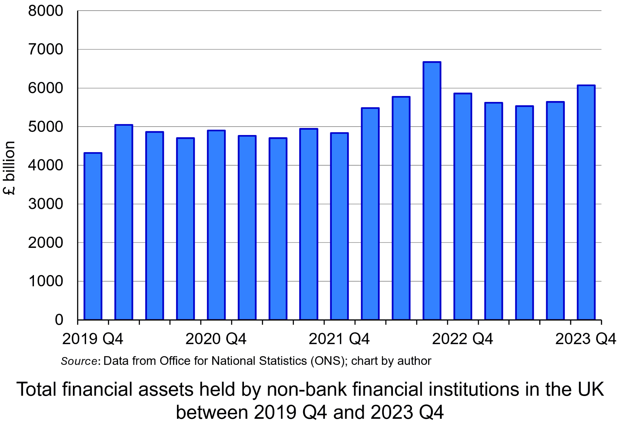 Data from the Bank of England show that the percentage of total assets held by NBFIs rose from 41% in 2007 to 49% in 2020. The chart illustrates the total financial assets held by non-bank financial institutions in the UK between 2019 Q4 and 2023 Q3 (click here for a PowerPoint). The amount held has growth by approximately a third in that time, from £4321bn to £6069bn, peaking at £6670bn in 2022 Q3.
The lack of regulatory oversight stems from the nature of the activities in the shadow banking sector. While NBFIs conduct maturity transformation, provide liquidity and help manage risk, unlike banks, they do not accept deposits and are not part of the payments system involving the general public.
Consequently, the consensus among regulators has been that their activities do not pose the same systemic risks as banking of the breakdown of the payments mechanism and associated collapse in business and consumer confidence. Therefore, NBFIs are not subject to conventional regulation and supervision involving liquidity and capital requirements.
However, as the scale of borrowing and lending running through the sector has grown, this argument has become less difficult to justify. There is a concern that ‘regulatory arbitrage’ is happening and that the systemic risks associated with shadow banking are being underestimated.
The familiar risks of shadow banking
 The systemic consequences of liquidity and solvency problems in the shadow banking sector may not seem obvious. Much of their activities are arcane and technical. However, there are plenty of examples of instances where the problems of hedge funds or pension funds have caused systemic issues.
While the consequences are not the same as those involving banks, in that the payments mechanism is not directly affected, the risks are. Just like banks, these institutions are exposed to liquidity risks, credit default risks and counterparty risks. The concern is that they do not have the same levels of liquidity or capital buffers as banks to insulate them from the consequences of such risks. Therefore, it might not take much economic stress for one or more of these institutions to fail and, given the increasing significance and interconnectedness of these activities, impose significant costs on the rest of the financial system.
It was for this reason that the Bank of England conducted its first system-wide exploratory scenario to analyse the impact of economic and market stress on these institutions and assess the nature and extent of systemic risks which resulted. Fifty City of London institutions modelled how a period of intense stress would ripple through the non-bank sector.
The scenario involved rising geopolitical tensions which caused a sharp rise in risk aversion and a demand for higher expected rates of return as compensation. This produced sharp rises in both sovereign and corporate bond yields and matching sharp declines in asset prices (remember bond yield and prices have a negative relationship).
The scenario found that the position and behaviour of NBFIs amplified the shock. These institutions invest significantly in marketable financial securities and their liquidity and solvency are susceptible to such falling prices.
The sharp decline in asset prices triggered margin calls – payments to cover open loss positions in financial securities. In response to these demands, while some NBFIs’ internal risk and leverage measures were breached, others illustrated greater risk-aversion and took precautionary action. These institutions acted to deleverage, derisk and recapitalise. Given the interconnectedness of financial markets, the individual actions of institutions rippled across financial markets, causing problems in other segments.
The significant decline in asset prices led insurance companies and pension funds to seek to improve their liquidity and solvency position by liquidating positions in money market funds and hedge funds. This, in turn, required these funds to seek liquidity. Such institutions tend to rely a lot on the repo market (involving short-term sale and repurchase credit agreements) to provide liquidity to investors. This avoids them having to sell assets. This practice has echoes of the banking sectors use of the short-term wholesale markets in the run-up to the 2008 financial crisis.
 However, the SWES found that while banks were willing to take on some of the risk, their own concerns about liquidity and counterparty credit risk meant they did not offer sufficient short-term liquidity through the repo markets. If such funding dried up because of a higher risk perception, it could compromise the hedge funds’ ability to raise funds, requiring asset sales. This would amplify the shock to financial markets, driving prices of financial securities even lower.
The scenario concluded that the resulting heavy selling could seize up financial markets, particularly the UK sovereign and corporate bond markets, reducing the ability of companies to finance investment. This is a different type of credit crunch from 2008, which was restricted to banks – but a credit crunch, nonetheless.
At the same time, funds may make capital losses as they sell securities in the downturn. This creates solvency problems and the potential for failure.
In the SWES the institutions were often not able to anticipate how their counterparties, investors, or markets they operate in would behave in the stressed scenario, which echoes the experience of banks in 2007 and 2008 – a significant reason for the ‘crunch’ in banking credit was uncertainty about the creditworthiness of counterparties, meaning that banks were not prepared to lend to anybody.
Conclusion
Since the 2008 financial crisis, there has been a tightening of the regulation and supervision of banks which has limited their ability to channel credit. This has produced an expansion in the shadow banking sector.
However, while the shadow banking sector has not been subject to the same regulation and supervision as banks, there are still potential systemic risks associated with its operations. There have been several examples of such risks in the shadow banking sector which have led regulators to pay more attention. These underpinned the 2024 system-wide exploratory scenario (SWES) conducted by the Bank of England.
The scenario showed the possible transmission mechanism through which problems for NBFIs can have broader consequences. The report nevertheless concluded that:
…the UK financial system was well-capitalised, maintained high levels of liquidity and that asset quality remained strong.
Therefore, the UK financial system was resilient enough to withstand problems in shadow banking.
Although the results of the exercise provide a ‘framework of future system-wide analysis which can be embedded in future market-wide surveillance,’ history indicates that risks tend to exist in obscure and arcane parts of the financial system and that these never tend to be fully appreciated until a crisis occurs. This then tends to involve significant costs for taxpayers.
Articles
- Bank of England warns of risks from non-banks in future markets crisis
Financial Times from MSN, Martin Arnold (29/11/24)
- BoE finds non-bank financial firms pose wider risks in crisis periods
Reuters, Lawrence White (2/12/24)
- Finance Firms Beyond Banks Not Ready For Crisis, BOE Warns
Bloomberg from Yahoo finance, Laura Noonan and Greg Ritchie (29/11/24)
- Shadow Banking System: Definition, Examples, and How It Works
Investopedia, Michael Bromberg (18/10/24)
- US Treasuries: the lessons from March’s market meltdown
Financial Times, Colby Smith and Robin Wigglesworth (29/7/20)
- LDI: the better mousetrap that almost broke the UK
FT Alphaville, Alexandra Scaggs and Louis Ashworth (29/9/22)
- Long-Term Capital Management
CFA Institute, Ron Rimkus (18/4/16)
- Neil Woodford: the continuing fallout of a scandal
Financial Times, Owen Walker (19/3/21)
Bank of England documents and reports
Data
Questions
- Explain stress testing.
- What is shadow banking? Explain the factors driving the growth of credit in this part of the financial system.
- Compare and contrast the liquidity problems of banks with those of non-bank financial institutions (NBFIs).
- Analyse how financial crises can heighten problems of asymmetric information in financial markets.
 We continue to live through incredibly turbulent times. In the past decade or so we have experienced a global financial crisis, a global health emergency, seen the UK’s departure from the European Union, and witnessed increasing levels of geopolitical tension and conflict. Add to this the effects from the climate emergency and it easy to see why the issue of economic uncertainty is so important when thinking about a country’s economic prospects.
In this blog we consider how we can capture this uncertainty through a World Uncertainty Index and the ways by which economic uncertainty impacts on the macroeconomic environment.
World Uncertainty Index
Hites Ahir, Nicholas Bloom and Davide Furceri have constructed a measure of uncertainty known as the World Uncertainty Index (WUI). This tracks uncertainty around the world using the process of ‘text mining’ the country reports produced by the Economist Intelligence Unit. The words searched for are ‘uncertain’, ‘uncertainty’ and ‘uncertainties’ and a tally is recorded based on the number of times they occur per 1000 words of text. To produce the index this figure is then multiplied up by 100 000. A higher number therefore indicates a greater level of uncertainty. For more information on the construction of the index see the 2022 article by Ahir, Bloom and Furceri linked below.
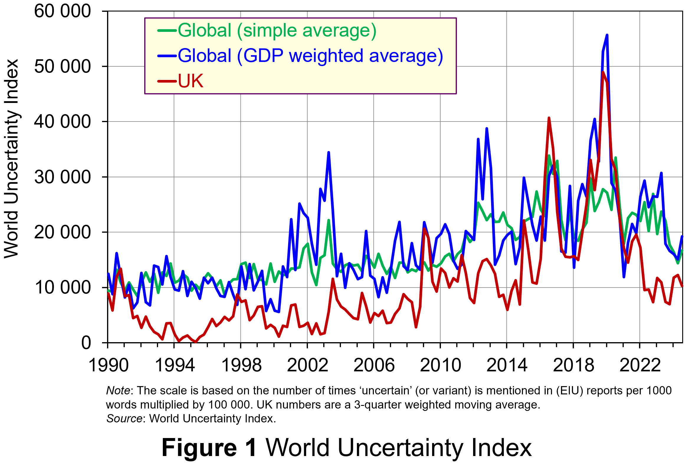 Figure 1 (click here for a PowerPoint) shows the WUI both globally and in the UK quarterly since 1991. The global index covers 143 countries and is presented as both a simple average and a GDP weighted average. The UK WUI is also shown. This is a three-quarter weighted average, the authors’ preferred measure for individual countries, where increasing weights of 0.1, 0.3 and 0.6 are used for the three most recent quarters.
From Figure 1 we can see how the level of uncertainty has been particularly volatile over the past decade or more. Events such as the sovereign debt crisis in parts of Europe in the early 2010s, the Brexit referendum in 2016, the COVID-pandemic in 2020–21 and the invasion of Ukraine in 2022 all played their part in affecting uncertainty domestically and internationally.
Uncertainty, risk-aversion and aggregate demand
Now the question turns to how uncertainty affects economies. One way of addressing this is to think about ways in which uncertainty affects the choices that people and businesses make. In doing so, we could think about the impact of uncertainty on components of aggregate demand, such as household consumption and investment, or capital expenditures by firms.
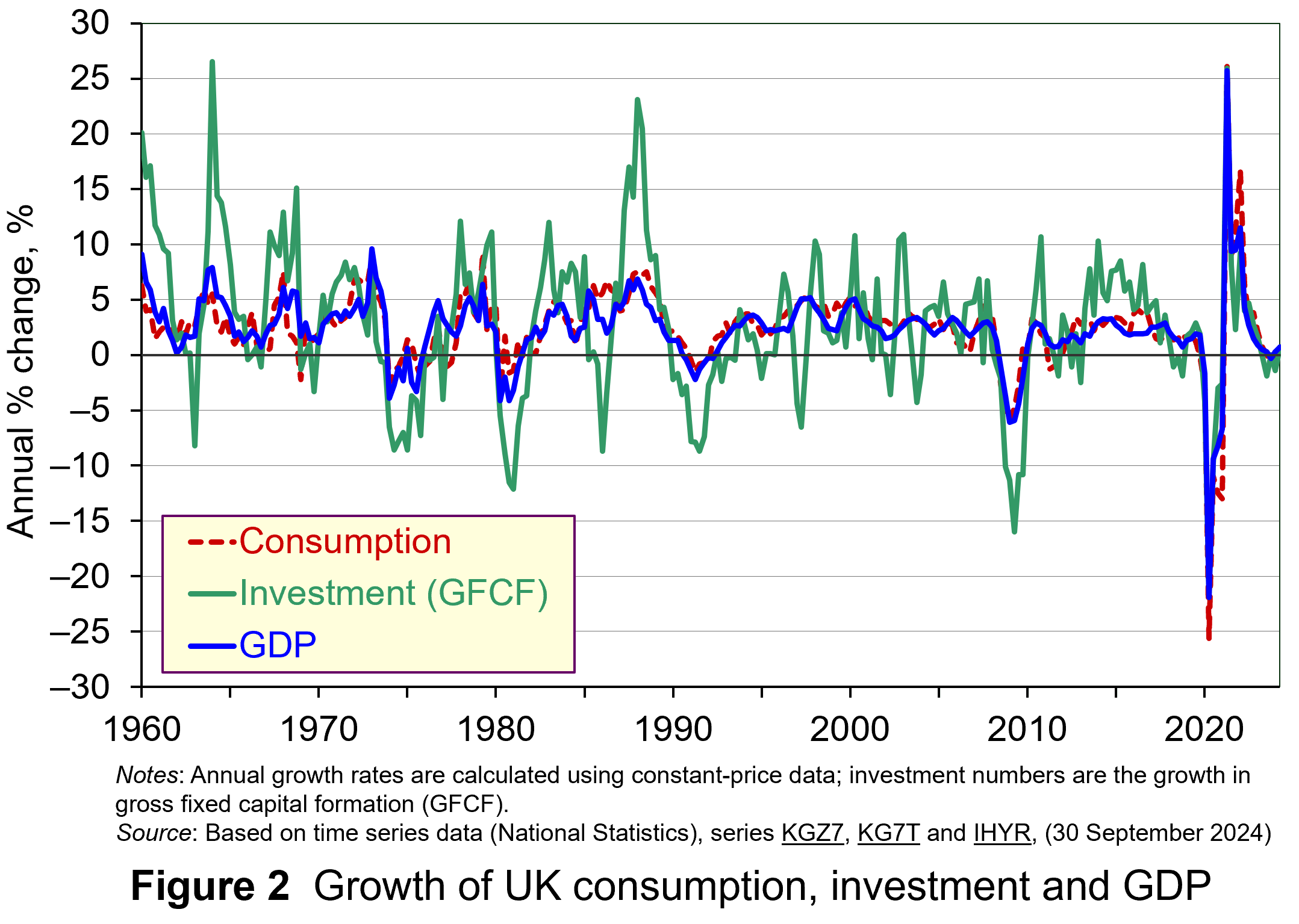 As Figure 2 shows (click here for a PowerPoint), investment is particularly volatile, and much more so than household spending. Some of this can be attributed to the ‘lumpiness’ of investment decisions since these expenditures tend to be characterised by indivisibility and irreversibility. This means that they are often relatively costly to finance and are ‘all or nothing’ decisions. In the context of uncertainty, it can make sense therefore for firms to wait for news that makes the future clearer. In this sense, we can think of uncertainty rather like a fog that firms are peering through. The thicker the fog, the more uncertain the future and the more cautious firms are likely to be.
The greater caution that many firms are likely to adopt in more uncertain times is consistent with the property of risk-aversion that we often attribute to a range of economic agents. When applied to household spending decisions, risk-aversion is often used to explain why households are willing to hold a buffer stock of savings to self-insure against unforeseen events and their future financial outcomes being worse than expected. Hence, in more uncertain times households are likely to want to increase this buffer further.
 The theory of buffer-stock saving was popularised by Christopher Carroll in 1992 (see link below). It implies that in the presence of uncertainty, people are prepared to consume less today in order to increase levels of saving, pay off existing debts, or borrow less relative to that in the absence of uncertainty. The extent of the buffer of financial wealth that people want to hold will depend on their own appetite for risk, the level of uncertainty, and the moderating effect from their own impatience and, hence, present bias for consuming today.
Risk aversion is consistent with the property of diminishing marginal utility of income or consumption. In other words, as people’s total spending volumes increase, their levels of utility or satisfaction increase but at an increasingly slower rate. It is this which explains why individuals are willing to engage with the financial system to reallocate their expected life-time earnings and have a smoother consumption profile than would otherwise be the case from their fluctuating incomes.
Yet diminishing marginal utility not only explains consumption smoothing, but also why people are willing to engage with the financial system to have financial buffers as self-insurance. It explains why people save more or borrow less today than suggested by our base-line consumption smoothing model. It is the result of people’s greater dislike (and loss of utility) from their financial affairs being worse than expected than their like (and additional utility) from them being better than expected. This tendency is only likely to increase the more uncertain times are. The result is that uncertainty tends to lower household consumption with perhaps ‘big-ticket items’, such as cars, furniture, and expensive electronic goods, being particularly sensitive to uncertainty.
Uncertainty and confidence
Uncertainty does not just affect risk; it also affects confidence. Risk and confidence are often considered together, not least because their effects in generating and transmitting shocks can be difficult to disentangle.
We can think of confidence as capturing our mood or sentiment, particularly with respect to future economic developments. Figure 3 plots the Uncertainty Index for the UK alongside the OECD’s composite consumer and business confidence indicators. Values above 100 for the confidence indicators indicate greater confidence about the future economic situation and near-term business environment, while values below 100 indicate pessimism towards the future economic and business environments.
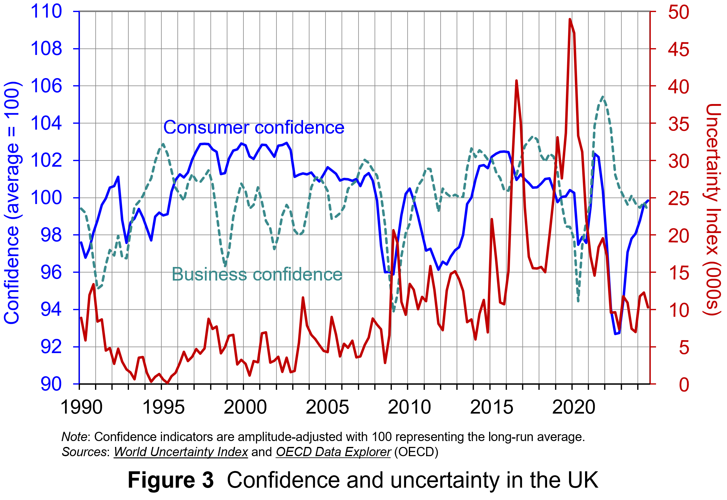 Figure 3 suggests that the relationship between confidence and uncertainty is rather more complex than perhaps is generally understood (click here for a PowerPoint). Haddow, Hare, Hooley and Shakir (see link below) argue that the evidence tends to point to changes in uncertainty affecting confidence, but with less evidence that changes in confidence affect uncertainty.
To illustrate this, consider the global financial crisis of the late 2000s. The argument can be made that the heightened uncertainty about future prospects for households and businesses helped to erode their confidence in the future. The result was that people and businesses revised down their expectations of the future (pessimism). However, although people were more pessimistic about the future, this was more likely to have been the result of uncertainty rather than the cause of further uncertainty.
Conclusion
For economists and policymakers alike, indicators of uncertainty, such as the Ahir, Bloom and Furceri World Uncertainty Index, are invaluable tools in understanding and forecasting behaviour and the likely economic outcomes that follow. Some uncertainty is inevitable, but the persistence of greater uncertainty since the global financial crisis of the late 2000s compares quite starkly with the relatively lower and more stable levels of uncertainty seen from the mid-1990s up to the crisis. Hence the recent frequency and size of changes in uncertainty show how important it to understand how uncertainty effects transmit through economies.
Academic papers
- The World Uncertainty Index
National Bureau of Economic Research, Working Paper 29763, Hites Ahir, Nicholas Bloom and Davide Furceri (February 2022)
- The Buffer-Stock Theory of Saving: Some Macroeconomic Evidence
Brookings Papers on Economic Activity, Christopher D Carroll (Vol 2, 1992)
- Macroeconomic uncertainty: what is it, how can we measure it and why does it matter?
Bank of England Quarterly Bulletin, 2013 Q2, Abigail Haddow, Chris Hare, John Hooley and Tamarah Shakir (13/6/13)
Articles
Data
Questions
- (a) Explain what is meant by the concept of diminishing marginal utility of consumption.
(b) Explain how this concept helps us to understand both consumption smoothing and the motivation to engage in buffer-stock saving.
- Explain the distinction between confidence and uncertainty when analysing macroeconomic shocks.
- Discuss which types of expenditures you think are likely to be most susceptible to uncertainty shocks.
- Discuss how economic uncertainty might affect productivity and the growth of potential output.
- How might the interconnectedness of economies affect the transmission of uncertainty effects through economies?
 In recent months there has been growing uncertainty across the global economy as to whether the US economy was going to experience a ‘hard’ or ‘soft landing’ in the current business cycle – the repeated sequences of expansion and contraction in economic activity over time. Announcements of macroeconomic indicators have been keenly anticipated for signals about how quickly the US economy is slowing.
Such heightened uncertainty is a common feature of late-cycle slowing economies, but uncertainty now has been exacerbated because it has been a while since developed economies have experienced a business cycle like the current one. The 21st century has been characterised by low inflation, low interest rates and recessions caused by various types of crises – a stock market crisis (2001), a banking crisis (2008) and a global pandemic (2020). In contrast, the current cycle is a throwback to the 20th century. The high inflation and the ensuing increases in interest rates have produced a business cycle which echoes the 1970s. Therefore, few investors have experience of such economic conditions.
The focus for investors during this stage of the cycle is when the slowing economy will reach the minimum. They will also be concerned with the depth of the slowdown: will there still be some growth in income, albeit low; or will the trough be severe enough to produce a recession, and, if so, how deep? Given uncertainty around the length and magnitude of business cycles, this leads to greater risk aversion among investors. This affects reactions to announcements of leading and lagging macroeconomic indicators.
This blog examines what sort of economic conditions we should expect in a late-cycle economy. It analyses the impact this has had on investor behaviour and the ensuing dynamics observed in financial markets in the USA.
The Business Cycle
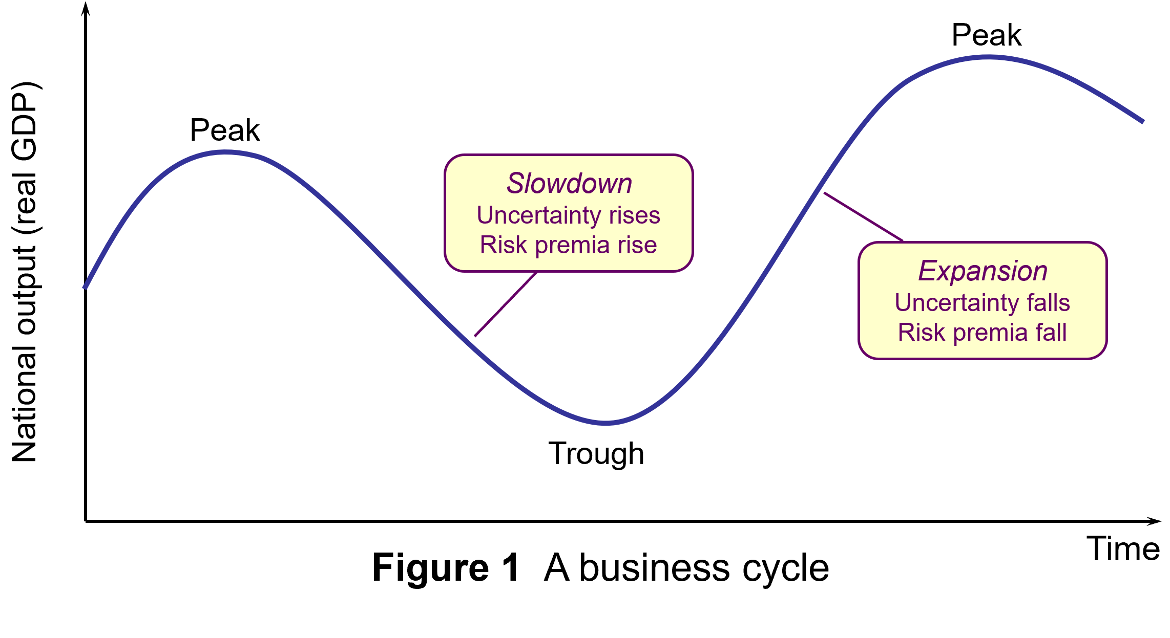
The business cycle refers to repeated sequences of expansion and contraction (or slowdown) in economic activity over time. Figure 1 illustrates a typical cycle. Typically, these sequences include four main stages. In each one there are different effects on consumer and business confidence:
- Expansion: During this stage, the economy experiences growth in GDP, with incomes and consumption spending rising. Business and consumer confidence are high. Unemployment is falling.
- Peak: This is the point at which the economy reaches its maximum output, but growth has ceased (or slowed). At this stage, inflationary pressures peak as the economy presses against potential output. This tends to result in tighter monetary policy (higher interest rates).
- Slowdown: The higher interest rates raise the cost of borrowing and reduce consumption and investment spending. Consumption and incomes both slow or fall. (Figure 1 illustrates the severe case of falling GDP (negative growth) in this stage.) Unemployment starts rising.
- Trough: This is the lowest point of the cycle, where economic activity bottoms out and the economy begins to recover. This can be associated with slow but still rising national income (a soft landing) or national income that has fallen (a hard landing, as shown in Figure 1).
While business cycles are common enough to enable such characterisation of their temporal pattern, their length and magnitude are variable and this produces great uncertainty, particularly when cycles approach peaks and troughs.
 As an economy’s cycle approaches a trough, such as US economy’s over the past few months, uncertainty is exacerbated. The high interest rates used to tackle inflation will have increased borrowing costs for businesses and consumers. Access to credit may have become more restricted. Profit margins are reduced, especially for industrial sectors sensitive to the business cycle, reducing expected cash flows.
The combination of these factors can increase the risk of a recession, producing greater volatility in financial markets. This manifests itself in increased risk aversion among investors.
Utility theory suggests that, in general, investors will exhibit loss aversion. This means that they do not like bearing risk, fearing that the return from an investment may be less than expected. In such circumstances, investors need to be compensated for bearing risk. This is normally expressed in terms of expected financial return. To bear more risk, investors require higher levels of return as compensation.
As perceptions of risk change through the business cycle, so this will change the return investors will require from the financial instruments they hold. Perceived higher risk raises the return investors will require as compensation. Conversely, lower perceived risk decreases the return investors expect as compensation.
Investors’ expected rate of return is manifested in the discount rate that they use to value the anticipated cash flows from financial instruments in discounted cash flow (DCF) analysis. Equation 1 is the algebraic expression of the present-value discounted series of cash flows for financial instruments:

Where:
V = present value
C = anticipated cash flows in each of time periods 1, 2, 3, etc.
r = expected rate of return
For fixed-income debt securities, the cash flow is constant, while for equity securities (shares), expectations regarding cash flows can change.
Slowing economies and risk aversion
 In a slowing economy, with great uncertainty about the scale and timing of the bottom of the cycle, investors become more risk averse about the prospects of firms. This this leads to higher risk premia for financial instruments sensitive to a slowdown in economic activity.
This translates into a higher expected return and higher discount rate used in the valuation of these instruments (r in equation 1). This produces decreases in perceived value, decreased demand and decreased prices for these financial instruments. This can be observed in the market dynamics for these instruments.
First, there may be a ‘flight to safety’. Investors attach a higher risk premium to risker financial instruments, such as equities, and seek a ‘safe-haven’ for their wealth. Therefore, we should observe a reorientation from more risky to less risky assets. Demand for equities falls, while demand for safer assets, such as government bonds and gold, rises.
There is some evidence for this behaviour as uncertainty about the US economic outlook has increased. Gold, long seen as a hedge against market decline, is at record highs. US Government bond prices have risen too.
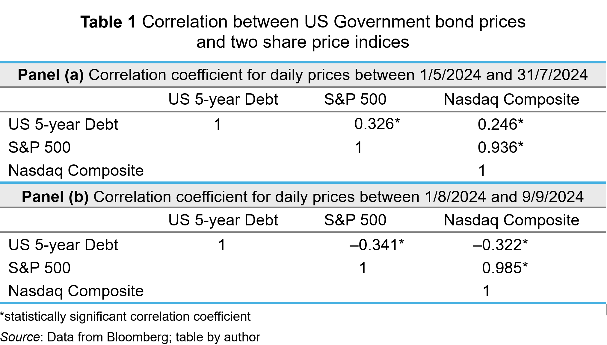
To analyse whether this may be a flight to safety, I analysed the correlation between the daily US government bond price (5-year Treasury Bill) and share prices represented by the two more significant stock market indices in the USA: the S&P 500 and the Nasdaq Composite. I did this for two different time periods. Table 1 shows the results. Panel (a) shows the correlation coefficients for the period between 1 May 2024 and 31 July 2024; Panel (b) shows the correlation coefficients for the period between 1 August 2024 and 9 September 2024.

In the period between May and July 2024, the 5-year Treasury Bill and share price indices had significantly positive correlations. When share prices rose, the Treasury Bill’s price rose; when share prices fell, the bill’s price fell. During that period, expectations about falling interest rates dominated valuations and that effected the valuations of all financial instruments in the same way – lower expected interest rates reduce the opportunity cost of holding instruments and reduces the expected rates of return. Hence, the discount rate applied to cash flows is reduced, and present value rises. The opposite happens when macroeconomic indicators suggest that interest rates will stay high (ceteris paribus).
As the summer proceeded, worries about a ‘hard landing’ began to concern investors. A weak jobs report in early August particularly exercised markets, producing a ‘flight to safety’. Greater risk aversion among investors meant that they expect a higher return from equities. This reduced perceived value, reducing demand and price (ceteris paribus). To insulate themselves from higher risk, investors bought safer assets, like government bonds, thereby pushing up their prices. This behaviour was consistent with the significant negative correlation observed between US government debt prices and the S&P 500 and Nasdaq indices in Panel (b).
Another signal of increased risk aversion among investors is ‘sector rotation’ in their equity portfolios. Increased risk aversion among investors will lead them to divest from ‘cyclical’ companies. Such companies are in industrial sectors which are more sensitive to the changing economic conditions across the business cycle – consumer discretionary and communication services sectors, for example. To reduce their exposure to risk, investors will switch to ‘defensive’ sectors – those less sensitive to the business cycle. Examples include consumer staples and utility sectors.
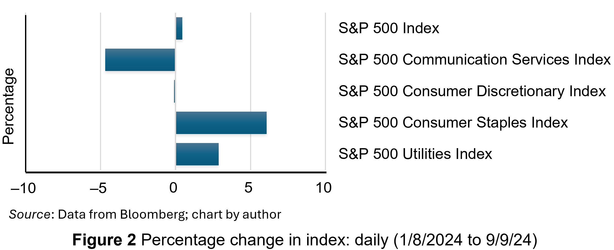
Cyclical sectors will suffer a greater adverse impact on their cash flows and risk in a slowing economy. Consequently, investors expect higher return as compensation. This reduces the value of those shares. Demand for them falls, depressing their price. In contrast, defensive sectors will be valued more. They will see an increase in demand and price. This sector rotation seems to have happened in August (2024). Figure 2 shows the percentage change between 1 August and 9 September 2024 in the S&P 500 index and four sector indices, comprising companies from the communication services, consumer discretionary, consumer staples and utilities sectors.

Overall, the S&P 500 index was slightly higher, as shown by the first bar in the chart. However, while the cyclical sectors experienced decreases in their share prices, particularly communication services, the defensive companies experienced large price increases – nearly 3% for utilities and over 6% for consumer staples.
Conclusion
Economies experience repeated sequences of expansion and contraction in economic activity over time. At the moment, the US economy is approaching the end of its current slowing phase. Increased uncertainty is a common feature of late-cycle economies and this manifests itself in heightened risk aversion among investors. This produces certain dynamics which have been observable in US debt and equity markets. This includes a ‘flight to safety’, with investors divesting risky financial instruments in favour of safer ones, such as US government debt securities and gold. Also, investors have been reorientating their equity portfolios away from cyclicals and towards defensive securities.
Articles
- America’s recession signals are flashing red. Don’t believe them
The Economist (22/8/24)
- The most well-known recession indicator stopped flashing red, but now another one is going off
CNN, Elisabeth Buchwald (13/9/24)
- World’s largest economy will still achieve soft landing despite rising unemployment, most analysts believe
Financial Times, Claire Jones, Delphine Strauss and Martha Muir (6/8/24)
- We’re officially on slowdown watch
Financial Times, Robert Armstrong and Aiden Reiter (30/8/24)
- Anatomy of a rout
Financial Times, Robert Armstrong and Aiden Reiter (6/8/24)
- Reasons why investors need to prepare for a US recession
Financial Times, Peter Berezin (5/9/24)
- Business Cycle: What It Is, How to Measure It, and Its 4 Phases
Investopedia, Lakshman Achuthan (6/6/24)
- Risk Averse: What It Means, Investment Choices, and Strategies
Investopedia, James Chen (5/8/24)
Data
Questions
- What is risk aversion? Sketch an indifference curve for a risk-averse investor, treating expected return and risk as two-characteristics of a financial instrument.
- Show what happens to the slope of the indifference curve if the investor becomes more risk averse.
- Using demand and supply analysis, illustrate and explain the impact of a flight to safety on the market for (i) company shares and (ii) US government Treasury Bills.
- Use economic theory to explain why the consumer discretionary sector may be more sensitive than the consumer staples sector to varying incomes across the economic cycle.
- Research the point of the economic cycle that the US economy has reached as you read this blog. What is the relationship between bond and equity prices? Which sectors have performed best in the stock market?
When anyone buys assets – shares, a house, a car or whatever – one important consideration is their likely future value. But the future is uncertain. Your decision to buy, therefore, depends not just on the direct return of the asset (the rate of interest or the pleasure from using the asset) but also on your predictions about the future value of the asset and your attitudes to risk. But with the future of markets so uncertain, or at least the timing of market movements, what’s the best thing to do? The article below considers some of the issues.
The irrelevant future Investors Chronicle (6/4/09)
Questions
- Distinguish between ‘risk’ and ‘uncertainty’.
- What is meant by a ‘bear’ in the context of investing in shares? Explain why ‘intelligent bears’ would ‘leave some money in the market’.
- Faced with uncertainty, why might sticking to a simple ‘do nothing’ rule be the best policy?
- If capital markets were efficient in the strongest sense, where everyone has perfect information about the future, would people be able to make large returns on investing in shares and other assets?
 On the 29 November, the Bank of England published the results of its latest stress test of the UK financial system. Annual stress testing was introduced in the wake of the 2008 financial crisis. It models the ability of the financial system to withstand severe macroeconomic and financial market conditions. Typically, the focus has been on testing the resilience of the banking system.
 Stress testing was introduced by the Bank of England after the financial crisis to assess the ability of the financial system to withstand severe economic and market scenarios.
 Shadow banking refers to borrowing and lending which occurs outside the banking sector. Traditionally banking involves taking deposits and using these to finance lending.
 Data from the Bank of England show that the percentage of total assets held by NBFIs rose from 41% in 2007 to 49% in 2020. The chart illustrates the total financial assets held by non-bank financial institutions in the UK between 2019 Q4 and 2023 Q3 (click here for a PowerPoint). The amount held has growth by approximately a third in that time, from £4321bn to £6069bn, peaking at £6670bn in 2022 Q3.
 The systemic consequences of liquidity and solvency problems in the shadow banking sector may not seem obvious. Much of their activities are arcane and technical. However, there are plenty of examples of instances where the problems of hedge funds or pension funds have caused systemic issues.
  However, the SWES found that while banks were willing to take on some of the risk, their own concerns about liquidity and counterparty credit risk meant they did not offer sufficient short-term liquidity through the repo markets. If such funding dried up because of a higher risk perception, it could compromise the hedge funds’ ability to raise funds, requiring asset sales. This would amplify the shock to financial markets, driving prices of financial securities even lower.
 We continue to live through incredibly turbulent times. In the past decade or so we have experienced a global financial crisis, a global health emergency, seen the UK’s departure from the European Union, and witnessed increasing levels of geopolitical tension and conflict. Add to this the effects from the climate emergency and it easy to see why the issue of economic uncertainty is so important when thinking about a country’s economic prospects.
 Figure 1 (click
  As Figure 2 shows (click
  The theory of buffer-stock saving was popularised by Christopher Carroll in 1992 (see link below). It implies that in the presence of uncertainty, people are prepared to consume less today in order to increase levels of saving, pay off existing debts, or borrow less relative to that in the absence of uncertainty. The extent of the buffer of financial wealth that people want to hold will depend on their own appetite for risk, the level of uncertainty, and the moderating effect from their own impatience and, hence, present bias for consuming today.
 Figure 3 suggests that the relationship between confidence and uncertainty is rather more complex than perhaps is generally understood (click
  In recent months there has been growing uncertainty across the global economy as to whether the US economy was going to experience a ‘hard’ or ‘soft landing’ in the current business cycle – the repeated sequences of expansion and contraction in economic activity over time. Announcements of macroeconomic indicators have been keenly anticipated for signals about how quickly the US economy is slowing.
 As an economy’s cycle approaches a trough, such as US economy’s over the past few months, uncertainty is exacerbated. The high interest rates used to tackle inflation will have increased borrowing costs for businesses and consumers. Access to credit may have become more restricted. Profit margins are reduced, especially for industrial sectors sensitive to the business cycle, reducing expected cash flows.
 In a slowing economy, with great uncertainty about the scale and timing of the bottom of the cycle, investors become more risk averse about the prospects of firms. This this leads to higher risk premia for financial instruments sensitive to a slowdown in economic activity.