 The gold market has become one of the most talked-about commodity markets in 2025, with prices reaching record highs. This is largely due to increased demand from investors, who see gold as a ‘safe haven’ during times of economic and political uncertainty. Central banks are also buying more gold as a way to reduce their reliance on currencies like the US dollar. With many analysts predicting prices could reach over $4000 per ounce in the next year, the gold market is showcasing how supply and demand, confidence, and global events can all influence a commodity market.
The commodities market is where basic agricultural products, raw materials and metals, such as gold, are bought and sold, often in large quantities and across global exchanges. Commodities are typically traded either in their physical form (like gold bars) at current market prices (spot prices) or through financial contracts, where investors buy or sell in futures markets. These are where a price is agreed today to buy or sell on a specific future date.
As with other commodities, the price of gold is determined by supply and demand. Demand for gold typically rises during times of economic uncertainty as investors want a safer store of value. This results in an increase in its price. Supply and demand, and hence price, also respond to other factors, including interest rates, currency movements, economic growth and growth prospects, and geopolitical events.
Record high prices
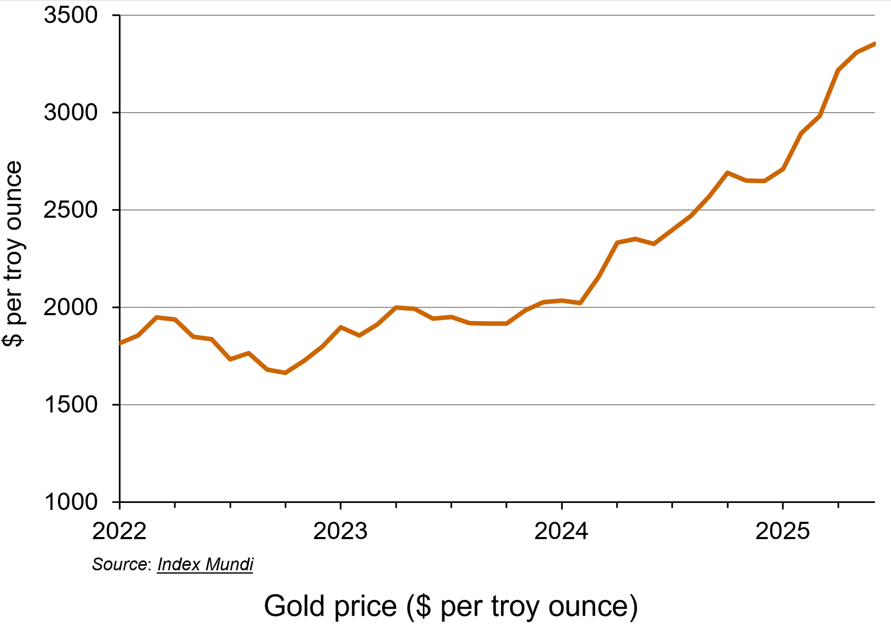 This year, the gold market has seen a remarkable rally, with the price of gold hitting a record high. Demand for the precious metal has resulted in spot prices surging over 35% to date (see the chart: click here for a PowerPoint). Rising prices earlier this year have been attributed to the US President, Donald Trump, announcing wide-ranging tariffs which have upset global trade. On 2 September, the spot gold price hit $3508.50 per ounce, continuing its upwards trend.
The price has also been lifted by expectations that the Federal Reserve (the US central bank) will cut its key interest rate, making gold an even more attractive prospect for investors. If the Federal Reserve cuts interest rates, the price of gold usually increases. This is because gold does not pay any interest or yield, so when interest rates are high, investors can earn better returns from alternatives, such as savings accounts or bonds. However, when interest rates fall, those returns become less attractive, making gold relatively more appealing.
Lower interest rates also tend to weaken the US dollar, which makes gold cheaper for foreign buyers, increasing global demand. Since gold is priced in dollars, a weaker dollar usually leads to higher gold prices.
Additionally, interest rate cuts are often a response to economic problems or uncertainty. As gold is viewed as a safer asset for investors during times of economic uncertainty, investors will typically increase their demand.
Unlike the market for currencies or shares, gold doesn’t rely on the performance of a government or company. This makes it attractive when people are worried about things like inflation, recession, war or stock market crashes. Gold is thus seen as a ‘safe haven’.
Gold and the Federal Reserve
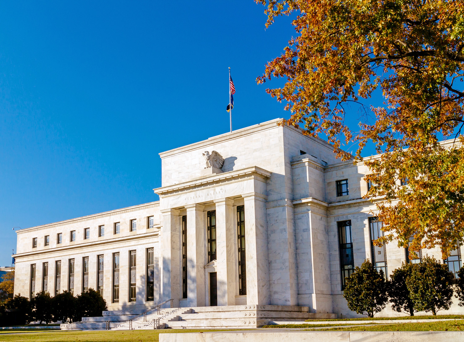 The rise in the price of gold by more than a third this year can be linked to the US election last year, according to the director of research at BullionVault (see the BBC article below). Attitudes of the Trump administration towards the Federal Reserve have created concerns among investors. Fears that the US administration could erode the independence of the world’s most important central bank have fuelled the latest flows into the metal, which is traditionally viewed as a hedge against inflation.
According to the BBC article, Derren Nathan from Hargreaves Lansdown claims that it is Trump’s ‘attempts to undermine the independence of the Federal Reserve Bank’ that were ‘driving renewed interest in safe haven assets, including gold’. Investors are concerned that a politicised Fed would be more inclined to cut interest rates than would otherwise be the case, sending long-term inflation expectations higher.
This could lead to fears that future interest rates would then be pushed higher. This would increase the yields on longer-term government bonds by pushing down their price, as investors demand higher compensation for the increased risk of higher future interest rates reducing the value of their fixed-rate investments. This would force the US Treasury to pay higher interest on new bonds, making it more expensive to service US government debt.
Expected price rises for 2026
As we saw above, it is predicted that the price of gold will rise to $4000 per ounce next year. However, if the market sees investors move away from dollar assets, such as US Treasuries, the price increases would be even higher. Daan Struyven, co-head of global commodities research at Goldman Sachs explains ‘If 1 per cent of the privately owned US Treasury market were to flow to gold, the gold price would rise to nearly $5000 per troy ounce’ (see Financial Times article below).
 If the Federal Reserve does come under political pressure, it could affect the stability of the US economy and beyond. When gold prices rise sharply, demand usually falls in countries like China and India, which are the world’s largest buyers of gold jewellery. However, in 2025, this trend has changed. Instead of reducing their gold purchases, people in these countries have started buying investment gold, such as bars and coins, showing a shift in consumer behaviour from jewellery to investment assets.
At the same time, global events are also influencing the gold market. Suki Cooper, a metals analyst at Standard Chartered, said that events like Russia’s invasion of Ukraine have added to political uncertainty, which tends to increase demand for gold as a safe-haven asset. She also highlighted how changes in international trade policies have disrupted supply chains and contributed to higher inflation, both of which have made gold more attractive to investors. Additionally, a weaker US dollar earlier in the year made gold cheaper for buyers using other currencies, which boosted global demand even further.
Conclusion
Although the gold market is expected to remain strong over the next six months, some uncertainty remains. Many analysts predict that gold prices will stay high or even increase further, especially if interest rates in the US are cut as expected. Continued global instability, is also likely to keep demand for gold as a safe haven high. At the same time, if inflation stays elevated or trade disruptions continue, more investors may turn to gold to protect their wealth.
However, if economic conditions stabilise or interest rates rise again, gold demand could fall slightly, leading to a potential dip in prices. Overall, the outlook for gold remains positive, but sensitive to changes in global economic and political events.
Articles
- Gold price hits record high as investors seek safety
BBC News, Faarea Masud (2/9/25)
- Safe-haven gold rally gains further momentum after soft US data
Reuters, Sherin Elizabeth Varghese and Ashitha Shivaprasad (3/9/25)
- Gold vaults $3,000 in rush for safety from market, political worry
Reuters, Sherin Elizabeth Varghese and Anmol Choubey (14/3/25)
 The foundation of gold’s rally to historic highs started back in 2022
CNBC, Suki Cooper (17/3/25)
- Gold could hit nearly $5,000 if Trump undermines Fed, says Goldman Sachs
Financial Times, Emily Herbert (4/9/25)
- London’s bullion market set to trial digital gold
City AM, Maisie Grice (3/8/25)
- Gold price hits record high as investors seek safe haven
The Guardian, Julia Kollewe (2/9/25)
Data
Questions
- What factors influence the price of a commodity such as gold on the global market?
- Use a demand and supply diagram to illustrate what has been happening to the gold price in recent months.
- Find out what has been happening to silver prices. Are the explanations for the price changes the same as for gold?
- Why might investors choose to buy gold during times of economic or political uncertainty?
- How will changes in interest rates affect both the demand for and the price of gold?
- What are the possible consequences of rising gold prices for countries like India and China, where there is a traditionally high demand for gold jewellery?
- How do global events impact commodity markets? Use gold as an example in your answer.
 On 25 October 2024, Moody’s, one of the major credit ratings agencies, announced that it was downgrading France’s economic outlook to negative. This was its first downgrading of France since 2012. It followed a similar revision by Fitch’s, another ratings agency, on 11 October.
While Fitch’s announcement did not have a significant impact on the yields of French government bonds, expectations around Moody’s did. In the week preceding the announcement, the net increases in the yield on generic 10-year government debt was approximately 9 basis points (0.09 percentage points). On the day itself, the yield rose by approximately 5.6 basis points (0.056 percentage points).
The yield rose further throughout the rest of October, finishing nearly 0.25 percentage points above its level at the start of the month. However, as Figure 1 illustrates, these increases are part of a longer-term trend of rising yields for French government debt (click here for a PowerPoint).
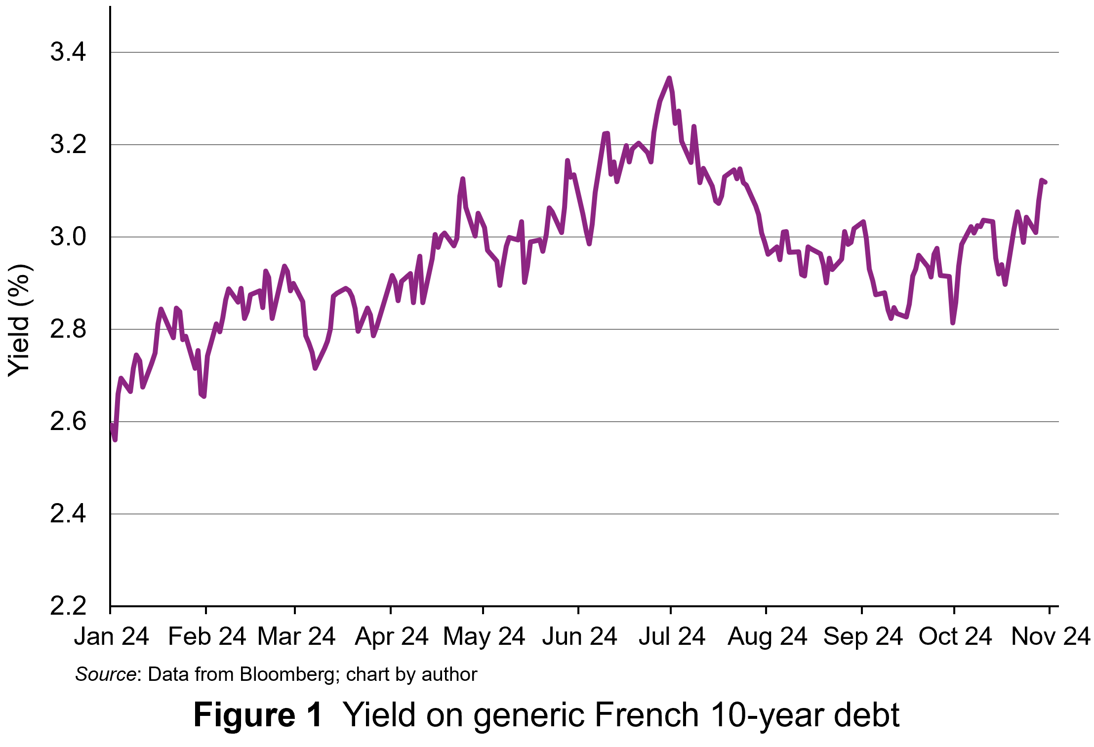 The yield on 10-year French government debt began 2024 at 2.56% and had an upward trend for the first half of the year. The yield peaked at 3.34% on 1 July. It then fell back below 3% for a while. The negative economic outlook then pushed yields back above 3% and they finished October at 3.12%, half a percentage point above the level at the start of the year. This represents a significant increase in borrowing costs for the French government.
In this blog, we will explain why the changes in France’s economic outlook translate into increases in yields for French government bonds. We will also analyse why yields have increased and examine the prospects for the markets in French government bonds.
Pricing signals of bond yields
A bond is a tradable debt instrument issued by governments to finance budget deficits – the difference between tax receipts and spending. Like any financial instruments, investment in bonds involves a commitment of funds today in anticipation of interest payments through time as compensation, with a repayment of its redemption value on the date the bond matures.
Since the cash flows associated with holding a bond occur at different points in time, discounted cash flow analysis is used to determine its value. This gives the present value of the cash flows discounted at the appropriate expected rate of return. In equilibrium this will be equal to the bond’s market price, as the following equation shows.

Where:
P = the equilibrium price of the bond
C = cash coupon payments
M = redemption value at maturity
r = yield (expected rate of return in equilibrium.
Interest payments tend to be fixed at the time a bond is issued and reflect investors’ expected rate of return, expressed as the yield in bond markets. This is determined by prevailing interest rates and perceived risk. Over time, changes in interest rates and perceptions of risk will change the expected rate of return (yield), which will, in turn, change the present value of the cash flows, and hence fundamental value.
Prices move in response to changes in fundamental value and since this happens frequently, this means that prices change a lot. For bonds, as the coupon payments (C each year and the redemption price () are fixed, the only factor that can change is the expected rate of return (yield). This is reflected in the observed yield at each price.
 If the expected rate of return rises, this increases the discount rate applied to future cash flows and reduces their present value. At the current price, the fixed coupon is not sufficient to compensate investors. So, investors sell the bonds and price falls until it reaches a point where the yield offered is equal to that required. The reverse happens if the expected rate of return falls.
The significant risk associated with bonds is credit default risk – the risk that the debt will not be repaid. The potential for credit default is a significant influence of the compensation investors require for holding debt instruments like bonds (ceteris paribus). An increase in expected credit default risk will increase the expected return (compensation). This will be reflected in a lower price and higher yield.
Normally, with the bonds issued by high-income countries, such as those in Europe and North America, the risk of default is extremely low. However, if a country’s annual deficits or accumulated debt increase to what markets consider to be unsustainable levels, the perceived risk of default may rise. Countries’ levels of risk are rated by international ratings agencies, such as Moody’s and Fitch. Investors pay a lot of attention to the information provided by such agencies.
Moody’s downgrade in its economic outlook for France from ‘stable’ to ‘negative’ indicated weak economic performance and higher credit default risk. This revision rippled through bond markets as investors adjusted their views of the country’s economic risk. The rise in yields observed is a signal that bond investors perceive higher credit default risk associated with French government debt and are demanding a higher rates of return as compensation.
Why has France’s credit default risk premium risen now?
As we have seen, credit default risk is not normally considered a significant issue for sovereign borrowers like France. Some of the issue around perceived credit default risk for the French government relate to the size of the French government’s deficit and the projections for it. Following a spike in borrowing associated with the COVID-19 pandemic in 2020, the annual government budget deficit and the overall level of debt as percentages of GDP have remained high. The annual deficit is projected to be 6% for 2024 and still 5% for 2025. The ratio of outstanding French government debt to Gross Domestic Product (GDP) ballooned to 123% in 2020 and is still expected to be 115% by the end of 2025. France has been put on notice to reduce its debt towards the Eurozone limit of 60% of GDP.
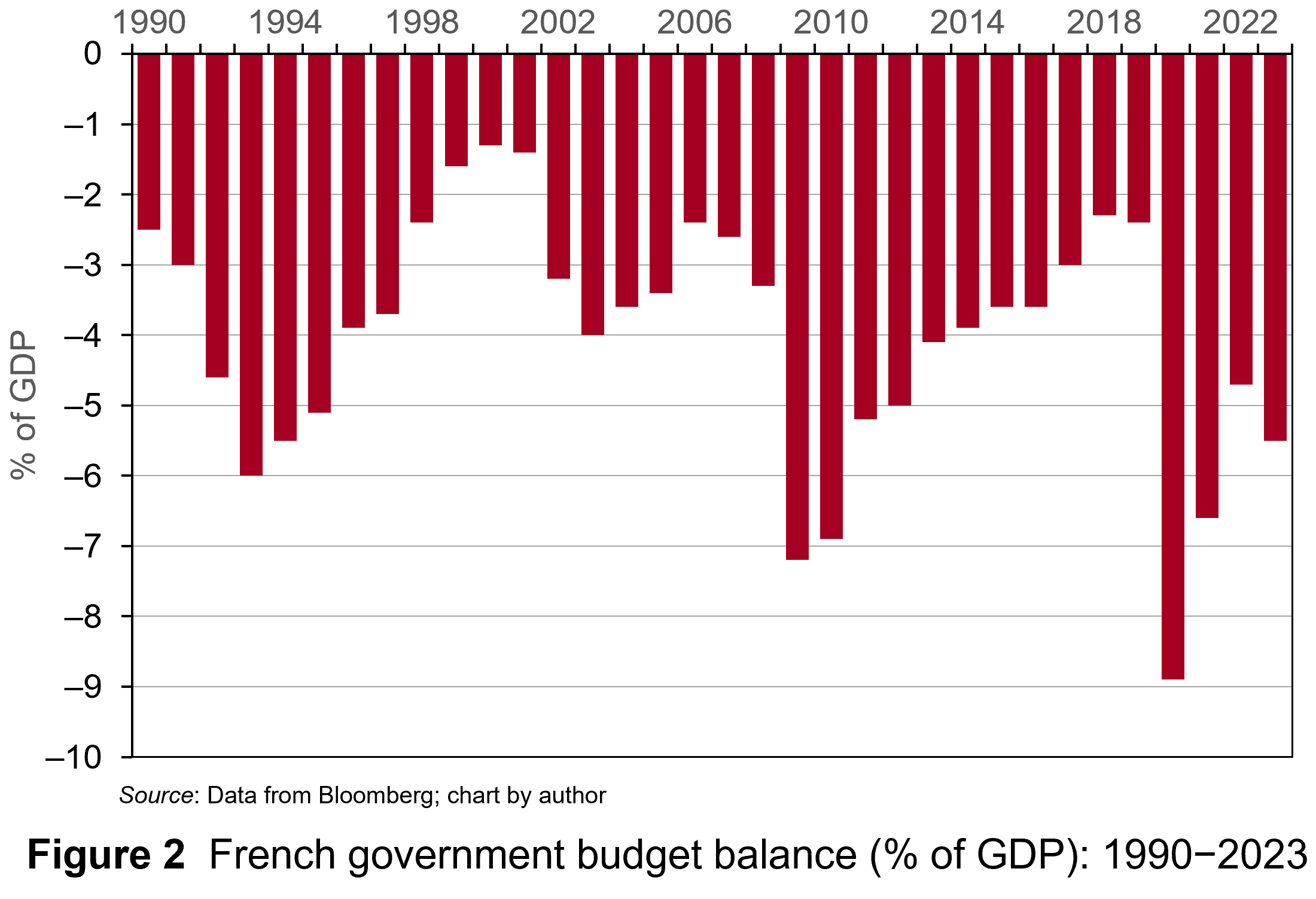 Governments in France last achieved a balanced budget in 1974. They have run deficits ever since. Figure 2 illustrates the French government budget deficits from 1990 to 2023 (click here for a PowerPoint). The figure shows that France experienced deficits in the past similar to today’s. These, however, did not tend to worry bond markets too much.
So why are investors currently worried? This stems from France’s debt mountain and from concerns that the government will not be able to deal with it. Investors are concerned that both weak growth and increasingly volatile politics will thwart efforts to reduce debt levels.
Let’s take growth. Even by contemporary European standards, France’s growth prospects are anaemic. GDP is expected to grow by just 1.1% for 2024 and 1% for 2025. Both consumer and business confidence are low. None of this suggests a growth spurt soon which will boost the tax revenues of the French government sufficiently to address the deficit.
 Further, political instability has grown due to the inconclusive parliamentary elections which Emmanuel Macron surprisingly called in July. No single political grouping has a majority and the President has appointed a Centrist Prime Minister, Michel Barnier (the former EU Brexit negotiator). His government is trying to pass a budget through the Assemblée Nationale involving a mixture of spending cuts and tax hikes which amount to savings of €60 billion ($66 billion). This is equivalent to 2% of GDP.
The parliamentary path of the budget bill is set to be torturous with both the left and right wing blocs in the Assemblée opposing most of the provisions. Debate in the Assemblée Nationale and Senate are expected to drag on into December, with the real prospect that the government may have to use presidential decree to pass the budget. Commentators argue that this will fuel further political chaos.
France looks more like Southern Europe
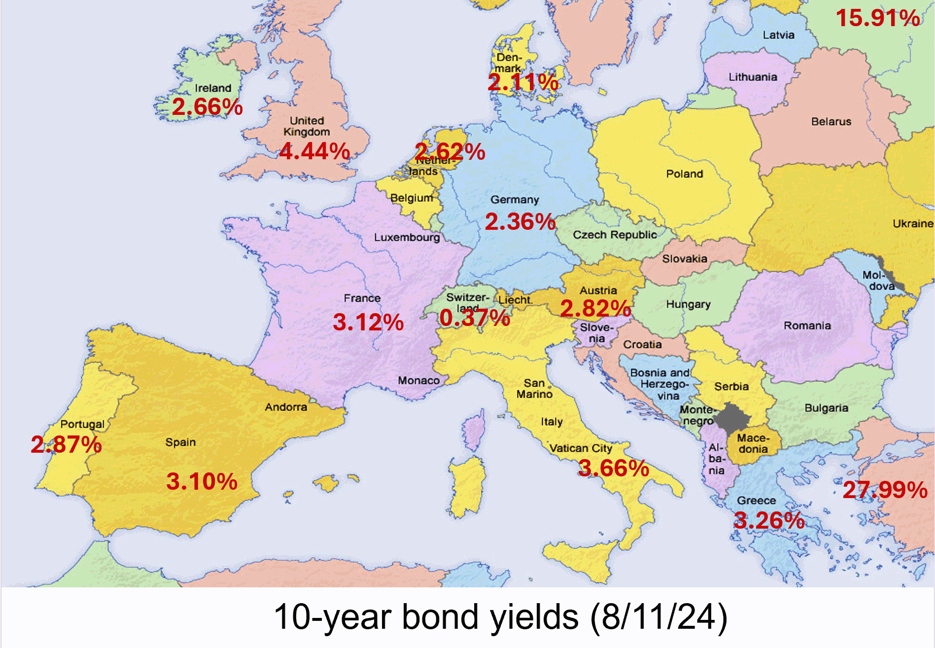 In the past, bond investors were more tolerant of France’s budget deficits. French government bonds were attractive options for investors wanting to hold euro-denominated bonds while avoiding riskier Southern European countries such as Greece, Italy, Portugal and Spain. Since France has run persistent government deficits for a long time, it offered bond investors a more liquid market than more fiscally-parsimonious Northern European neighbours, such as Germany and the Netherlands. Consequently, France’s debt instruments offered a slight risk premium on the yields for those countries.
However, that has changed. France’s credit default risk premium is rising to levels comparable to its Southern neighbours. On 26 September 2024, the yield on generic French government 10-year debt rose above its Spanish equivalent for the first time since 2008.
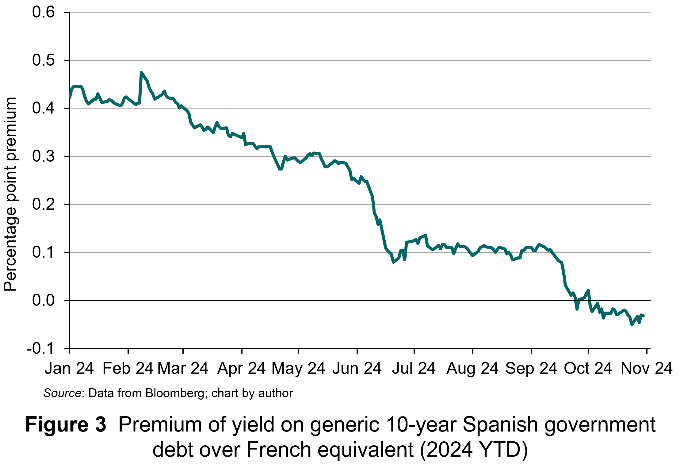 As Figure 3 illustrates, this was the culmination of a trend evident throughout 2024, with the difference in yields between the two declining steadily (click here for a PowerPoint). At the start of the year, the yield on Spanish debt offered a 40 basis points premium over the French equivalent. By October, the yield on Spanish debt was consistently below that of French debt. All of this is due to bond investors’ rising expectations about France’s credit default risk. Now, France’s borrowing costs are not only above Spain, but also closer to those of Greece and Italy than of Germany.
Strikingly, Spain’s budget deficit was 3.5% in 2023 and is expected to narrow to 2.6% by 2025. The percentage of total debt to GDP is 104% and falling. Moreover, following Spain’s inconclusive election in 2023, the caretaker government put forward budgetary plans involving fiscal tightening without the need for legislation. This avoided the political wrangling France is facing.
For France, these developments raise the prospect of yields rising further as bond investors now see alternatives to French government debt in the form of Spain’s. This country have already undertaken the painful fiscal adjustments that France seems incapable of completing.
Articles
Data
Questions
- What is credit default risk?
- Explain why higher credit default risk is associated with higher yields on France’s government debt.
- Why would low economic growth worsen the government’s budget deficit?
- Why would political instability increase credit default risk?
- What has happened to investors’ perceptions of the risk associated with French government debt relative to Spain’s?
- How has this manifested itself in the relative yields of the two countries’ government debt?
 Sustainability has become one of the most pressing issues facing society. Patterns of human production and consumption have become unsustainable. On the environmental front, climate change, land-use change, biodiversity loss and depletion of natural resource are destabilising the Earth’s eco-system.
Furthermore, data on poverty, hunger and lack of healthcare show that many people live below minimum social standards. This has led to greater emphasis being placed on sustainable development: ‘development that meets the needs of the present without compromising the ability of future generations to meet their own needs’ (The Brundtland Report, 1987: Ch.2, para. 1).
The financial system has an important role to play in channelling capital in a more sustainable way. Since current models of finance do not consider the welfare of future generations in investment decisions, sustainable finance has been developed to analyse how investment and lending decisions can manage the trade-off inherent in sustainable development: sacrificing return today to enhance the welfare of future generations.
However, some commentators argue that such trade-offs are not required. They suggest that investors can ‘do well by doing good’. In this blog, I will use ‘green’ bonds (debt instruments which finance projects or activities with positive environmental and social impacts) to explain the economics underpinning sustainable finance and show that doing good has a price that sustainable investors need to be prepared to pay.
I will analyse why investors might not be doing so and point to changes which may be required to ensure financial markets channel capital in a way consistent with sustainable development.
The growth of sustainable finance
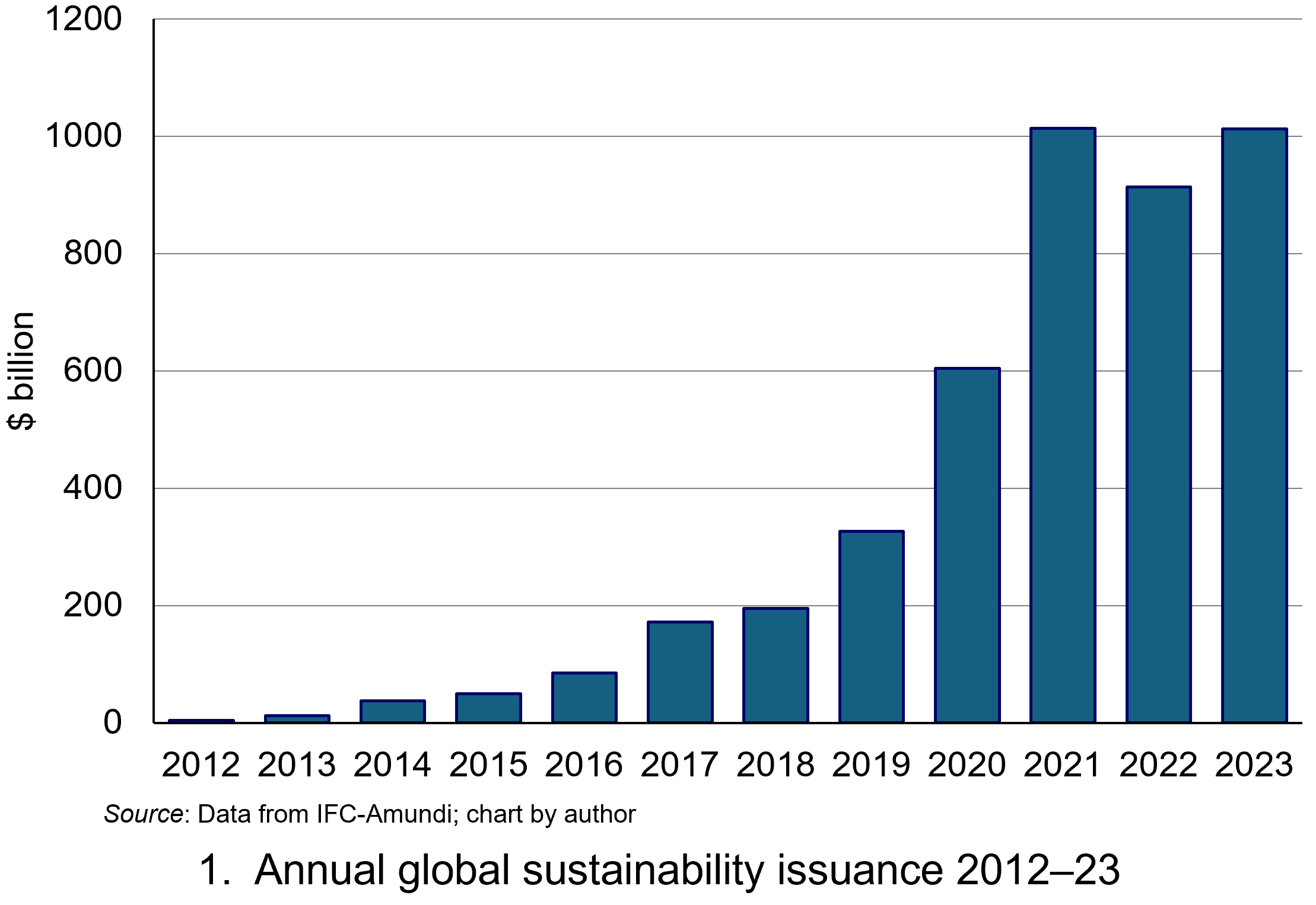 Sustainable finance has grown rapidly over the past decade as concerns about climate change have intensified. A significant element of this growth has been in global debt markets.
Figure 1 illustrates the rapid growth in the issuance of sustainability-linked debt instruments since 2012. While issuance fell in 2022 due to concerns about rising inflation and interest rates reducing the real return of fixed-income debt securities, it rebounded in 2023 and is on course for record levels in 2024. (Click here for a PowerPoint.)
Green bonds are an asset class within sustainability-linked debt. Such bonds focus on financing projects or activities with positive environmental and social impacts. They are typically classified as ‘use-of-proceeds’ or asset-linked bonds, meaning that the proceeds raised from their issuance are earmarked for green projects, such as renewable energy, clean transportation, and sustainable agriculture. Such bonds should be attractive to investors who want a financial return but also want to finance investments with a positive environmental and/or social impact.
One common complaint from commentators and investors is the ‘greenium’ – the price premium investors pay for green bonds over conventional ones. This premium reduces the borrowing costs of the issuers (the ‘counterparties’) compared to those of conventional counterparties. This produces a yield advantage for issuers of green bonds (price and yield have a negative relationship), reducing their borrowing costs compared to issuers of conventional bonds.
An analysis by Amundi in 2023 using data from Bloomberg estimated that the average difference in yield in developed markets was –2.2 basis points (–0.022 percentage points) and the average in emerging markets was –5.6 basis points (–0.056 percentage points). Commentators and investors suggest that the premium is a scarcity issue and once there are sufficient green bonds, the premium over non-sustainable bonds should disappear.
However, from an economics perspective, such interpretations of the greenium ignore some fundamentals of economic valuation and the incentives and penalties through which financial markets will help facilitate more sustainable development. Without the price premium, investors could buy sustainable debt at the same price as unsustainable debt, earn the same financial return (yield) but also achieve environmental and social benefits for future generations too. Re-read that sentence and if it sounds too good to be true, it’s because it is too good to be true.
‘There is no such thing as a free lunch’
In theory, markets are institutional arrangements where demand and supply decisions produce price signals which show where resources are used most productively. Financial markets involve the allocation of financial capital. Traditional economic models of finance ignore sustainability when appraising investment decisions around the allocation of capital. Consequently, such allocations do not tend to be consistent with sustainable development.
In contrast, economic models of sustainable finance do incorporate such impacts of investment decisions and they will be reflected in the valuation, and hence pricing, of financial instruments. Investors, responding to the pricing signals will reallocate capital in a more sustainable manner.
 Let’s trace the process. In models of sustainable finance, financial instruments such as green bonds funding investments with positive environmental impacts (such as renewable energy) should be valued more, while instruments funding investments with negative environmental impacts (such as fossil fuels) should be valued less. The prices of the green bonds financing renewable energy projects should rise while the prices of conventional bonds financing fossil-fuel companies should fall.
As this happens, the yield on the green bonds falls, lowering the cost of capital for renewable-energy projects, while yields on the bonds financing fossil-fuel projects rise, ceteris paribus. As with any market, these differential prices act as signals as to where resources should be allocated. In this case, the signals should result in an allocation consistent with sustainable development.
The fundamental point in this economic valuation is that sustainable investors should accept a trade-off. They should pay a premium and receive a lower rate of financial return (yield) for green bonds compared to conventional ones. The difference in price (the greenium), and hence yield, represents the return investors are prepared to sacrifice to improve future generations’ welfare. Investors cannot expect to have the additional welfare benefit for future generations reflected in the return they receive today. That would be double counting. The benefit will accrue to future generations.
A neat way to trace the sacrifice sustainable investors are prepared to make in order to enhance the welfare of future generations is to plot the differences in yields between green bonds and their comparable conventional counterparts. The German government has issued a series of ‘twin’ bonds in recent years. These twins are identical in every respect (coupon, face value, credit risk) except that the proceeds from one will be used for ‘green’ projects only.
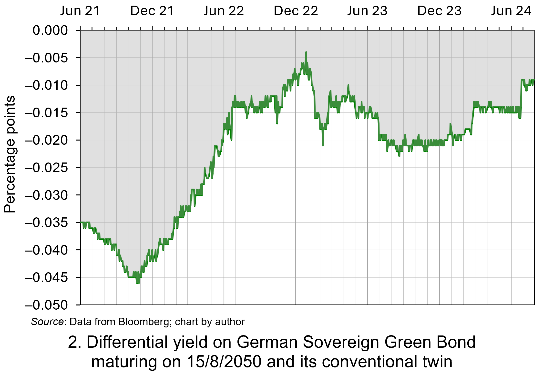 Figure 2 shows the difference in yields on a ‘green bond’ and its conventional counterpart, both maturing on 15/8/2050, between June 2021 and July 2024. The yield on the green bond is lower – on average about 2.2 basis points (0.022 percentage points) over the period. This represents the sacrifice in financial return that investors are prepared to trade off for higher environmental and social welfare in the future. (Click here for a PowerPoint.)
The yield spread fluctuates through time, reflecting changing perceptions of environmental concerns and hence the changing value that sustainable investors attach to future generations. The spread tends to widen when there are heightened environmental concerns and to narrow when such concerns are not in the news. For example, the spread on the twin German bonds reached a maximum of 0.045 percentage points in November 2021. This coincided with the 26th UN Climate Change Conference of the Parties (COP26) in Glasgow. The spread has narrowed significantly since early 2022 as rising interest rates and falling real rates of return on bonds in the near-term seem to have dominated investors’ concerns.
These data suggest that, rather than being too large, the greeniums are too small. The spreads suggest that markets in debt instruments do not seem to attach much value to future generations. The valuation, price and yield of green bonds are not significantly different from their conventional counterparts. This narrow gap indicates insufficient reward for better sustainability impact and little penalty for worse sustainability impact.
This pattern is repeated across financial markets and does not seem to be stimulating the necessary investment to achieve sustainable development. An estimate of the scale of the deficit in green financing is provided by Bloomberg NEF (2024). While global spending on the green energy transition reached $1.8 trillion in 2023, Bloomberg estimates that $4.8 trillion needs to be invested every year for the remainder of this decade if the world is to remain on track under the ‘net zero’ scenario. Investors do not seem to be prepared to accept the trade-off needed to provide the necessary funds.
Can financial markets deliver sustainable development?
Ultimately, the hope is that all financial instruments will be sustainable. In order to achieve that, access to finance would require all investors to incorporate the welfare of future generations in their investment decisions and accept sacrificing sufficient short-term financial return to ensure long-term sustainable development. Unfortunately, the pricing of green bonds suggests that investors are not prepared to accept the trade-off. This restricts the ability of financial markets to deliver an allocation of resources consistent with sustainable development.
There are several reasons why financial markets may not be valuing the welfare of future generations fully.
- Bounded rationality means that it is difficult for sustainable investors to assign precise values to future and distant benefits.
- There are no standardised sustainability metrics available. This produces great uncertainty in the valuation of future welfare.
- Investors also exhibit cognitive biases, which means they may not value the welfare of future generations properly. These include present bias (favouring immediate rewards) and hyperbolic discounting (valuing the near future more than the distant future).
- Economic models of financial valuation use discount rates to assess the value of future benefits. Higher discount rates reduce the perceived value of benefits occurring in the distant future. As a result, long-term impacts (such as environmental conservation) may be undervalued.
- There may be large numbers of investors who are only interested in financial returns and so do not consider the welfare of future generations in their investment decisions.
Consequently, investors need to be educated about the extent of trade-offs required to achieve the necessary investments in sustainable development. Furthermore, practical models which better reflect the welfare of future generations in investment decisions need to be employed. However, challenges persist in fully accounting for future generations and it may need regulatory frameworks to provide appropriate incentives for effective sustainable investment.
Articles
- The fallacy of ESG investing
Financial Times, Robert Armstrong (23/10/20)
- Energy Transition Investment Trends 2024: Executive Summary
BloombergNEF (30/1/24)
- ESG metrics trip up factor investors
Financial Times, Emma Boyde (1/11/21)
- Our Common Future: Report of the World Commission on Environment and Development
United Nations, Gro Harlem Brundtland (chair) (20/3/87)
 Who killed the ESG party?
FT Film, Daniel Garrahan (17/7/24)
- Green bond issuance surges as investors hunt for yield
Financial Times, Lee Harris (19/6/24)
- Investing for long-term value creation
Journal of Sustainable Finance & Investment, 9(4), Dirk Schoenmaker and Willem Schramade (19/6/19)
- Facts and Fantasies about the Green Bond Premium
Amundi working paper 102-2020, Mohamed Ben Slimane, Dany Da Fonseca and Vivek Mahtani (December 2020)
- Climate change and growth
Industrial and Corporate Change, 32 (2), 2023, Nicholas Stern and Joseph E Stiglitz (30/7/24)
Report
Data
Questions
- Using demand and supply analysis, illustrate and explain the impact of sustainable investing on the markets for (i) green bonds and (ii) conventional bonds. Highlight how this should produce an allocation of finance capital consistent with sustainable development.
- Research the yields on the twin bonds issued by Germany since this blog was published. Can you identify any association between heightened environmental concerns and the spread between the ‘green’ and conventional bond?
- Analyse the issues which prevent financial markets from producing the pricing signals which produce an allocation of resources consistent with sustainable development.
- Research some potential regulatory policies which may provide appropriate incentives for sustainable investment.
 The past decade or so has seen large-scale economic turbulence. As we saw in the blog Fiscal impulses, governments have responded with large fiscal interventions. The COVID-19 pandemic, for example, led to a positive fiscal impulse in the UK in 2020, as measured by the change in the structural primary balance, of over 12 per cent of national income.
The scale of these interventions has led to a significant increase in the public-sector debt-to-GDP ratio in many countries. The recent interest rates hikes arising from central banks responding to inflationary pressures have put additional pressure on the financial well-being of governments, not least on the financing of their debt. Here we discuss these pressures in the context of the ‘r – g’ rule of sustainable public debt.
Public-sector debt and borrowing
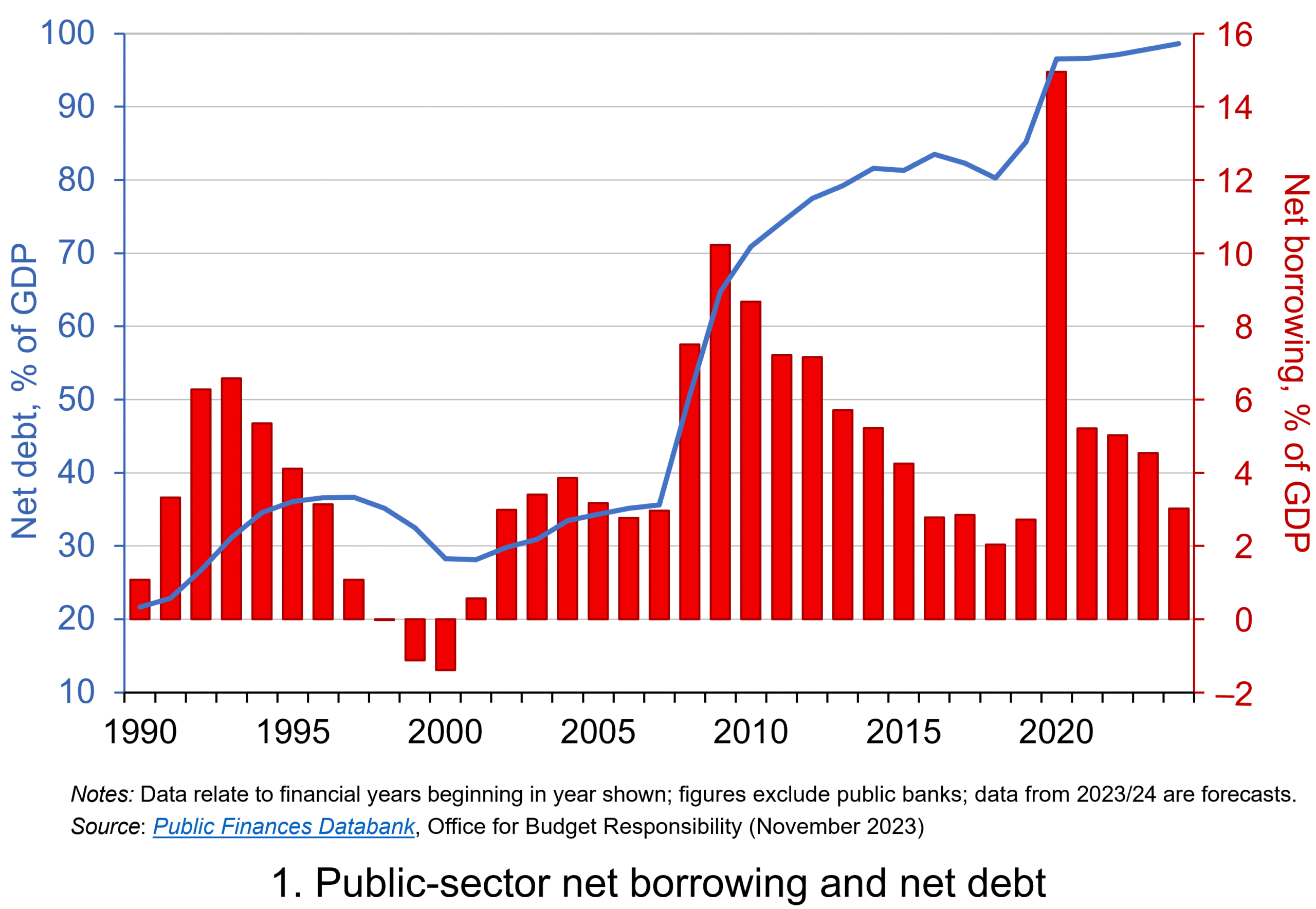 Chart 1 shows the path of UK public-sector net debt and net borrowing, as percentages of GDP, since 1990. Debt is a stock concept and is the result of accumulated flows of past borrowing. Net debt is simply gross debt less liquid financial assets, which mainly consist of foreign exchange reserves and cash deposits. Net borrowing is the headline measure of the sector’s deficit and is based on when expenditures and receipts (largely taxation) are recorded rather than when cash is actually paid or received. (Click here for a PowerPoint of Chart 1)
Chart 1 shows the impact of the fiscal interventions associated with the global financial crisis and the COVID-19 pandemic, when net borrowing rose to 10 per cent and 15 per cent of GDP respectively. The former contributed to the debt-to-GDP ratio rising from 35.6 per cent in 2007/8 to 81.6 per cent in 2014/15, while the pandemic and subsequent cost-of-living interventions contributed to the ratio rising from 85.2 per cent in 2019/20 to around 98 per cent in 2023/24.
Sustainability of the public finances
 The ratcheting up of debt levels affects debt servicing costs and hence the budgetary position of government. Yet the recent increases in interest rates also raise the costs faced by governments in financing future deficits or refinancing existing debts that are due to mature. In addition, a continuation of the low economic growth that has beset the UK economy since the global financial crisis also has implications for the burden imposed on the public sector by its debts, and hence the sustainability of the public finances. After all, low growth has implications for spending commitments, and, of course, the flow of receipts.
The analysis therefore implies that the sustainability of public-sector debt is dependent on at least three factors: existing debt levels, the implied average interest rate facing the public sector on its debts, and the rate of economic growth. These three factors turn out to underpin a well-known rule relating to the fiscal arithmetic of public-sector debt. The rule is sometimes known as the ‘r – g’ rule (i.e. the interest rate minus the growth rate).
Underpinning the fiscal arithmetic that determines the path of public-sector debt is the concept of the ‘primary balance’. This is the difference between the sector’s receipts and its expenditures less its debt interest payments. A primary surplus (a positive primary balance) means that receipts exceed expenditures less debt interest payments, whereas a primary deficit (a negative primary balance) means that receipts fall short. The fiscal arithmetic necessary to prevent the debt-to-GDP ratio rising produces the following stable debt equation or ‘r – g’ rule:

On the left-hand side of the stable debt equation is the required primary surplus (PS) to GDP (Y) ratio. Moving to the right-hand side, the first term is the existing debt-to-GDP ratio (D/Y). The second term ‘r – g’, is the differential between the average implied interest rate the government pays on its debt and the growth rate of the economy. These terms can be expressed in either nominal or real terms as this does not affect the differential.
To illustrate the rule consider a country whose existing debt-to-GDP ratio is 1 (i.e. 100 per cent) and the ‘r – g’ differential is 0.02 (2 percentage points). In this scenario they would need to run a primary surplus to GDP ratio of 0.02 (i.e. 2 percent of GDP).
The ‘r – g‘ differential
The ‘r – g’ differential reflects macroeconomic and financial conditions. The fiscal arithmetic shows that these are important for the dynamics of public-sector debt. The fiscal arithmetic is straightforward when r = g as any primary deficit will cause the debt-to-GDP ratio to rise, while a primary surplus will cause the ratio to fall. The larger is g relative to r the more favourable are the conditions for the path of debt. Importantly, if the differential is negative (r < g), it is possible for the public sector to run a primary deficit, up to the amount that the stable debt equation permits.
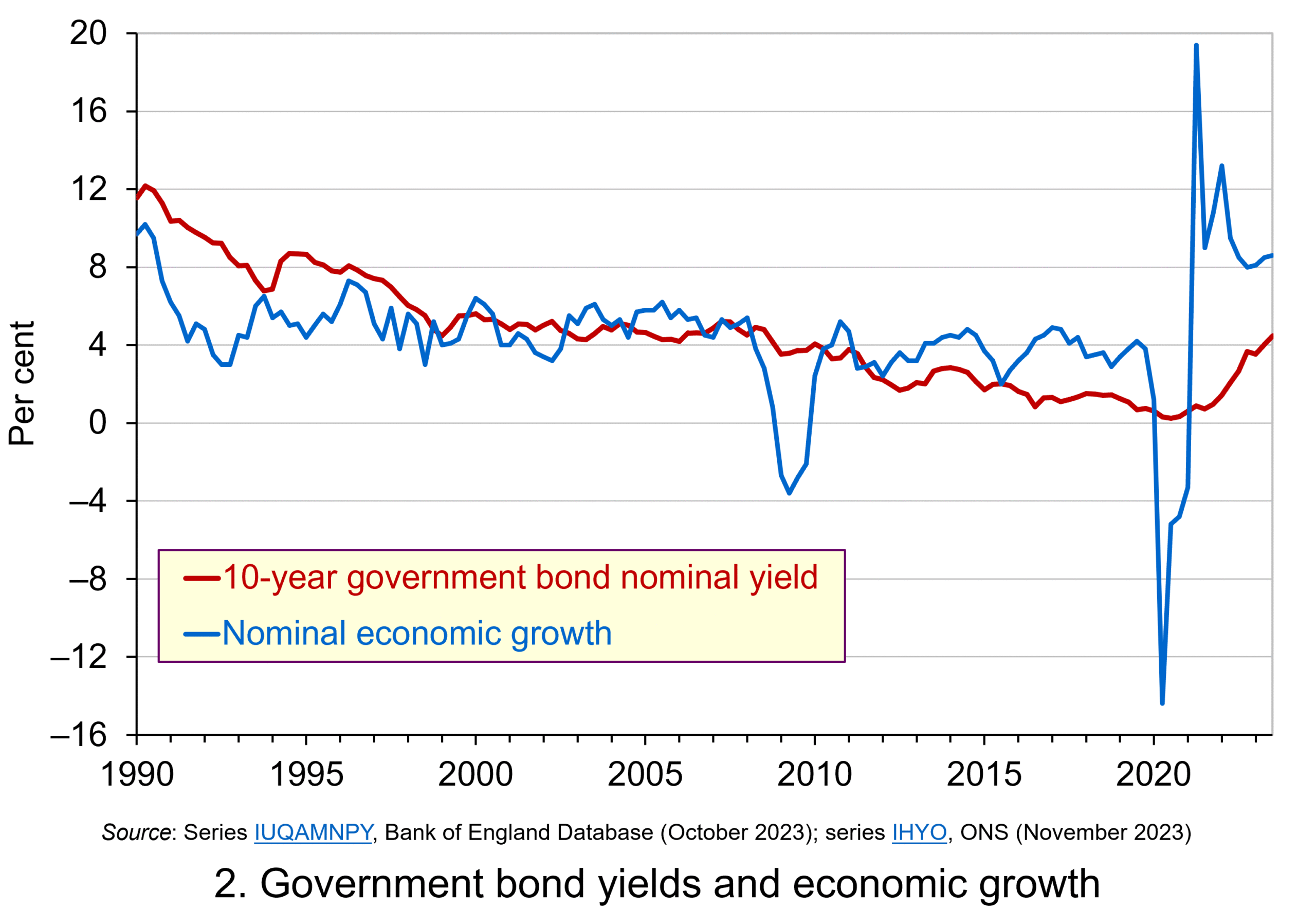 Consider Charts 2 and 3 to understand how the ‘r – g’ differential has affected debt sustainability in the UK since 1990. Chart 2 plots the implied yield on 10-year government bonds, alongside the annual rate of nominal growth (click here for a PowerPoint). As John explains in his blog The bond roller coaster, the yield is calculated as the coupon rate that would have to be paid for the market price of a bond to equal its face value. Over the period, the average annual nominal growth rate was 4.5 per cent, while the implied interest rate was almost identical at 4.6 per cent. The average annual rate of CPI inflation over this period was 2.8 per cent.
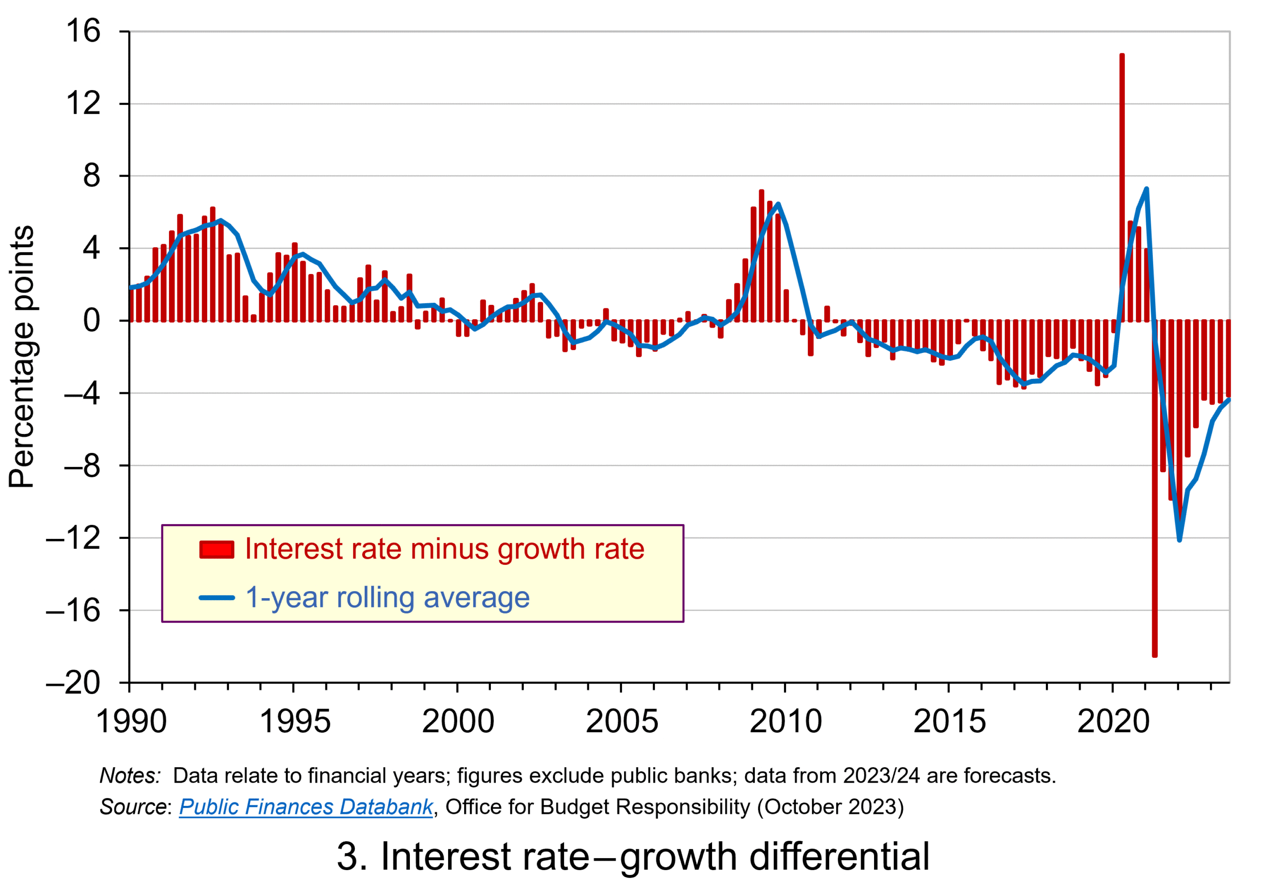 Chart 3 plots the ‘r – g’ differential which is simply the difference between the two series in Chart 2, along with a 12-month rolling average of the differential to help show better the direction of the differential by smoothing out some of the short-term volatility (click here for a PowerPoint). The differential across the period is a mere 0.1 percentage points implying that macroeconomic and financial conditions have typically been neutral in supporting debt sustainability. However, this does mask some significant changes across the period.
We observe a general downward trend in the ‘r – g’ differential from 1990 up to the time of the global financial crisis. Indeed between 2003 and 2007 we observe a favourable negative differential which helps to support the sustainability of public debt and therefore the well-being of the public finances. This downward trend of the ‘r – g’ differential was interrupted by the financial crisis, driven by a significant contraction in economic activity. This led to a positive spike in the differential of over 7 percentage points.
 Yet the negative differential resumed in 2010 and continued up to the pandemic. Again, this is indicative of the macroeconomic and financial environments being supportive of the public finances. It was, however, largely driven by low interest rates rather than by economic growth.
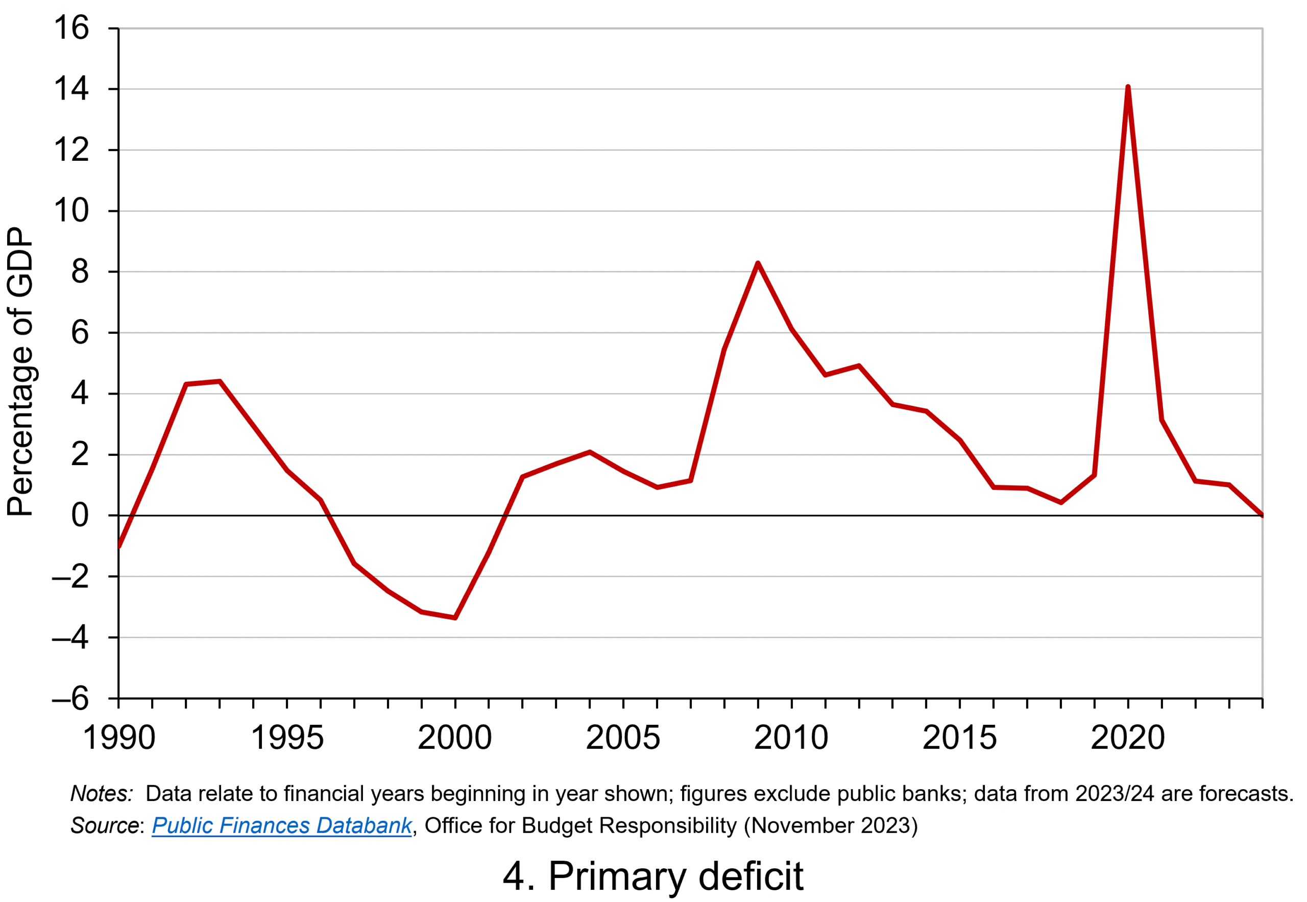
Consequently, the negative ‘r – g’ differential meant that the public sector could continue to run primary deficits during the 2010s, despite the now much higher debt-to-GDP ratio. Yet, weak growth was placing limits on this. Chart 4 indeed shows that primary deficits fell across the decade (click here for a PowerPoint).
The pandemic and beyond
 The pandemic saw the ‘r – g’ differential again turn markedly positive, averaging 7 percentage points in the four quarters from Q2 of 2020. While the differential again turned negative, the debt-to-GDP ratio had also increased substantially because of large-scale fiscal interventions. This made the negative differential even more important for the sustainability of the public finances. The question is how long the negative differential can last.
Looking forward, the fiscal arithmetic is indeed uncertain and worryingly is likely to be less favourable. Interest rates have risen and, although inflationary pressures may be easing somewhat, interest rates are likely to remain much higher than during the past decade. Geopolitical tensions and global fragmentation pose future inflationary concerns and a further drag on growth.
As well as the short-term concerns over growth, there remain long-standing issues of low productivity which must be tackled if the growth of the UK economy’s potential output is to be raised. These concerns all point to the important ‘r – g’ differential become increasingly less negative, if not positive. If so the fiscal arithmetic could mean increasingly hard maths for policymakers.
Articles
- The budget deficit: a short guide
House of Commons Library (8/6/23)
- If markets are right about long real rates, public debt ratios will increase for some time. We must make sure that they do not explode.
Peterson Institute for International Economics, Olivier Blanchard (6/11/23)
- The UK government’s debt nightmare
ITV News, Robert Peston (13/7/23)
- National debt could hit 300% of GDP by 2070s, independent watchdog the OBR warns
Sky News, James Sillars (13/7/23)
- How much money is the UK government borrowing, and does it matter?
BBC News (20/10/23)
- Cost of national debt hits 20-year high
BBC News, Vishala Sri-Pathma & Faisal Islam (4/10/23)
- Bond markets could see ‘mini boom-bust cycles’ as global government debt to soar by $5 trillion a yea
Markets Insider, Filip De Mott (16/11/23)
- The counterintuitive truth about deficits for bond investors
Financial Times, Matt King (17/11/23)
- UK government borrowing almost £20bn lower than expected
The Guardian, Richard Partington (20/10/23)
- Controlling debt is just a means — it is not a government’s end
Financial Times, Martin Wolf (13/11/23)
Data
Questions
- What is meant by each of the following terms: (a) net borrowing; (b) primary deficit; (c) net debt?
- Explain how the following affect the path of the public-sector debt-to-GDP ratio: (a) interest rates; (b) economic growth; (c) the existing debt-to-GDP ratio.
- Which factors during the 2010s were affecting the fiscal arithmetic of public debt positively, and which negatively?
- Discuss the prospects for the fiscal arithmetic of public debt in the coming years.
- Assume that a country has an existing public-sector debt-to-GDP ratio of 60 percent.
(a) Using the ‘rule of thumb’ for public debt dynamics, calculate the approximate primary balance it would need to run in the coming year if the expected average real interest rate on the debt were 3 per cent and real economic growth were 2 per cent?
(b) Repeat (a) but now assume that real economic growth is expected to be 4 per cent.
(c) Repeat (a) but now assume that the existing public-sector debt-to-GDP ratio is 120 per cent.
(d) Using your results from (a) to (c) discuss the factors that affect the fiscal arithmetic of the growth of public-sector debt.
 To finance budget deficits, governments have to borrow. They can borrow short-term by issuing Treasury bills, typically for 1, 3 or 6 months. These do not earn interest and hence are sold at a discount below the face value. The rate of discount depends on supply and demand and will reflect short-term market rates of interest. Alternatively, governments can borrow long-term by issuing bonds. In the UK, these government securities are known as ‘gilts’ or ‘gilt-edged securities’. In the USA they are known as ‘treasury bonds’, ‘T-bonds’ or simply ‘treasuries’. In the EU, countries separately issue bonds but the European Commission also issues bonds.
In the UK, gilts are issued by the Debt Management Office on behalf of the Treasury. Although there are index-linked gilts, the largest proportion of gilts are conventional gilts. These pay a fixed sum of money per annum per £100 of face value. This is known as the ‘coupon payment’ and the rate is set at the time of issue. The ‘coupon rate’ is the payment per annum as a percentage of the bond’s face value:

Payments are made six-monthly. Each issue also has a maturity date, at which point the bonds will be redeemed at face value. For example, a 4½% Treasury Gilt 2028 bond has a coupon rate of 4½% and thus pays £4.50 per annum (£2.25 every six months) for each £100 of face value. The issue will be redeemed in June 2028 at face value. The issue was made in June 2023 and thus represented a 5-year bond. Gilts are issued for varying lengths of time from 2 to 55 years. At present, there are 61 different conventional issues of bonds, with maturity dates varying from January 2024 to October 2073.
Bond prices
 Bonds can be sold on the secondary market (i.e. the stock market) before maturity. The market price, however, is unlikely to be the coupon price (i.e. the face value). The lower the coupon rate relative to current interest rates, the less valuable the bond will be. For example, if interest rates rise, and hence new bonds pay a higher coupon rate, the market price of existing bonds paying a lower coupon rate must fall. Thus bond prices vary inversely with interest rates.
The market price also depends on how close the bonds are to maturity. The closer the maturity date, the closer the market price of the bond will be to the face value.
Bond yields: current yield
A bond’s yield is the percentage return that a person buying the bond receives. If a newly issued bond is bought at the coupon price, its yield is the coupon rate.
However, if an existing bond is bought on the secondary market (the stock market), the yield must reflect the coupon payments relative to the purchase price, not the coupon price. We can distinguish between the ‘current yield’ and the ‘yield to maturity’.
The current yield is the coupon payment as a percentage of the current market price of the bond:

Assume a bond were originally issued at 2% (its coupon rate) and thus pays £2 per annum. In the meantime, however, assume that interest rates have risen and new bonds now have a coupon rate of 4%, paying £4 per annum for each £100 invested. To persuade people to buy old bonds with a coupon rate of 2%, their market prices must fall below their face value (their coupon price). If their price halved, then they would pay £2 for every £50 of their market price and hence their current yield would be 4% (£2/£50 × 100).
Bond yields: yield to maturity (YTM)
But the current yield does not give the true yield – it is only an approximation. The true yield must take into account not just the market price but also the maturity value and the length of time to maturity (and the frequency of payments too, which we will ignore here). The closer a bond is to its maturity date, the higher/lower will be the true yield if the price is below/above the coupon price: in other words, the closer will the market price be to the coupon price for any given market rate of interest.
A more accurate measure of a bond’s yield is thus the ‘yield to maturity’ (YTM). This is the interest rate which makes the present value of all a bond’s future cash flows equal to its current price. These cash flows include all coupon payments and the payment of the face value on maturity. But future cash flows must be discounted to take into account the fact that money received in the future is worth less than money received now, since money received now could then earn interest.
The yield to maturity is the internal rate of return (IRR) of the bond. This is the discount rate which makes the present value (PV) of all the bond’s future cash flows (including the maturity payment of the coupon price) equal to its current market price. For simplicity, we assume that coupon payments are made annually. The formula is the one where the bond’s current market price is given by:

Where: t is the year; n is the number of years to maturity; YTM is the yield to maturity.
Thus if a bond paid £5 each year and had a maturity value of £100 and if current interest rates were higher than 5%, giving a yield to maturity of 8%, then the bond price would be:

In other words, with a coupon rate of 5% and a higher YTM of 8%, the bond with a face value of £100 and five years to maturity would be worth only £88.02 today.
If you know the market price of a given bond, you can work out its YTM by substituting in the above formula. The following table gives examples.
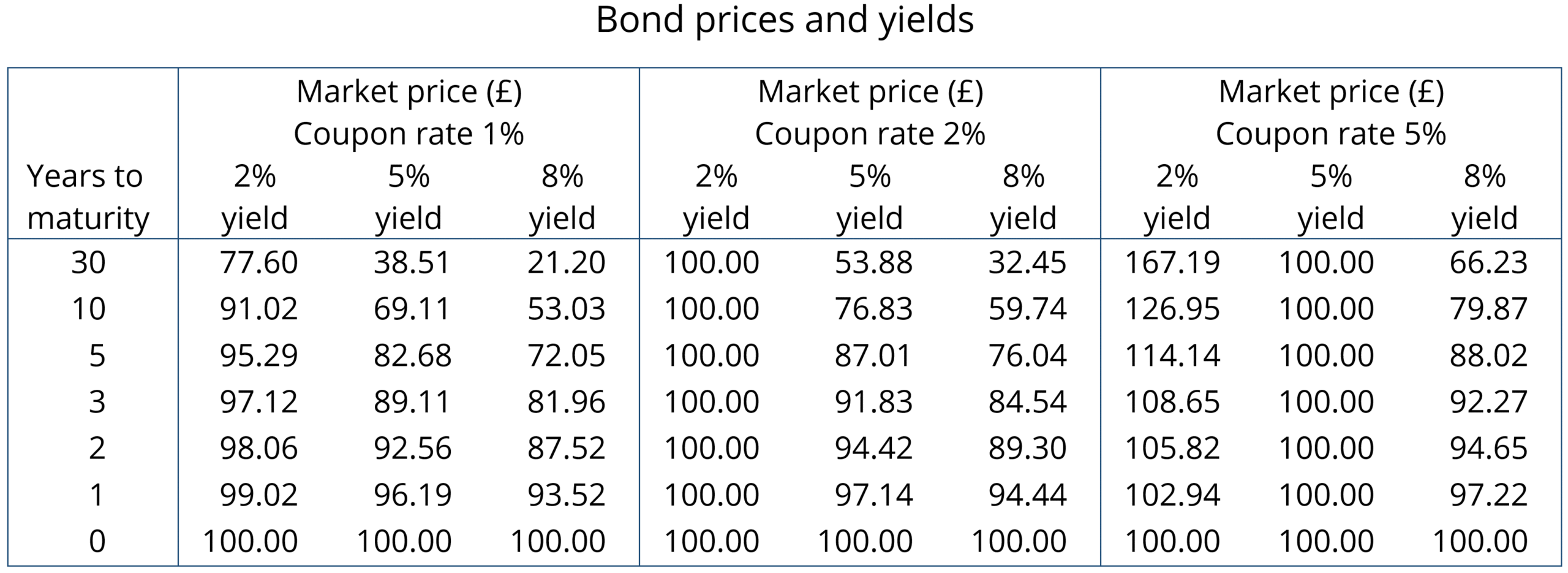
The higher the YTM, the lower the market price of a bond. Since the YTM reflects in part current rates of interest, so the higher the rate of interest, the lower the market price of any given bond. Thus bond yields vary directly with interest rates and bond prices vary inversely. You can see this clearly from the table. You can also see that market bond prices converge on the face value as the maturity date approaches.
Recent activity in bond markets
Investing in government bonds is regarded as very safe. Coupon payments are guaranteed, as is repayment of the face value on the maturity date. For this reason, many pension funds hold a lot of government bonds issued by financially trustworthy governments. But in recent months, bond prices in the secondary market have fallen substantially as interest rates have risen. For those holding existing bonds, this means that their value has fallen. For governments wishing to borrow by issuing new bonds, the cost has risen as they have to offer a higher coupon rate to attract buyers. This make it more expensive to finance government debt.
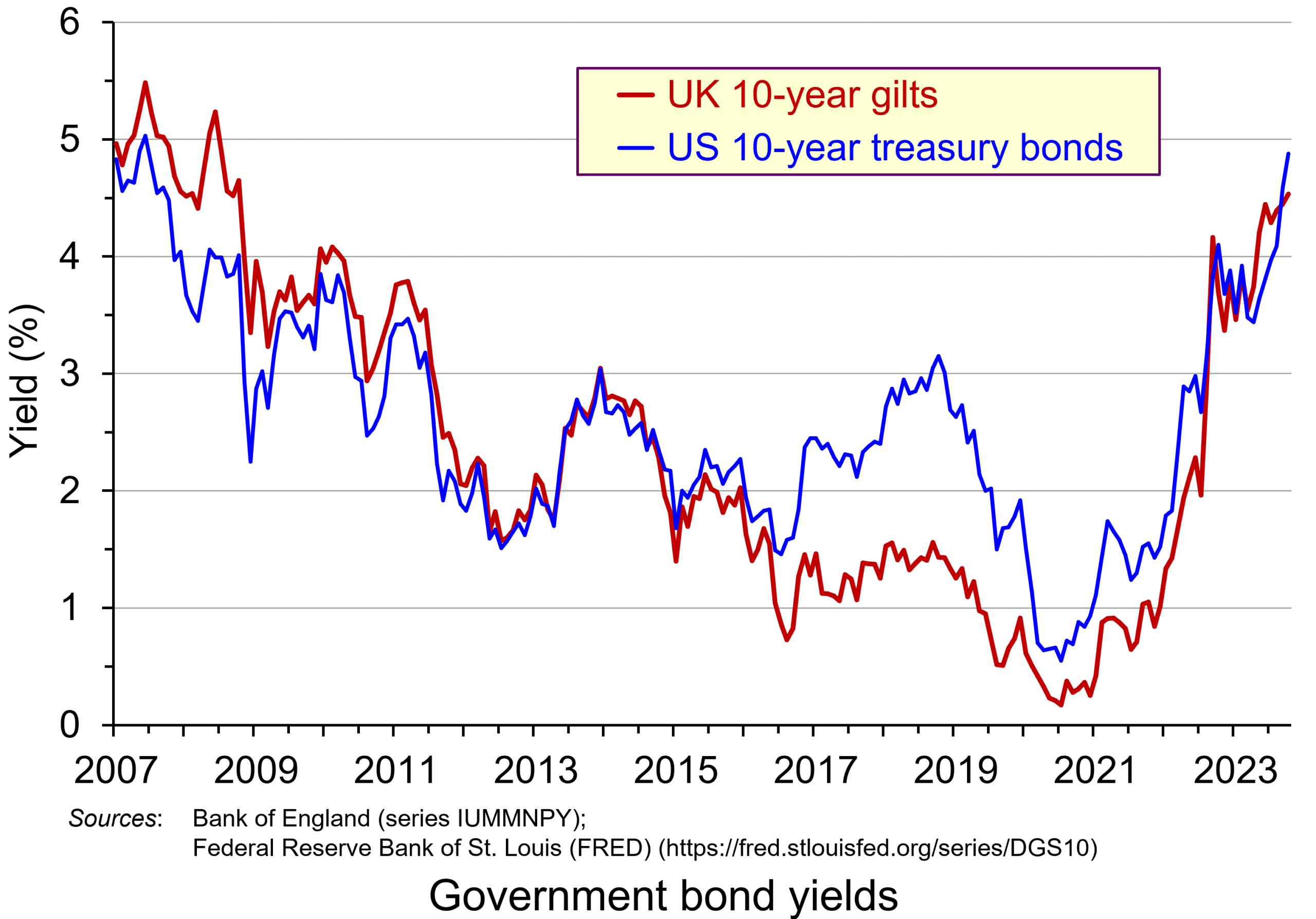 The chart shows the yield on 10-year government bonds. It is calculated using the ‘par value’ approach. This gives the coupon rate that would have to be paid for the market price of a bond to equal its face value. Clearly, as interest rates rise, a bond would have to pay a higher coupon rate for this to happen. (This, of course, is only hypothetical to give an estimate of market rates, as coupon rates are fixed at the time of a bond’s issue.)
Par values reflect both yield to maturity and also expectations of future interest rates. The higher people expect future interest rates to be, the higher must par values be to reflect this.
 In the years following the financial crisis of 2007–8 and the subsequent recession, and again during the COVID pandemic, central banks cut interest rates and supported this by quantitative easing. This involved central banks buying existing bonds on the secondary market and paying for them with newly created (electronic) money. This drove up bond prices and drove down yields (as the chart shows). This helped support the policy of low interest rates. This was a boon to governments, which were able to borrow cheaply.
This has all changed. With quantitative tightening replacing quantitative easing, central banks have been engaging in asset sales, thereby driving down bond prices and driving up yields. Again, this can be seen in the chart. This has helped to support a policy of higher interest rates.
Problems of higher bond yields/lower bond prices
Although lower bond prices and higher yields have supported a tighter monetary policy, which has been used to fight inflation, this has created problems.
First, it has increased the cost of financing government debt. In 2007/8, UK public-sector net debt was £567bn (35.6% of GDP). The Office for Budget Responsibility forecasts that it will be £2702bn (103.1% of GDP in the current financial year – 2023/24). Not only, therefore, are coupon rates higher for new government borrowing, but the level of borrowing is now a much higher proportion of GDP. In 2020/21, central government debt interest payments were 1.2% of GDP; by 2022/23, they were 4.4% (excluding interest on gilts held in the Bank of England, under the Asset Purchase Facility (quantitative easing)).
 In the USA, there have been similar increases in government debt and debt interest payments. Debt has increased from $9tn in 2007 to $33.6tn today. Again, with higher interest rates, debt interest as a percentage of GDP has risen: from 1.5% of GDP in 2021 to a forecast 2.5% in 2023 and 3% in 2024. What is more, 31 per cent of US government bonds will mature next year and will need refinancing – at higher coupon rates.
There is a similar picture in other developed countries. Clearly, higher interest payments leave less government revenue for other purposes, such as health and education.
Second, many pension funds, banks and other investment companies hold large quantities of bonds. As their price falls, so this reduces the value of these companies’ assets and makes it harder to finance new purchases, or payments or loans to customers. However, the fact that new bonds pay higher interest rates means that when existing bond holdings mature, the money can be reinvested at higher rates.
Third, bonds are often used by companies as collateral against which to borrow and invest in new capital. As bond prices fall, this can hamper companies’ ability to invest, which will lead to lower economic growth.
Fourth, higher bond yields divert demand away from equities (shares). With equity markets falling back or at best ceasing to rise, this erodes the value of savings in equities and may make it harder for firms to finance investment through new issues.
At the core of all these problems is inflation and budget deficits. Central banks have responded by raising interest rates. This drives up bond yields and drives down bond prices. But bond prices and yields depend not just on current interest rates, but also on expectations about future interest rates. Expectations currently are that budget deficits will be slow to fall as governments seek to support their economies post-COVID. Also expectations are that inflation, even though it is falling, is not falling as fast as originally expected – a problem that could be exacerbated if global tensions increase as a result of the ongoing war in Ukraine, the Israel/Gaza war and possible increased tensions with China concerning disputes in the China Sea and over Taiwan. Greater risks drive up bond yields as investors demand a higher interest premium.
Articles
Information and data
Questions
- Why do bond prices and bond yields vary inversely?
- How are bond yields and prices affected by expectations?
- Why are ‘current yield’ and ‘yield to maturity’ different?
- What is likely to happen to bond prices and yields in the coming months? Explain your reasoning.
- What constraints do bond markets place on fiscal policy?
- Would it be desirable for central banks to pause their policy of quantitative tightening?
 The gold market has become one of the most talked-about commodity markets in 2025, with prices reaching record highs. This is largely due to increased demand from investors, who see gold as a ‘safe haven’ during times of economic and political uncertainty. Central banks are also buying more gold as a way to reduce their reliance on currencies like the US dollar. With many analysts predicting prices could reach over $4000 per ounce in the next year, the gold market is showcasing how supply and demand, confidence, and global events can all influence a commodity market.
 This year, the gold market has seen a remarkable rally, with the price of gold hitting a record high. Demand for the precious metal has resulted in spot prices surging over 35% to date (see the chart: click here for a PowerPoint). Rising prices earlier this year have been attributed to the US President, Donald Trump, announcing wide-ranging tariffs which have upset global trade. On 2 September, the spot gold price hit $3508.50 per ounce, continuing its upwards trend.
 The rise in the price of gold by more than a third this year can be linked to the US election last year, according to the director of research at BullionVault (see the BBC article below). Attitudes of the Trump administration towards the Federal Reserve have created concerns among investors. Fears that the US administration could erode the independence of the world’s most important central bank have fuelled the latest flows into the metal, which is traditionally viewed as a hedge against inflation.
  If the Federal Reserve does come under political pressure, it could affect the stability of the US economy and beyond. When gold prices rise sharply, demand usually falls in countries like China and India, which are the world’s largest buyers of gold jewellery. However, in 2025, this trend has changed. Instead of reducing their gold purchases, people in these countries have started buying investment gold, such as bars and coins, showing a shift in consumer behaviour from jewellery to investment assets.
 The foundation of gold’s rally to historic highs started back in 2022
 On 25 October 2024, Moody’s, one of the major credit ratings agencies, announced that it was downgrading France’s economic outlook to negative. This was its first downgrading of France since 2012. It followed a similar revision by Fitch’s, another ratings agency, on 11 October.
 The yield on 10-year French government debt began 2024 at 2.56% and had an upward trend for the first half of the year. The yield peaked at 3.34% on 1 July. It then fell back below 3% for a while. The negative economic outlook then pushed yields back above 3% and they finished October at 3.12%, half a percentage point above the level at the start of the year. This represents a significant increase in borrowing costs for the French government.
 If the expected rate of return rises, this increases the discount rate applied to future cash flows and reduces their present value. At the current price, the fixed coupon is not sufficient to compensate investors. So, investors sell the bonds and price falls until it reaches a point where the yield offered is equal to that required. The reverse happens if the expected rate of return falls.
  Governments in France last achieved a balanced budget in 1974. They have run deficits ever since. Figure 2 illustrates the French government budget deficits from 1990 to 2023 (click
  Further, political instability has grown due to the inconclusive parliamentary elections which Emmanuel Macron surprisingly called in July. No single political grouping has a majority and the President has appointed a Centrist Prime Minister, Michel Barnier (the former EU Brexit negotiator). His government is trying to pass a budget through the Assemblée Nationale involving a mixture of spending cuts and tax hikes which amount to savings of €60 billion ($66 billion). This is equivalent to 2% of GDP.
 In the past, bond investors were more tolerant of France’s budget deficits. French government bonds were attractive options for investors wanting to hold euro-denominated bonds while avoiding riskier Southern European countries such as Greece, Italy, Portugal and Spain. Since France has run persistent government deficits for a long time, it offered bond investors a more liquid market than more fiscally-parsimonious Northern European neighbours, such as Germany and the Netherlands. Consequently, France’s debt instruments offered a slight risk premium on the yields for those countries.
  As Figure 3 illustrates, this was the culmination of a trend evident throughout 2024, with the difference in yields between the two declining steadily (click
  Sustainability has become one of the most pressing issues facing society. Patterns of human production and consumption have become unsustainable. On the environmental front, climate change, land-use change, biodiversity loss and depletion of natural resource are destabilising the Earth’s eco-system.
 Sustainable finance has grown rapidly over the past decade as concerns about climate change have intensified. A significant element of this growth has been in global debt markets.
 Let’s trace the process. In models of sustainable finance, financial instruments such as green bonds funding investments with positive environmental impacts (such as renewable energy) should be valued more, while instruments funding investments with negative environmental impacts (such as fossil fuels) should be valued less. The prices of the green bonds financing renewable energy projects should rise while the prices of conventional bonds financing fossil-fuel companies should fall.
 Figure 2 shows the difference in yields on a ‘green bond’ and its conventional counterpart, both maturing on 15/8/2050, between June 2021 and July 2024. The yield on the green bond is lower – on average about 2.2 basis points (0.022 percentage points) over the period. This represents the sacrifice in financial return that investors are prepared to trade off for higher environmental and social welfare in the future. (Click
 The past decade or so has seen large-scale economic turbulence. As we saw in the blog
  Chart 1 shows the path of UK public-sector net debt and net borrowing, as percentages of GDP, since 1990. Debt is a stock concept and is the result of accumulated flows of past borrowing. Net debt is simply gross debt less liquid financial assets, which mainly consist of foreign exchange reserves and cash deposits. Net borrowing is the headline measure of the sector’s deficit and is based on when expenditures and receipts (largely taxation) are recorded rather than when cash is actually paid or received. (Click
  The ratcheting up of debt levels affects debt servicing costs and hence the budgetary position of government. Yet the recent increases in interest rates also raise the costs faced by governments in financing future deficits or refinancing existing debts that are due to mature. In addition, a continuation of the low economic growth that has beset the UK economy since the global financial crisis also has implications for the burden imposed on the public sector by its debts, and hence the sustainability of the public finances. After all, low growth has implications for spending commitments, and, of course, the flow of receipts.
 Consider Charts 2 and 3 to understand how the ‘r – g’ differential has affected debt sustainability in the UK since 1990. Chart 2 plots the implied yield on 10-year government bonds, alongside the annual rate of nominal growth (click
  Chart 3 plots the ‘r – g’ differential which is simply the difference between the two series in Chart 2, along with a 12-month rolling average of the differential to help show better the direction of the differential by smoothing out some of the short-term volatility (click
  Yet the negative differential resumed in 2010 and continued up to the pandemic. Again, this is indicative of the macroeconomic and financial environments being supportive of the public finances. It was, however, largely driven by low interest rates rather than by economic growth.
  The pandemic saw the ‘r – g’ differential again turn markedly positive, averaging 7 percentage points in the four quarters from Q2 of 2020. While the differential again turned negative, the debt-to-GDP ratio had also increased substantially because of large-scale fiscal interventions. This made the negative differential even more important for the sustainability of the public finances. The question is how long the negative differential can last.
 To finance budget deficits, governments have to borrow. They can borrow short-term by


 The chart shows the yield on 10-year government bonds. It is calculated using the ‘par value’ approach. This gives the coupon rate that would have to be paid for the market price of a bond to equal its face value. Clearly, as interest rates rise, a bond would have to pay a higher coupon rate for this to happen. (This, of course, is only hypothetical to give an estimate of market rates, as coupon rates are fixed at the time of a bond’s issue.)
  In the years following the financial crisis of 2007–8 and the subsequent recession, and again during the COVID pandemic, central banks cut interest rates and supported this by quantitative easing. This involved central banks buying existing bonds on the secondary market and paying for them with newly created (electronic) money. This drove up bond prices and drove down yields (as the chart shows). This helped support the policy of low interest rates. This was a boon to governments, which were able to borrow cheaply.
 In the USA, there have been similar increases in government debt and debt interest payments. Debt has increased from $9tn in 2007 to $33.6tn today. Again, with higher interest rates, debt interest as a percentage of GDP has risen: from 1.5% of GDP in 2021 to a forecast 2.5% in 2023 and 3% in 2024. What is more, 31 per cent of US government bonds will mature next year and will need refinancing – at higher coupon rates.