 On 25 October 2024, Moody’s, one of the major credit ratings agencies, announced that it was downgrading France’s economic outlook to negative. This was its first downgrading of France since 2012. It followed a similar revision by Fitch’s, another ratings agency, on 11 October.
While Fitch’s announcement did not have a significant impact on the yields of French government bonds, expectations around Moody’s did. In the week preceding the announcement, the net increases in the yield on generic 10-year government debt was approximately 9 basis points (0.09 percentage points). On the day itself, the yield rose by approximately 5.6 basis points (0.056 percentage points).
The yield rose further throughout the rest of October, finishing nearly 0.25 percentage points above its level at the start of the month. However, as Figure 1 illustrates, these increases are part of a longer-term trend of rising yields for French government debt (click here for a PowerPoint).
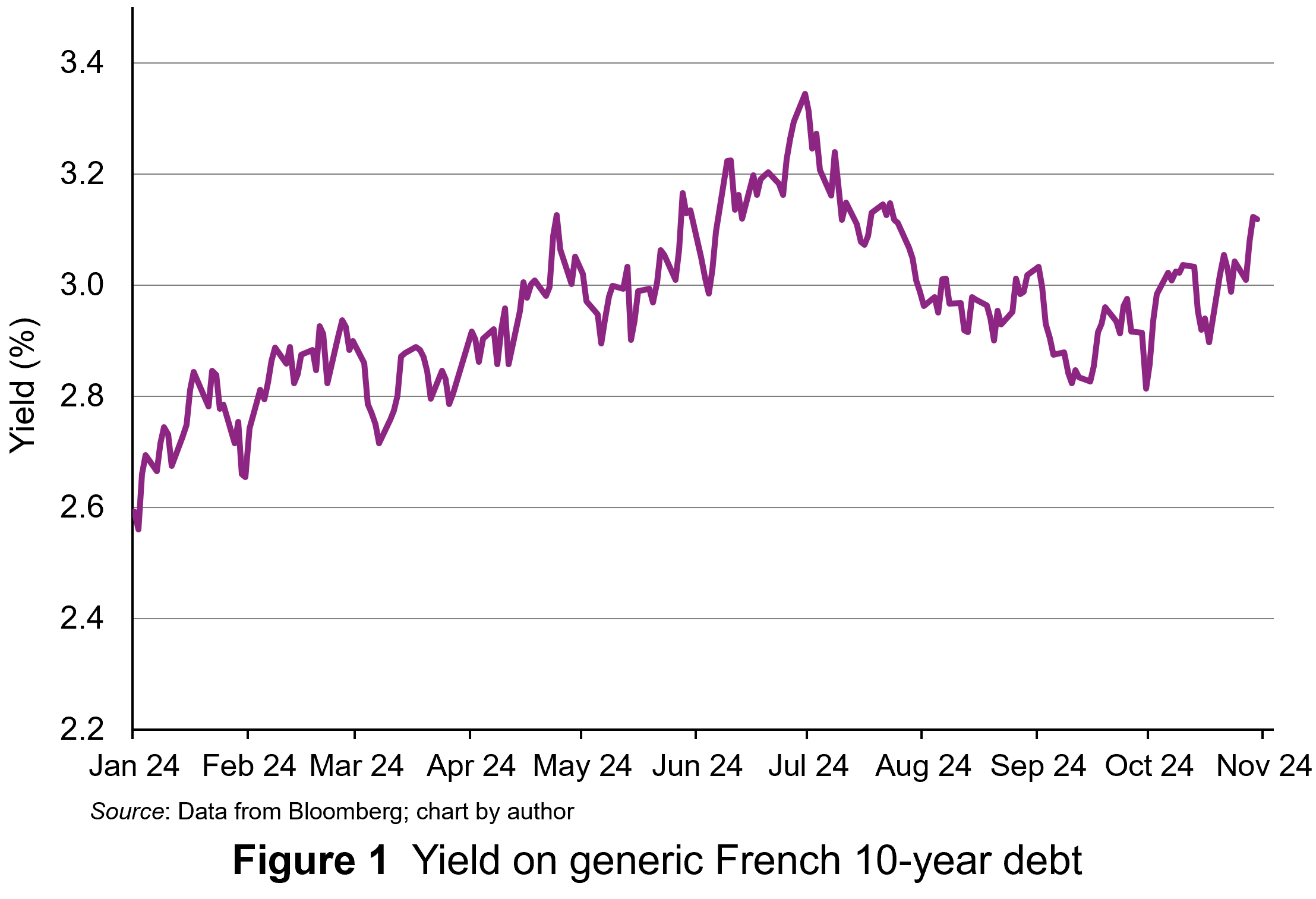 The yield on 10-year French government debt began 2024 at 2.56% and had an upward trend for the first half of the year. The yield peaked at 3.34% on 1 July. It then fell back below 3% for a while. The negative economic outlook then pushed yields back above 3% and they finished October at 3.12%, half a percentage point above the level at the start of the year. This represents a significant increase in borrowing costs for the French government.
In this blog, we will explain why the changes in France’s economic outlook translate into increases in yields for French government bonds. We will also analyse why yields have increased and examine the prospects for the markets in French government bonds.
Pricing signals of bond yields
A bond is a tradable debt instrument issued by governments to finance budget deficits – the difference between tax receipts and spending. Like any financial instruments, investment in bonds involves a commitment of funds today in anticipation of interest payments through time as compensation, with a repayment of its redemption value on the date the bond matures.
Since the cash flows associated with holding a bond occur at different points in time, discounted cash flow analysis is used to determine its value. This gives the present value of the cash flows discounted at the appropriate expected rate of return. In equilibrium this will be equal to the bond’s market price, as the following equation shows.

Where:
P = the equilibrium price of the bond
C = cash coupon payments
M = redemption value at maturity
r = yield (expected rate of return in equilibrium.
Interest payments tend to be fixed at the time a bond is issued and reflect investors’ expected rate of return, expressed as the yield in bond markets. This is determined by prevailing interest rates and perceived risk. Over time, changes in interest rates and perceptions of risk will change the expected rate of return (yield), which will, in turn, change the present value of the cash flows, and hence fundamental value.
Prices move in response to changes in fundamental value and since this happens frequently, this means that prices change a lot. For bonds, as the coupon payments (C each year and the redemption price () are fixed, the only factor that can change is the expected rate of return (yield). This is reflected in the observed yield at each price.
 If the expected rate of return rises, this increases the discount rate applied to future cash flows and reduces their present value. At the current price, the fixed coupon is not sufficient to compensate investors. So, investors sell the bonds and price falls until it reaches a point where the yield offered is equal to that required. The reverse happens if the expected rate of return falls.
The significant risk associated with bonds is credit default risk – the risk that the debt will not be repaid. The potential for credit default is a significant influence of the compensation investors require for holding debt instruments like bonds (ceteris paribus). An increase in expected credit default risk will increase the expected return (compensation). This will be reflected in a lower price and higher yield.
Normally, with the bonds issued by high-income countries, such as those in Europe and North America, the risk of default is extremely low. However, if a country’s annual deficits or accumulated debt increase to what markets consider to be unsustainable levels, the perceived risk of default may rise. Countries’ levels of risk are rated by international ratings agencies, such as Moody’s and Fitch. Investors pay a lot of attention to the information provided by such agencies.
Moody’s downgrade in its economic outlook for France from ‘stable’ to ‘negative’ indicated weak economic performance and higher credit default risk. This revision rippled through bond markets as investors adjusted their views of the country’s economic risk. The rise in yields observed is a signal that bond investors perceive higher credit default risk associated with French government debt and are demanding a higher rates of return as compensation.
Why has France’s credit default risk premium risen now?
As we have seen, credit default risk is not normally considered a significant issue for sovereign borrowers like France. Some of the issue around perceived credit default risk for the French government relate to the size of the French government’s deficit and the projections for it. Following a spike in borrowing associated with the COVID-19 pandemic in 2020, the annual government budget deficit and the overall level of debt as percentages of GDP have remained high. The annual deficit is projected to be 6% for 2024 and still 5% for 2025. The ratio of outstanding French government debt to Gross Domestic Product (GDP) ballooned to 123% in 2020 and is still expected to be 115% by the end of 2025. France has been put on notice to reduce its debt towards the Eurozone limit of 60% of GDP.
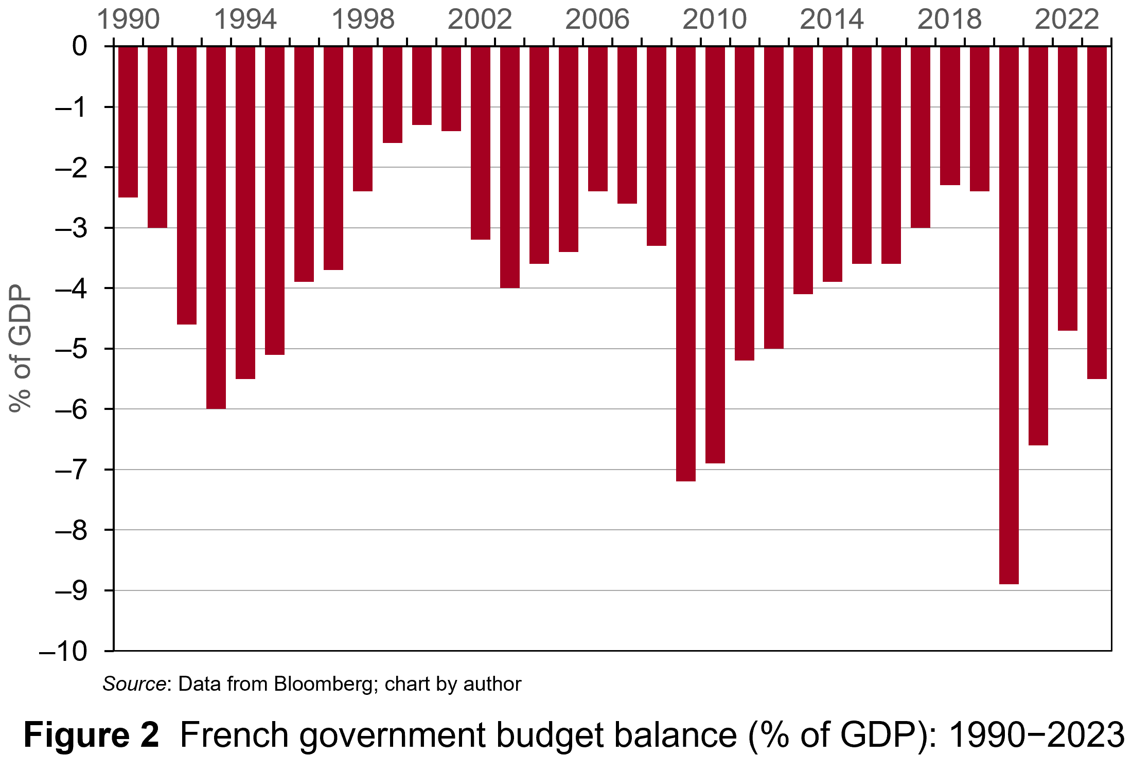 Governments in France last achieved a balanced budget in 1974. They have run deficits ever since. Figure 2 illustrates the French government budget deficits from 1990 to 2023 (click here for a PowerPoint). The figure shows that France experienced deficits in the past similar to today’s. These, however, did not tend to worry bond markets too much.
So why are investors currently worried? This stems from France’s debt mountain and from concerns that the government will not be able to deal with it. Investors are concerned that both weak growth and increasingly volatile politics will thwart efforts to reduce debt levels.
Let’s take growth. Even by contemporary European standards, France’s growth prospects are anaemic. GDP is expected to grow by just 1.1% for 2024 and 1% for 2025. Both consumer and business confidence are low. None of this suggests a growth spurt soon which will boost the tax revenues of the French government sufficiently to address the deficit.
 Further, political instability has grown due to the inconclusive parliamentary elections which Emmanuel Macron surprisingly called in July. No single political grouping has a majority and the President has appointed a Centrist Prime Minister, Michel Barnier (the former EU Brexit negotiator). His government is trying to pass a budget through the Assemblée Nationale involving a mixture of spending cuts and tax hikes which amount to savings of €60 billion ($66 billion). This is equivalent to 2% of GDP.
The parliamentary path of the budget bill is set to be torturous with both the left and right wing blocs in the Assemblée opposing most of the provisions. Debate in the Assemblée Nationale and Senate are expected to drag on into December, with the real prospect that the government may have to use presidential decree to pass the budget. Commentators argue that this will fuel further political chaos.
France looks more like Southern Europe
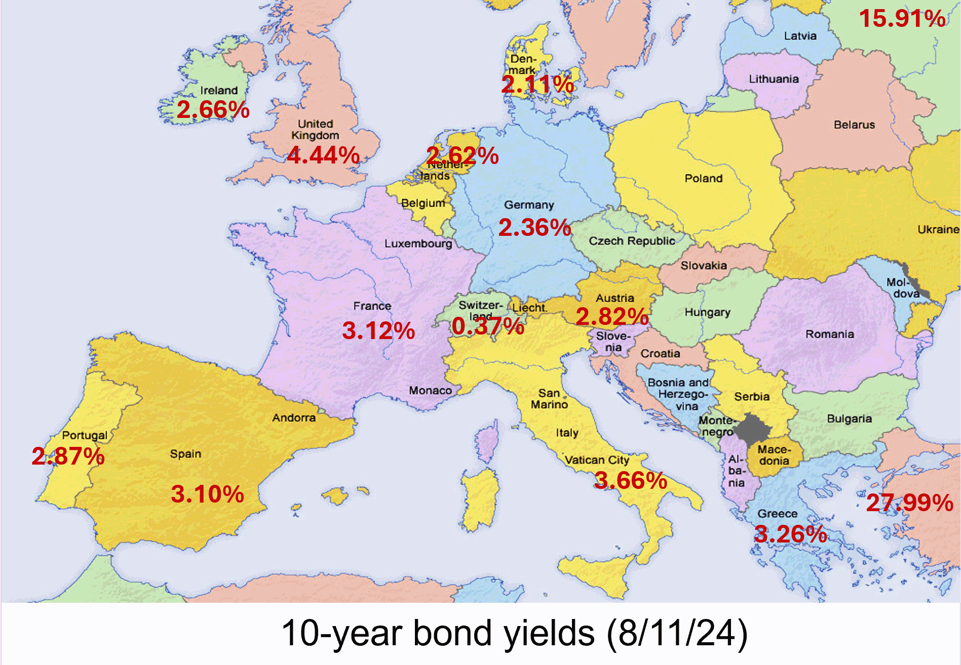 In the past, bond investors were more tolerant of France’s budget deficits. French government bonds were attractive options for investors wanting to hold euro-denominated bonds while avoiding riskier Southern European countries such as Greece, Italy, Portugal and Spain. Since France has run persistent government deficits for a long time, it offered bond investors a more liquid market than more fiscally-parsimonious Northern European neighbours, such as Germany and the Netherlands. Consequently, France’s debt instruments offered a slight risk premium on the yields for those countries.
However, that has changed. France’s credit default risk premium is rising to levels comparable to its Southern neighbours. On 26 September 2024, the yield on generic French government 10-year debt rose above its Spanish equivalent for the first time since 2008.
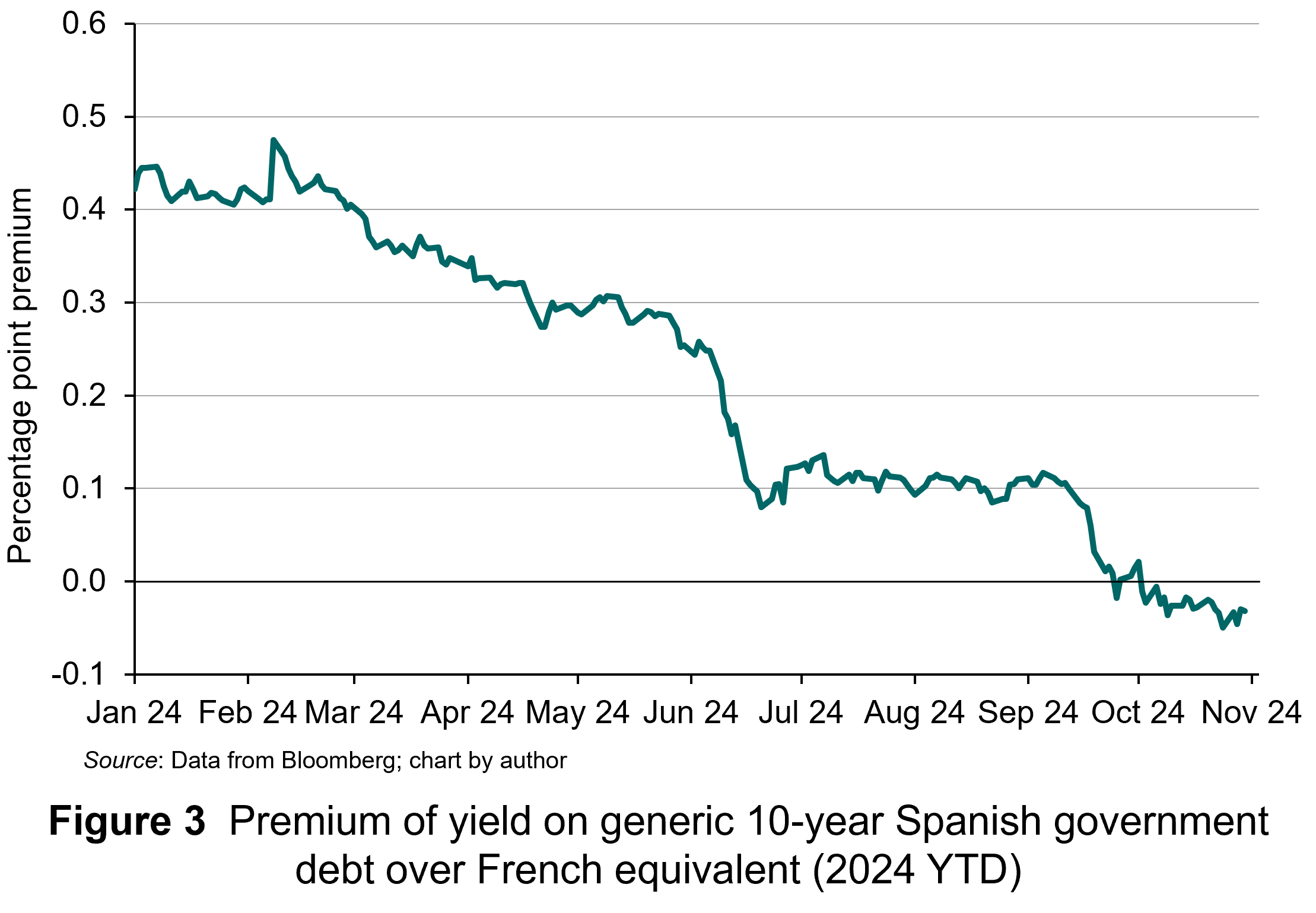 As Figure 3 illustrates, this was the culmination of a trend evident throughout 2024, with the difference in yields between the two declining steadily (click here for a PowerPoint). At the start of the year, the yield on Spanish debt offered a 40 basis points premium over the French equivalent. By October, the yield on Spanish debt was consistently below that of French debt. All of this is due to bond investors’ rising expectations about France’s credit default risk. Now, France’s borrowing costs are not only above Spain, but also closer to those of Greece and Italy than of Germany.
Strikingly, Spain’s budget deficit was 3.5% in 2023 and is expected to narrow to 2.6% by 2025. The percentage of total debt to GDP is 104% and falling. Moreover, following Spain’s inconclusive election in 2023, the caretaker government put forward budgetary plans involving fiscal tightening without the need for legislation. This avoided the political wrangling France is facing.
For France, these developments raise the prospect of yields rising further as bond investors now see alternatives to French government debt in the form of Spain’s. This country have already undertaken the painful fiscal adjustments that France seems incapable of completing.
Articles
Data
Questions
- What is credit default risk?
- Explain why higher credit default risk is associated with higher yields on France’s government debt.
- Why would low economic growth worsen the government’s budget deficit?
- Why would political instability increase credit default risk?
- What has happened to investors’ perceptions of the risk associated with French government debt relative to Spain’s?
- How has this manifested itself in the relative yields of the two countries’ government debt?
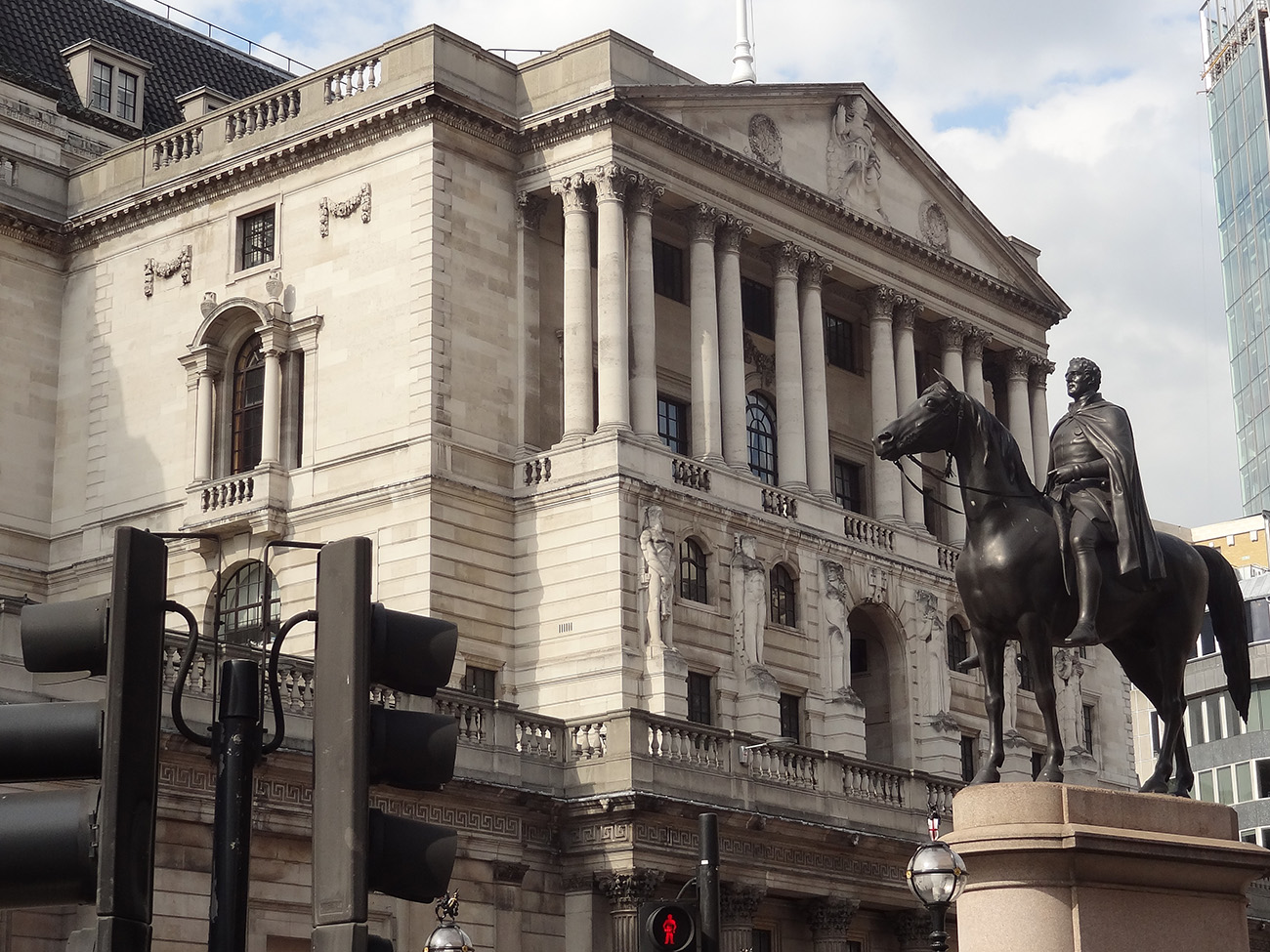 The UK government announced on 14 October 2024 in a ministerial statement that it intended to raise the threshold for the ring-fencing (separation) of retail and investment banking activities of large UK-based banks. These banks are known as ‘systemically important financial institutions (SIFIs)’, which are currently defined as those with more than £25bn of core retail deposits. Under the new regulations, the threshold would rise from £25bn to £35bn.
Ring-fencing is the separation of one set of banking services from another. This separation can be geographical or functional. The UK adopted the latter approach, where ring-fencing is the separation of core retail banking services, such as taking deposits, making payments and granting loans to small and medium-sized enterprises (SMEs) from investment banking and international operations. The intention of ring-fencing was to prevent contagion – to protect essential retail banking services from the risks involved in investment banking activities.
Reducing regulation to increase competition
Raising the limit is intended to facilitate greater competition in the retail banking sector. In recent years, US banks, such as JP Morgan and Goldman Sachs, have been expanding their depositor base in the UK under their respective brands – Chase UK and Marcus.
These relatively small UK subsidiaries were not ring-fenced from their wider investment banking operations as their retail deposits were under (but not far under) the £25bn limit. However, this restricted their ability to increase market share further without bearing the additional regulatory burden associated with ring-fencing that much larger incumbents face. Raising the threshold would allow them to expand to the higher limit without the regulatory burden.
The proposals are part of a broader package of reforms aimed at reducing the regulatory burden on UK-based banks. The hope is that this will stimulate greater lending to SMEs to boost investment and productivity.
The proposals also include a new ‘secondary’ threshold. This will exempt banks providing primarily retail banking services from the rules governing the provision of investment banking accounts. This exemption will apply as long as their investment banking is less than 10% of their tier 1 capital. (Tier 1 capital is currently the buffer which banks are required to retain in case of a crisis.) The changes were the outcome of a review conducted in 2022 but had not been implemented by the previous government.
The announcement has sparked a debate about ring-fencing, with some commentators calling for it to be removed altogether. Therefore, it is timely to revisit the rationale for ring-fencing. This blog examines what ring-fencing is and why it was introduced, and explains the associated economic costs and benefits.
Why was ring-fencing introduced?
 Ring-fencing was recommended by the Independent Commission on Banking (ICB) in 2011 (see link below) and implemented through the Financial Services (Banking Reform) Act of 2013. The proposed separation of core retail banking services from investment banking were intended to address issues in banks which arose during the global financial crisis and which required substantial taxpayer bailouts. (See the 2011 blog, Taking the gambling out of high street banking (update).)
Following deregulation and liberalisation of financial services in the 1980s, many UK banks had extended their operations so that they combined domestic retail operations with substantial investment and international operations. The intention was to open up all dimensions of financial services to greater competition and allow banks to exploit economies of scope between retail and investment banking.
However, the risks associated with these services are very different but, in the period before the financial crisis, were provided alongside one another within banking groups.
One significant risk which was not fully recognised at the time was contagion – problems in one dimension of a bank’s activity could severely compromise its ability to provide services in other areas. This is what happened during the financial crisis. Many of the UK banks’ investment operations had made significant investments in off-balance sheet securitised debt instruments – CDOs being the most famous example. (See the 2018 blog, Lehman Brothers: have we learned the lessons 10 years on?.)
 When that market crashed in 2007, several UK-based banks incurred significant losses, as did other banks around the world. Given their thin equity buffers and the inability to borrow due to a credit crunch, such banks found it impossible to bear these losses.
The UK government had to step in to save these institutions from failing. If it had not, there would have been significant economic and social costs associated with their inability to provide core retail banking functions. (See the 2017 blog, Ten years on.)
The Independent Commission proposed that ‘the risks inevitably associated with banking have to sit somewhere, and it should not be with taxpayers. Nor do ordinary depositors have the incentive (given deposit insurance to guard against runs) or the practical ability to monitor or bear those risks’ (p.9). Unstructured banks, with no separation of retail from investment activities, increase the potential for both of these stakeholder groups to bear the risks of investment banking.
Structural separation of retail and investment banking addresses this problem. First, separation should make it easier and less costly to resolve problems for banks that get into trouble, avoiding the need for taxpayer bailouts. Second, structural separation should help to insulate retail banking from external financial shocks, ensuring that customer deposits and essential banking services are protected.
Problems of ring-fencing
Ring-fencing has been subject to criticism, however, which has led to calls for it to be scrapped.
 It must be noted that most of the criticism comes from banks themselves. They state that it required significant operational restructuring by UK banks subject to the regulatory framework which was complex and costly.
In addition, segregating activities can lead to inefficiencies, as banks may not be able to take full advantage of economies of scope between investment and retail banking. Furthermore, ring-fencing could lead to a misallocation of capital, where resources are trapped in one part of the bank and cannot be used to invest in other areas, potentially increasing the risks of the specific areas.
Assessing the new proposals
It is argued that the increased threshold proposed by the authorities may put UK institutions at a competitive disadvantage to outside entrants that are building market share from a low base. Smaller entrants do not have to engage in the costly restructuring that the larger UK incumbents have. They can exploit scope economies and capital mobility within their international businesses to cross-subsidise their retail services in the UK which incumbents with larger deposit-bases are not able to.
However, the UK market for retail banking has significant barriers to entry. Following the acquisition of Virgin Money by Nationwide, only six banking groups in the UK meet the current threshold (Barclays, HSBC, Lloyds Banking Group, NatWest Group, Santander UK and TSB). Indeed, all of those have deposits well above the proposed £35bn threshold. Consequently, raising the threshold should not add significant compliance and efficiency costs, while the potential benefits of greater competition for depositors and SMEs could be a substantial boost to investment and productivity. Furthermore, if the new US entrants do suffer problems, it will not be UK taxpayers who will be liable.
Have we been here before?
In many ways, ring-fencing is a throwback to a previous age of regulation.
 One of the most famous Acts of Congress relating to finance and financial markets in the USA is the Glass-Steagall Act of 1933. The Act was passed in the aftermath of the 1929 Wall Street crash and the onset of the Great Depression in the USA. That witnessed significant bank failures across the country and problems were traced back to significant losses made by banks in their lending to investors during the speculative frenzy that preceded the stock market crash of 1929.
To prevent a repeat of the contagion and ensure financial stability, Glass-Steagall legislated to separate retail banks and investment banks.
In the UK, such separation had long existed due to the historical restrictions placed on investment banks operating in the City of London. In the late 20th century, the arguments for separation became outweighed by arguments for the liberalisation of markets to improve efficiency and competition in financial services. Banking was increasingly deregulated and separation disappeared as retail banks increasingly engaged in investment activities.
That cycle of deregulation reached its nadir in 2007 with the international financial crisis. The need to bail out banks made it clear that the supposed synergies between investment and retail banking were no compensation for the high costs of contagion in the financial system.
Regulators must be wary of calls for the removal of ring-fencing. Sir John Vickers (chairman of the independent commission on banking) highlighted the need to protect depositors, and more importantly taxpayers, from risks in banking. It is the banks that should bear the risks and manage them accordingly. Ultimately, it is up to the banks to do that better.
Articles
Bank annual reports
Access these annual reports to check the deposit base of these UK banks:
Information
Report
- Final Report: Recommendations
The Independent Commission on Banking, Sir John Vickers (Chair), Clare Spottiswoode, Martin Taylor, Bill Winters and Martin Wolf (September 2011)
Questions
- How did the structure of UK banks cause contagion risk in the period before the global financial crisis?
- How does ring-fencing aim to address this and protect depositors and taxpayers?
- Use the links to the annual reports of the covered banks to assess the extent of deposits held by the institutions in 2023. How far above the proposed buffer do the banks sit?
- Use your answer to 3) and economic concepts to analyse the impact on competition in the UK market for retail deposits of raising the threshold.
- What are the risks for financial stability of raising the threshold?
 The market for crude oil is usually a volatile one. Indeed, in the last few months, the market has seen prices rise and fall due to various supply and demand influences. Crude oil is coined the ‘King of Commodities’ due to the impact it has on consumers, producers and both the micro and macro economy. The price of crude oil affects everything from the cost of producing plastics, transportation, and food at the supermarket.
This makes the market for crude oil an economic powerhouse which is closely watched by businesses, traders, and governments. To gain a full understanding of the movements in this market, it is important to identify how demand and supply affect the price of crude oil.
What influences the demand and supply of crude oil?
The law of demand and supply states that if demand increases, prices will rise, and if supply increases, prices will fall. This is exactly what happens in the market for crude oil. The consumer side of the market consists of various companies and hundreds of millions of people. The producer side of the market is made up of oil-producing countries. Collectively, both consumers and producers influence the market price.
However, the demand and supply of crude oil, and therefore the price, is also affected by global economic conditions and geopolitical tensions. What happens in the world impacts the price of oil, especially since a large proportion of the world’s biggest oil producers are in politically unstable areas.
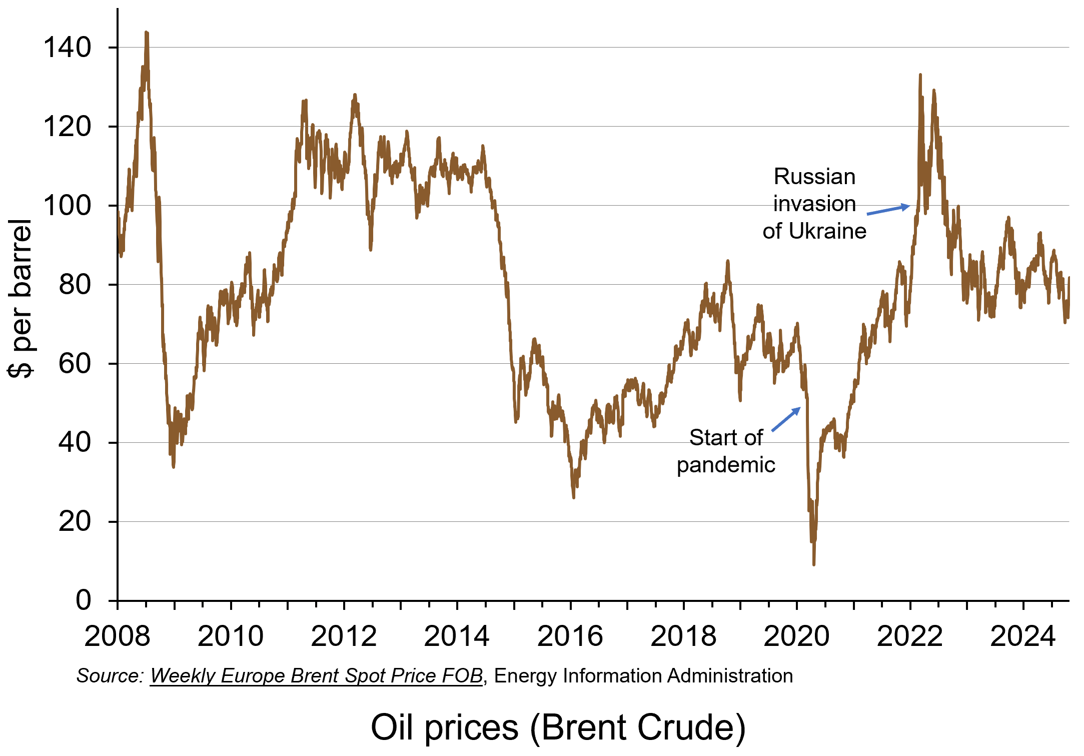 Over the past five years, global events have had a major impact on the price of oil. The economic conditions created by the impact of the COVID pandemic saw prices plummet from around $55 per barrel just before the pandemic in February 2020 to around $15 per barrel in April 2020. By mid-2021 they had recovered to around $75 per barrel. Then, in the aftermath of Russia’s invasion of Ukraine in February 2022, the price surged to reach $133 in June 2022. More recently, geopolitical tensions in the Middle East and concerns about China’s economic outlook have intensified concerns about the future direction of the market. (Click here for a PowerPoint of the chart.)
Geopolitical tensions
In the first week of October 2024, the price of crude oil rose by almost 10% to around $78 per barrel as the conflict in the Middle East intensified. It unfortunately comes at a time when many countries are starting to recover from the rise in oil prices caused by the pandemic and the war in Ukraine. Any increase in prices will affect the price that consumers pay to fill up their vehicles with fuel, just when prices of diesel and petrol had reached their lowest level for three years.
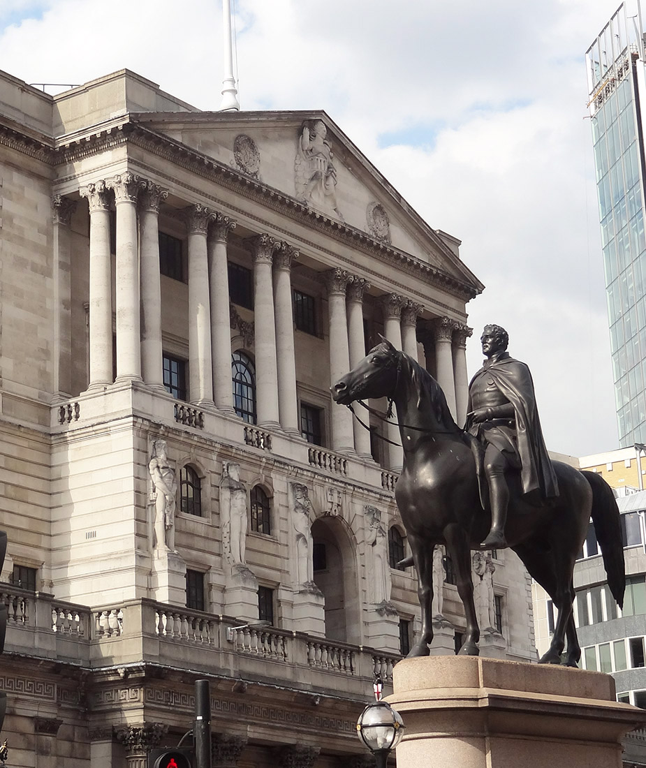 The Governor of the Bank of England, Andrew Bailey, has said that the Bank is monitoring developments in the Middle East ‘extremely closely’, as the conflict has the potential to have serious impacts in the UK. The Bank of England will therefore be watching for any movement in oil prices that could fuel inflation.
The main concerns stem from further escalation in the conflict between Israel and the Iran-backed armed group, Hezbollah, in Lebanon. If Israel decides to attack Iran’s oil sector, this is likely to cause a sharp rise in the price of oil. Iran is the world’s seventh largest oil exporter and exports over half of its production to China. If the oilfields of a medium-sized supplier, like Iran, were attacked, this could threaten general inflation in the UK, which could in turn influence any decision by the Bank of England to lower interest rates next month.
Supply deficits
This week (2nd week of October 2024) saw the price of crude oil surge above $81 per barrel to hit its highest level since August. This rise means that prices increased by 12% in a week. However, this surge in price also means that prices rose by almost 21% between the start September and the start of October alone. Yet it was only in early September when crude oil hit a year-to-date low, highlighting the volatility in the market.
As the Middle-East war enters a new and more energy-related phase, the loss of Iranian oil would leave the market in a supply deficit. The law of supply implies that such a deficit would lead to an increase in prices. This also comes at a time when the US Strategic Petroleum Reserve has also been depleted, causing further concerns about global oil supply.
 However, the biggest and most significant impact would be a disruption to flows through the Strait of Hormuz. This is a relatively narrow channel at the east end of the Persian Gulf through which a huge amount of oil tanker traffic passes – about a third of total seaborne-traded oil. It is therefore known as the world’s most important oil transit chokepoint. The risk that escalation could block the Strait of Hormuz could technically see a halt in about a fifth of the world’s oil supply. This would include exports from big Gulf producers, including Saudi Arabia, UAE, Kuwait and Iraq. In a worst-case scenario of a full closure of the Strait, a barrel of oil could very quickly rise to well above $100.
Disruption to shipments would also lead to higher gas prices and therefore lead to a rise in household gas and electricity bills. As with oil, gas prices filter down supply chains, affecting the cost of virtually all goods, resulting in a further rise in the cost of living. With energy bills in the UK having already risen by 10% for this winter, an escalation to the conflict could see prices rise further still.
China’s economic outlook

Despite the concern for the future supply of oil, there is also a need to consider how the demand for oil could impact price changes in the market. The price of oil declined on 14 October 2024 in light of concerns over China’s struggling economy. As China is the world’s largest importer of crude oil, there are emerging fears about the potential limits on fuel demand. This fall in price reversed increases made the previous week as investors become concerned about worsening deflationary pressures in China.
Any reduced demand from China could indicate an oversupply of crude oil and therefore potential price declines. Official data from China reveal a sharp year-on-year drop in the producer price index of 2.8% – the fastest decline in six months. These disappointing results have stirred uncertainty about the Chinese government’s economic stimulus plans. Prices could fall further if there are continuing doubts about the government’s ability to implement effective fiscal measures to promote consumer spending and, in turn, economic growth.
As a result of the 2% price fall in oil prices on 14 October, OPEC (the Organization of the Petroleum Exporting Countries) has lowered its 2024 and 2025 global oil demand growth. This negative news outweighed market concerns over the possibility that an Israeli response to Iran’s missile attack could disrupt oil production.
What is the future for oil prices?
 It is expected that the market for oil will remain a volatile one. Indeed, the current uncertainties around the globe only highlight this. It is never a simple task to predict what will happen in a market that is influenced by so many global factors, and the current global landscape only adds to the complexity.
There’s a wide spectrum of predictions about what could come next in the market for crude oil. Given the changes in the first two weeks of October alone, supply and demand factors from separate parts of the globe have made the future of oil prices particularly uncertain. Callum Macpherson, head of commodities at Investec, stated in early October that ‘there is really no way of telling where we will be this time next week’ (see the first BBC News article linked below).
Despite the predominately negative outlook, this is all based on potential scenarios. Caroline Bain, chief commodities economist at Capital Economics suggests that if the ‘worst-case scenario’ of further escalation in the Middle East conflict does not materialise, oil prices are likely to ‘ease back quite quickly’. Even if Iran’s supplies were disrupted, China could turn to Russia for its oil. Bain says that there is ‘more than enough capacity’ globally to cover the gap if Iranian production is lost. However, this does then raise the question of where the loyalty of Saudi Arabia, the world’s second largest oil producer, lies and whether it will increase or restrict further production.
What is certain is that the market for crude oil will continue to be a market that is closely observed. It doesn’t take much change in global activity for prices to move. Therefore, in the current political and macroeconomic environment, the coming weeks and months will be critical in determining oil prices and, in turn, their economic effects.
Articles
- How worried should I be about rising oil prices?
BBC News, Michael Race (4/10/24)
- Interest rates could fall more quickly, hints Bank
BBC News, Dearbail Jordan (3/10/24)
- Oil Prices Eye $100 A Barrel As War Risk Premium Returns
FX Empire, Phil Carr (8/10/24)
- Crude oil futures reverse previous gains following disappointing economic data from China
London Loves Business, Hamza Zraimek (14/10/24)
- Oil falls 2% as OPEC cuts oil demand growth view, China concerns
Reuters, Arathy Somasekhar (14/10/24)
- Could war in the Gulf push oil to $100 a barrel?
The Economist (7/10/24)
- The Commodities Feed: Oil remains volatile
ING Think, Ewa Manthey and Warren Patterson (8/10/24)
- Who and what is driving oil price volatility
FT Alphaville, George Steer (9/10/24)
- Brent crude surges above $80 as conflict and storm spark supply fears
Financial Times, Rafe Uddin and Jamie Smyth (7/10/24)
Questions
- Use a demand and supply diagram to illustrate what has happened to oil prices in the main two scenarios:
(a) Conflict in the Middle East;
(b) Concerns about China’s economic performance.
- How are the price elasticities of demand and supply relevant to the size of any oil price change?
- What policy options do the governments have to deal with the potential of increasing energy prices?
- What are oil futures? What determines oil future prices?
- How does speculation affect oil prices?
 We continue to live through incredibly turbulent times. In the past decade or so we have experienced a global financial crisis, a global health emergency, seen the UK’s departure from the European Union, and witnessed increasing levels of geopolitical tension and conflict. Add to this the effects from the climate emergency and it easy to see why the issue of economic uncertainty is so important when thinking about a country’s economic prospects.
In this blog we consider how we can capture this uncertainty through a World Uncertainty Index and the ways by which economic uncertainty impacts on the macroeconomic environment.
World Uncertainty Index
Hites Ahir, Nicholas Bloom and Davide Furceri have constructed a measure of uncertainty known as the World Uncertainty Index (WUI). This tracks uncertainty around the world using the process of ‘text mining’ the country reports produced by the Economist Intelligence Unit. The words searched for are ‘uncertain’, ‘uncertainty’ and ‘uncertainties’ and a tally is recorded based on the number of times they occur per 1000 words of text. To produce the index this figure is then multiplied up by 100 000. A higher number therefore indicates a greater level of uncertainty. For more information on the construction of the index see the 2022 article by Ahir, Bloom and Furceri linked below.
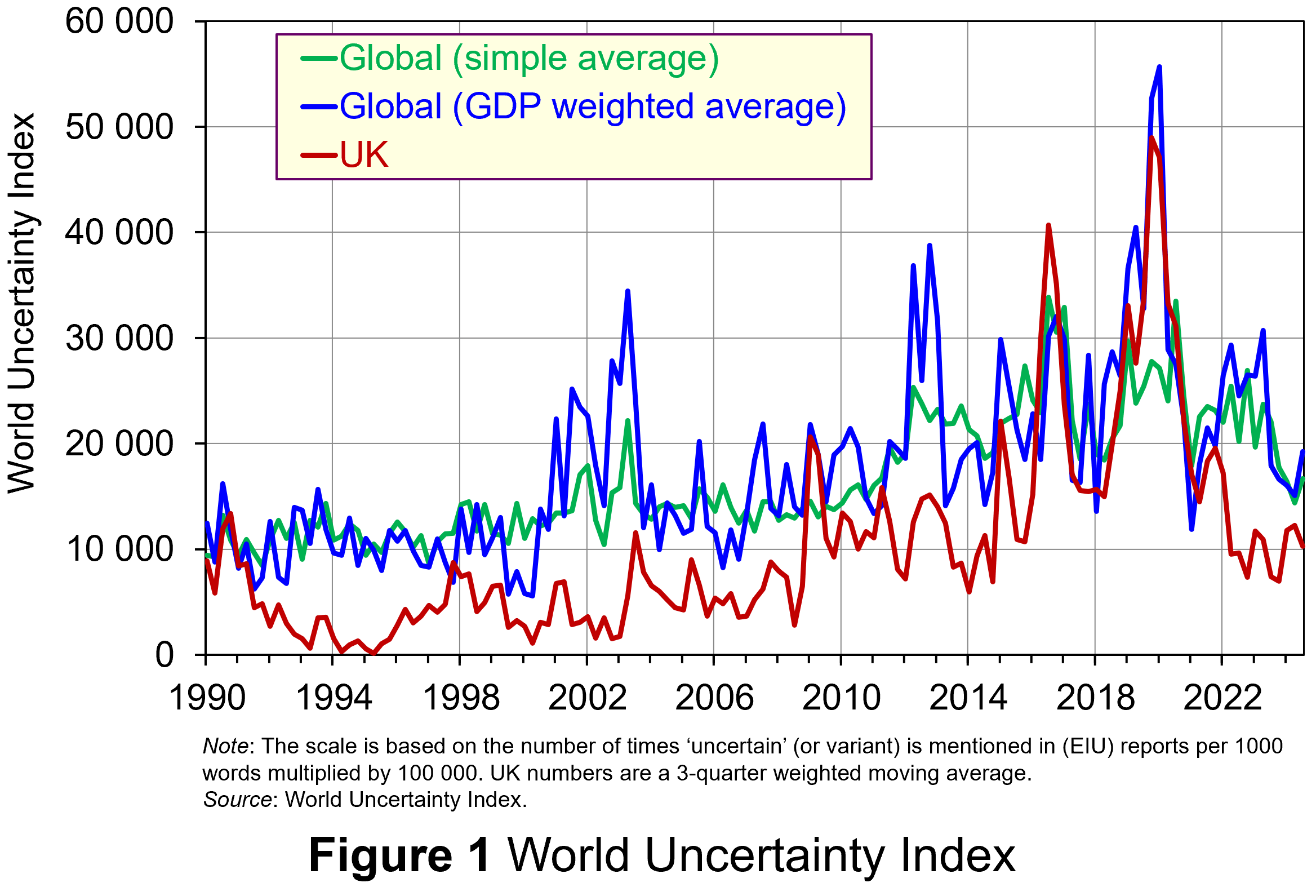 Figure 1 (click here for a PowerPoint) shows the WUI both globally and in the UK quarterly since 1991. The global index covers 143 countries and is presented as both a simple average and a GDP weighted average. The UK WUI is also shown. This is a three-quarter weighted average, the authors’ preferred measure for individual countries, where increasing weights of 0.1, 0.3 and 0.6 are used for the three most recent quarters.
From Figure 1 we can see how the level of uncertainty has been particularly volatile over the past decade or more. Events such as the sovereign debt crisis in parts of Europe in the early 2010s, the Brexit referendum in 2016, the COVID-pandemic in 2020–21 and the invasion of Ukraine in 2022 all played their part in affecting uncertainty domestically and internationally.
Uncertainty, risk-aversion and aggregate demand
Now the question turns to how uncertainty affects economies. One way of addressing this is to think about ways in which uncertainty affects the choices that people and businesses make. In doing so, we could think about the impact of uncertainty on components of aggregate demand, such as household consumption and investment, or capital expenditures by firms.
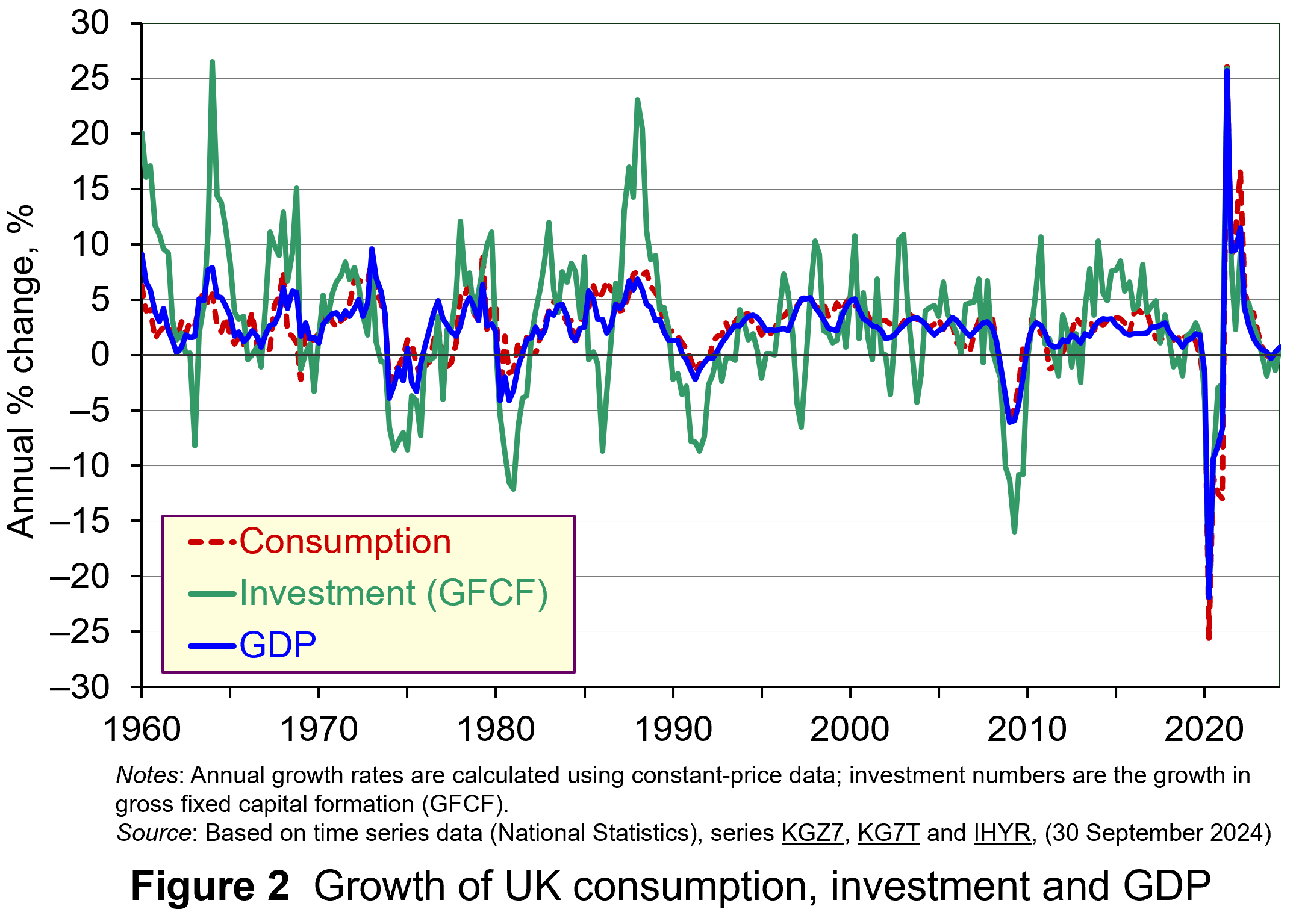 As Figure 2 shows (click here for a PowerPoint), investment is particularly volatile, and much more so than household spending. Some of this can be attributed to the ‘lumpiness’ of investment decisions since these expenditures tend to be characterised by indivisibility and irreversibility. This means that they are often relatively costly to finance and are ‘all or nothing’ decisions. In the context of uncertainty, it can make sense therefore for firms to wait for news that makes the future clearer. In this sense, we can think of uncertainty rather like a fog that firms are peering through. The thicker the fog, the more uncertain the future and the more cautious firms are likely to be.
The greater caution that many firms are likely to adopt in more uncertain times is consistent with the property of risk-aversion that we often attribute to a range of economic agents. When applied to household spending decisions, risk-aversion is often used to explain why households are willing to hold a buffer stock of savings to self-insure against unforeseen events and their future financial outcomes being worse than expected. Hence, in more uncertain times households are likely to want to increase this buffer further.
 The theory of buffer-stock saving was popularised by Christopher Carroll in 1992 (see link below). It implies that in the presence of uncertainty, people are prepared to consume less today in order to increase levels of saving, pay off existing debts, or borrow less relative to that in the absence of uncertainty. The extent of the buffer of financial wealth that people want to hold will depend on their own appetite for risk, the level of uncertainty, and the moderating effect from their own impatience and, hence, present bias for consuming today.
Risk aversion is consistent with the property of diminishing marginal utility of income or consumption. In other words, as people’s total spending volumes increase, their levels of utility or satisfaction increase but at an increasingly slower rate. It is this which explains why individuals are willing to engage with the financial system to reallocate their expected life-time earnings and have a smoother consumption profile than would otherwise be the case from their fluctuating incomes.
Yet diminishing marginal utility not only explains consumption smoothing, but also why people are willing to engage with the financial system to have financial buffers as self-insurance. It explains why people save more or borrow less today than suggested by our base-line consumption smoothing model. It is the result of people’s greater dislike (and loss of utility) from their financial affairs being worse than expected than their like (and additional utility) from them being better than expected. This tendency is only likely to increase the more uncertain times are. The result is that uncertainty tends to lower household consumption with perhaps ‘big-ticket items’, such as cars, furniture, and expensive electronic goods, being particularly sensitive to uncertainty.
Uncertainty and confidence
Uncertainty does not just affect risk; it also affects confidence. Risk and confidence are often considered together, not least because their effects in generating and transmitting shocks can be difficult to disentangle.
We can think of confidence as capturing our mood or sentiment, particularly with respect to future economic developments. Figure 3 plots the Uncertainty Index for the UK alongside the OECD’s composite consumer and business confidence indicators. Values above 100 for the confidence indicators indicate greater confidence about the future economic situation and near-term business environment, while values below 100 indicate pessimism towards the future economic and business environments.
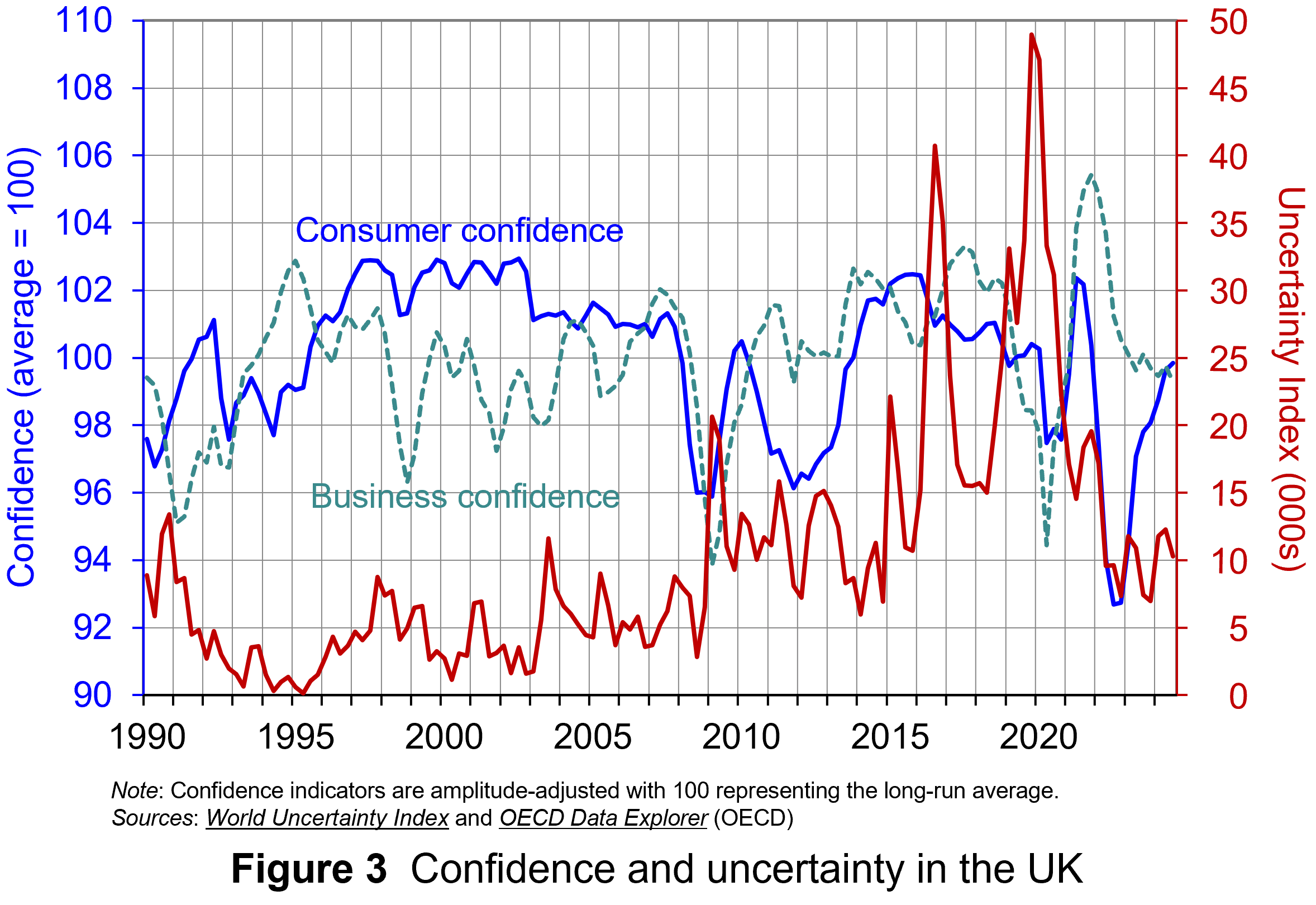 Figure 3 suggests that the relationship between confidence and uncertainty is rather more complex than perhaps is generally understood (click here for a PowerPoint). Haddow, Hare, Hooley and Shakir (see link below) argue that the evidence tends to point to changes in uncertainty affecting confidence, but with less evidence that changes in confidence affect uncertainty.
To illustrate this, consider the global financial crisis of the late 2000s. The argument can be made that the heightened uncertainty about future prospects for households and businesses helped to erode their confidence in the future. The result was that people and businesses revised down their expectations of the future (pessimism). However, although people were more pessimistic about the future, this was more likely to have been the result of uncertainty rather than the cause of further uncertainty.
Conclusion
For economists and policymakers alike, indicators of uncertainty, such as the Ahir, Bloom and Furceri World Uncertainty Index, are invaluable tools in understanding and forecasting behaviour and the likely economic outcomes that follow. Some uncertainty is inevitable, but the persistence of greater uncertainty since the global financial crisis of the late 2000s compares quite starkly with the relatively lower and more stable levels of uncertainty seen from the mid-1990s up to the crisis. Hence the recent frequency and size of changes in uncertainty show how important it to understand how uncertainty effects transmit through economies.
Academic papers
- The World Uncertainty Index
National Bureau of Economic Research, Working Paper 29763, Hites Ahir, Nicholas Bloom and Davide Furceri (February 2022)
- The Buffer-Stock Theory of Saving: Some Macroeconomic Evidence
Brookings Papers on Economic Activity, Christopher D Carroll (Vol 2, 1992)
- Macroeconomic uncertainty: what is it, how can we measure it and why does it matter?
Bank of England Quarterly Bulletin, 2013 Q2, Abigail Haddow, Chris Hare, John Hooley and Tamarah Shakir (13/6/13)
Articles
Data
Questions
- (a) Explain what is meant by the concept of diminishing marginal utility of consumption.
(b) Explain how this concept helps us to understand both consumption smoothing and the motivation to engage in buffer-stock saving.
- Explain the distinction between confidence and uncertainty when analysing macroeconomic shocks.
- Discuss which types of expenditures you think are likely to be most susceptible to uncertainty shocks.
- Discuss how economic uncertainty might affect productivity and the growth of potential output.
- How might the interconnectedness of economies affect the transmission of uncertainty effects through economies?
 When I worked as a professional economist at HM Treasury and later the Council of Mortgage Lenders (now part of UK Finance), I would regularly brief on the state of the affordability of housing, with a particular focus on the owner-occupied market. That was back in the late 1990s. Fast forward a quarter of a century and I recognise not only how much I have aged but also how deep-rooted and long-standing the affordability problem is.
It is perhaps not surprising that in her first speech as the new Chancellor of the Exchequer, Rachel Reeves, referenced directly the housing market and the need to address supply-side issues. She has set a target of one and a half million new homes built over the next five years.
It is therefore timely to revisit the trends in house prices across the UK. By applying the distinction between nominal and real values we get a very clear sense of the deteriorating affordability of housing.
Nominal house price patterns
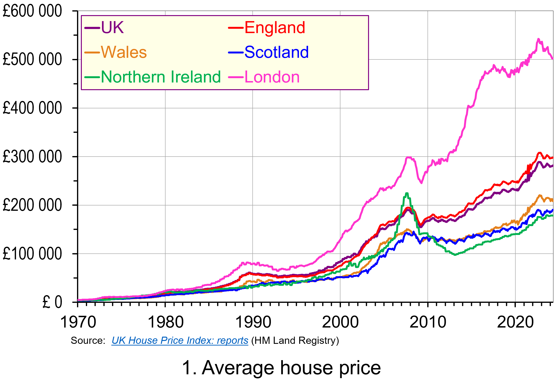 The average UK actual or nominal house price in April 2024 was £281 000. As Chart 1 shows, this masks considerable differences across the UK. In England the average price was £298 000 (105 per cent of the UK average), though this is heavily skewed by London where the average price was £502 000 (178 per cent of the UK average). Meanwhile, in Scotland it was £190 000 (68 per cent of the UK average), in Wales £208 000 (74 per cent of the UK average) and in Northern Ireland it was £178 000 (74 per cent of the UK average). (Click here to download a PowerPoint copy of the chart.)
A simple comparison of the average house price in April 2024 with January 1970 reveals a 72-fold increase in the UK, an 80-fold increase in England, including a 101-fold increase in London, a 65-fold increase in Wales, a 59-fold increase in Scotland and a 45-fold increase in Northern Ireland. Whilst these figures are sensitive to the particular period over which we choose to measure, there is little doubting that upward long-term trend in house prices.
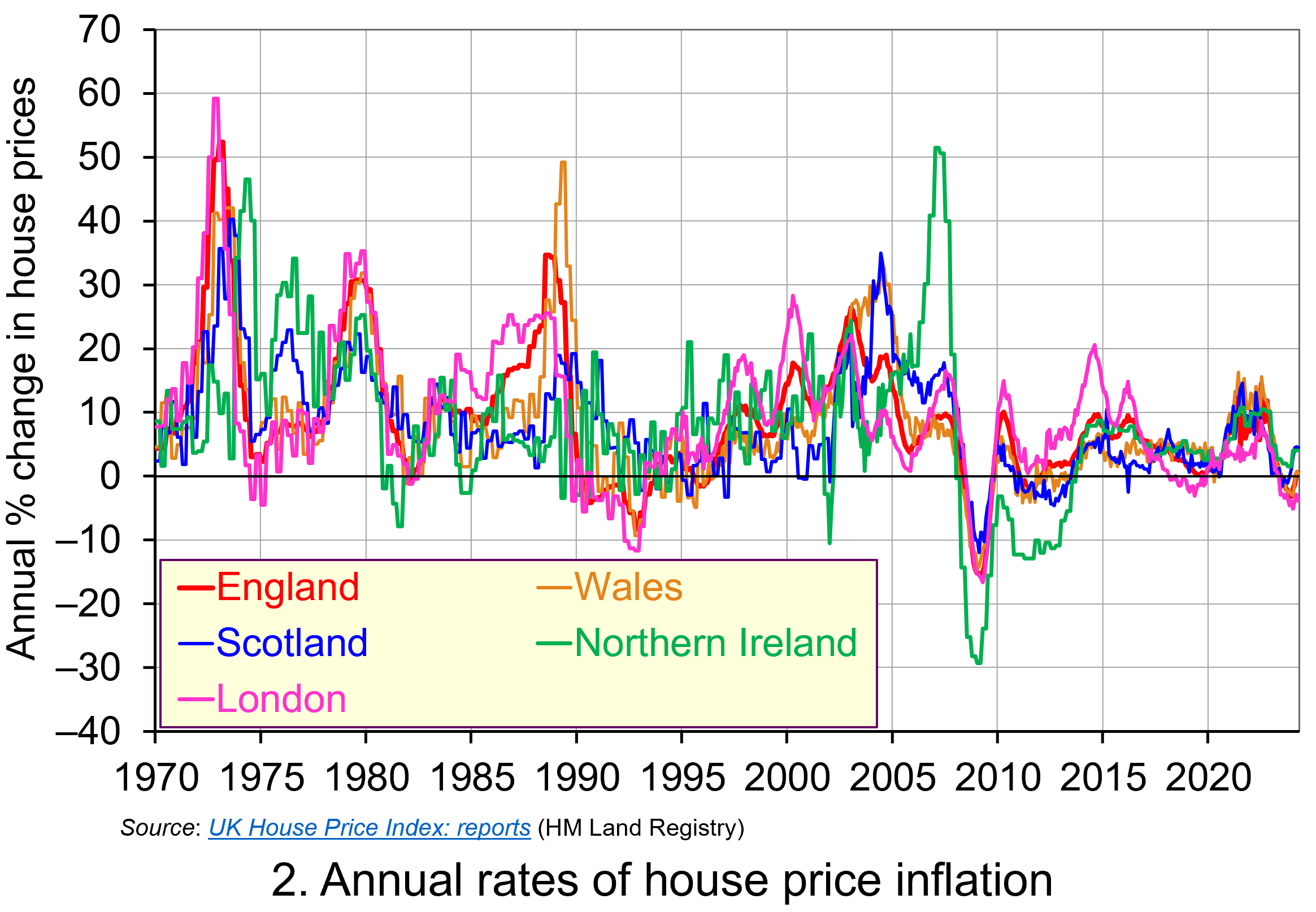 Whilst nominal prices trend upwards over time, the short-term rates of increase are highly volatile. This can be seen from an inspection of Chart 2, which shows the annual rates of increase across the four nations of the UK, as well as for London. This is evidence of frequent imbalances between the flows of property on to the market to sell (instructions to sell) and the number of people looking to buy (instructions to buy). An increase in instructions to buy (housing demand) relative to those to sell (housing supply) puts upward pressure on prices; an increase in the number of instructions to sell (housing supply) relative to those to buy (housing demand) puts downward pressure on prices. (Click here to download a PowerPoint copy of the chart.)
Chart 2 nicely captures the recent slowdown in the housing market. The inflationary shock that began to take hold in 2021 led the Bank of England to raise Bank Rate on 15 occasions – from 0.25 per cent in December 2021 to 5.25 per cent in August 2023 (which remains the rate at the time of writing, but could be cut at the next Bank of England meeting on 1 August 2024). Higher Bank Rate has pushed up mortgage rates, which has contributed to an easing of housing demand. Demand has also been dampened by weak growth in the economy, higher costs of living and fragile consumer confidence. The result has been a sharp fall in the rate of house price inflation, with many parts of the UK experiencing house price deflation. As the chart shows, the rate of deflation has been particularly pronounced and protracted in London, with house prices in January 2024 falling at an annual rate of 5.1 per cent.
Real house price patterns
Despite the volatility in house prices, such as those of recent times, the longer-term trend in house prices is nonetheless upwards. To understand just how rapidly UK house prices have grown over time, we now consider their growth relative to consumer prices. This allows us to analyse the degree to which there has been an increase in real house prices.
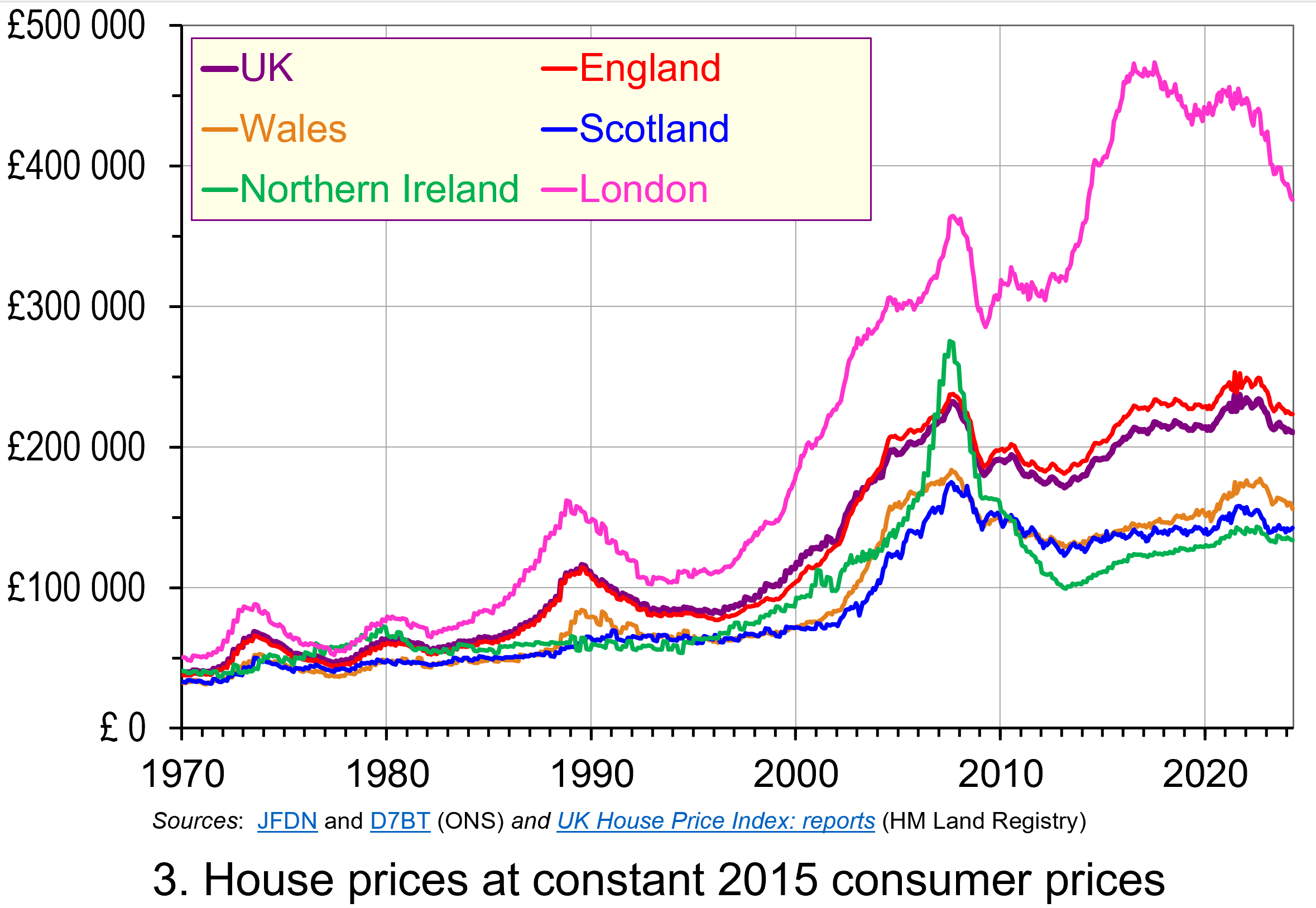 To calculate real or inflation-adjusted house prices, we deflate nominal house prices by the Consumer Prices Index (CPI). Chart 3 shows the resulting real house prices series across the UK as if consumer prices were fixed at 2015 levels.
The key message here is that over the longer-term we cannot fully explain the growth in actual (nominal) house prices by the growth in consumer prices. Rather, we see real increases in house prices. Inflation-adjusted UK house prices were 5.3 times higher in April 2024 compared to January 1970. For England the figure was 5.9 times, Wales 4.8 times, Scotland 4.3 times and for Northern Ireland 3.3 times. In London, inflation-adjusted house prices were 7.4 times higher. (Click here to download a PowerPoint copy of the chart.)
As we saw with nominal house prices, the estimated long-term increase in real house prices is naturally sensitive to the period over which we measure. For example, the average real UK house price in August 2022 was 5.8 times higher than in January 1970, while in London they were 8.7 times higher. But the message is clear – the long-term increase is not merely nominal, reflecting increasing prices generally, but is real, reflecting pressures that are increasing house prices relative to general price levels.
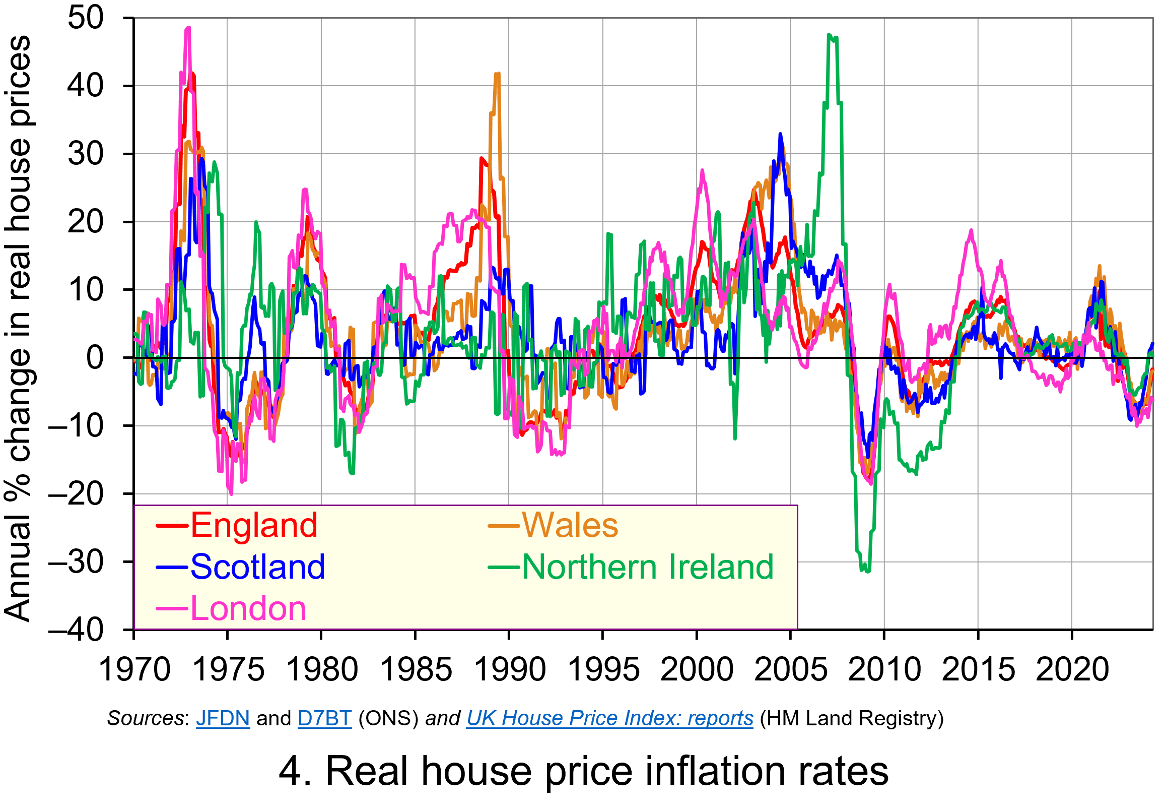 Chart 4 shows how the volatility in house prices continues to be evident when house prices are adjusted for changes in consumer prices. The UK’s annual rate of real house price inflation was as high as 40 per in January 1973; on the other hand, in June 1975 inflation-adjusted house prices were 15 per cent lower than a year earlier. (Click here to download a PowerPoint copy of the chart.)
Over the period from January 1970 to April 2024, the average annual rate of real house price inflation in the UK was 3.2 per cent. Hence house prices have, on average, grown at an annual rate of consumer price inflation plus 3.2 per cent. For the four nations, real house price inflation has averaged 3.8 per cent in England, 3.4 per cent in Wales, 3.0 per cent in Scotland and 2.9 per cent in Northern Ireland. Further, the average rate of real house price inflation in London since January 1970 has been 4.5 per cent. By contrast, that for the East and West Midlands has been 3.7 and 3.5 per cent respectively. The important point here is that the pace with which inflation-adjusted house prices have risen helps to contextualise the extent of the problem of housing affordability – a problem that only worsens over time when real incomes do not keep pace.
House building
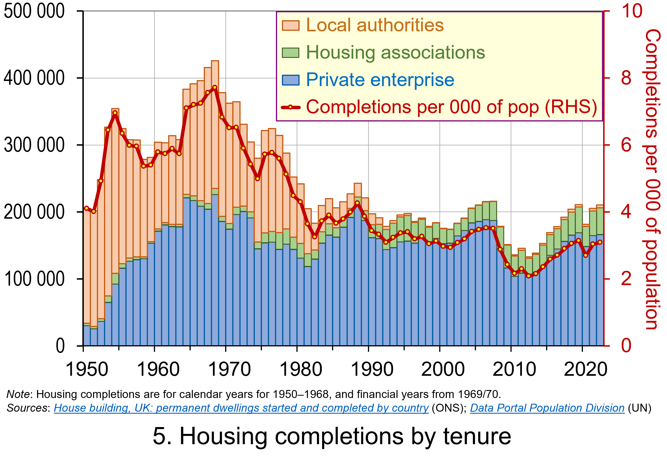 The newly elected Labour government has made the argument that it needs to prioritise planning reform as an engine for economic growth. While this ambition extends beyond housing, the scale of the supply-side problem facing the housing market can be seen in Chart 5. The chart shows the number of housing completions in the UK since 1950 by type of tenure. (Click here to download a PowerPoint copy of the chart.)
The chart shows the extent of the growth in house building in the UK that occurred from the 1950s and into the 1970s. Over these three decades the typical number of new properties completed each year was around 320 000 or 6 per thousand of the population. The peak of house building was in the late 1960s when completions exceeded 400 000 per year or over 7.5 per thousand of the population. It is also noticeable how new local authority housing (‘council houses’) played a much larger role in the overall housing mix.
Since 1980, the average number of housing completions each year has dropped to 191 000 or 3.2 per thousand of the population. If we consider the period since 2000, the number of completions has averaged only 181 000 per year or 2.9 per thousand of the population. While it is important to understand the pressures on housing demand in any assessment of the growth in real house prices, the lack of growth in supply is also a key factor. The fact that less than half the number of properties per thousand people are now being built compared with half a century or so ago is an incredibly stark statistic. It is a major determinant of the deterioration of housing affordability.
However, there are important considerations around the protection of the natural environment that need to be considered too. It will therefore be interesting to see how the reforms to planning develop and what their impact will be on house prices and their affordability.
Articles
- Rachel Reeves requests urgent assessment of spending inheritance
The Guardian, Larry Elliott (8/7/24)
- Reeves to bring back housebuilding targets
BBC News, Faisal Islam and Daniel Thomas (8/7/24)
- UK Chancellor Reeves Vows to Fix Broken Planning System for Housebuilding
Bloomberg UK, Tom Rees, Damian Shepherd, and Joe Mayes (8/7/24)
- What to expect for house prices for the rest of 2024
i News, Callum Mason (10/7/24)
- UK house prices still unaffordable for many people, says Nationwide
The Guardian, Richard Partington (1/7/24)
- House prices still unaffordable for the average earner despite wage rises – Nationwide
Sky News, Sarah Taaffe-Maguire (1/7/24)
- Labour cannot build 1.5m homes without cash for affordable housing, providers say
The Guardian, Jack Simpson (12/7/24)
Statistics
Questions
- Explain the difference between a rise in the rate of house price inflation a rise in the level of house prices.
- Explain the difference between nominal and real house prices.
- If nominal house prices rise can real house price fall? Explain your answer.
- What do you understand by the terms instructions to buy and instructions to sell?
- What factors are likely to affect the levels of instructions to buy and instructions to sell?
- How does the balance between instructions to buy and instructions to sell affect house prices?
- How can we differentiate between different housing markets? Illustrate your answer with examples.
- What metrics could be used to measure the affordability of housing?
- Discuss the argument that the deterioration of housing affordability is the result of market failure.
 On 25 October 2024, Moody’s, one of the major credit ratings agencies, announced that it was downgrading France’s economic outlook to negative. This was its first downgrading of France since 2012. It followed a similar revision by Fitch’s, another ratings agency, on 11 October.
 The yield on 10-year French government debt began 2024 at 2.56% and had an upward trend for the first half of the year. The yield peaked at 3.34% on 1 July. It then fell back below 3% for a while. The negative economic outlook then pushed yields back above 3% and they finished October at 3.12%, half a percentage point above the level at the start of the year. This represents a significant increase in borrowing costs for the French government.
 If the expected rate of return rises, this increases the discount rate applied to future cash flows and reduces their present value. At the current price, the fixed coupon is not sufficient to compensate investors. So, investors sell the bonds and price falls until it reaches a point where the yield offered is equal to that required. The reverse happens if the expected rate of return falls.
  Governments in France last achieved a balanced budget in 1974. They have run deficits ever since. Figure 2 illustrates the French government budget deficits from 1990 to 2023 (click here for a PowerPoint). The figure shows that France experienced deficits in the past similar to today’s. These, however, did not tend to worry bond markets too much.
 Further, political instability has grown due to the inconclusive parliamentary elections which Emmanuel Macron surprisingly called in July. No single political grouping has a majority and the President has appointed a Centrist Prime Minister, Michel Barnier (the former EU Brexit negotiator). His government is trying to pass a budget through the Assemblée Nationale involving a mixture of spending cuts and tax hikes which amount to savings of €60 billion ($66 billion). This is equivalent to 2% of GDP.
 In the past, bond investors were more tolerant of France’s budget deficits. French government bonds were attractive options for investors wanting to hold euro-denominated bonds while avoiding riskier Southern European countries such as Greece, Italy, Portugal and Spain. Since France has run persistent government deficits for a long time, it offered bond investors a more liquid market than more fiscally-parsimonious Northern European neighbours, such as Germany and the Netherlands. Consequently, France’s debt instruments offered a slight risk premium on the yields for those countries.
  As Figure 3 illustrates, this was the culmination of a trend evident throughout 2024, with the difference in yields between the two declining steadily (click here for a PowerPoint). At the start of the year, the yield on Spanish debt offered a 40 basis points premium over the French equivalent. By October, the yield on Spanish debt was consistently below that of French debt. All of this is due to bond investors’ rising expectations about France’s credit default risk. Now, France’s borrowing costs are not only above Spain, but also closer to those of Greece and Italy than of Germany.
  The UK government announced on 14 October 2024 in a ministerial statement that it intended to raise the threshold for the ring-fencing (separation) of retail and investment banking activities of large UK-based banks. These banks are known as ‘systemically important financial institutions (SIFIs)’, which are currently defined as those with more than £25bn of core retail deposits. Under the new regulations, the threshold would rise from £25bn to £35bn.
 Ring-fencing was recommended by the Independent Commission on Banking (ICB) in 2011 (see link below) and implemented through the Financial Services (Banking Reform) Act of 2013. The proposed separation of core retail banking services from investment banking were intended to address issues in banks which arose during the global financial crisis and which required substantial taxpayer bailouts. (See the 2011 blog,
  When that market crashed in 2007, several UK-based banks incurred significant losses, as did other banks around the world. Given their thin equity buffers and the inability to borrow due to a credit crunch, such banks found it impossible to bear these losses.
 It must be noted that most of the criticism comes from banks themselves. They state that it required significant operational restructuring by UK banks subject to the regulatory framework which was complex and costly.
 One of the most famous Acts of Congress relating to finance and financial markets in the USA is the Glass-Steagall Act of 1933. The Act was passed in the aftermath of the 1929 Wall Street crash and the onset of the Great Depression in the USA. That witnessed significant bank failures across the country and problems were traced back to significant losses made by banks in their lending to investors during the speculative frenzy that preceded the stock market crash of 1929.
 The market for crude oil is usually a volatile one. Indeed, in the last few months, the market has seen prices rise and fall due to various supply and demand influences. Crude oil is coined the ‘King of Commodities’ due to the impact it has on consumers, producers and both the micro and macro economy. The price of crude oil affects everything from the cost of producing plastics, transportation, and food at the supermarket.
 Over the past five years, global events have had a major impact on the price of oil. The economic conditions created by the impact of the COVID pandemic saw prices plummet from around $55 per barrel just before the pandemic in February 2020 to around $15 per barrel in April 2020. By mid-2021 they had recovered to around $75 per barrel. Then, in the aftermath of Russia’s invasion of Ukraine in February 2022, the price surged to reach $133 in June 2022. More recently, geopolitical tensions in the Middle East and concerns about China’s economic outlook have intensified concerns about the future direction of the market. (Click
  The Governor of the Bank of England, Andrew Bailey, has said that the Bank is monitoring developments in the Middle East ‘extremely closely’, as the conflict has the potential to have serious impacts in the UK. The Bank of England will therefore be watching for any movement in oil prices that could fuel inflation.
 However, the biggest and most significant impact would be a disruption to flows through the Strait of Hormuz. This is a relatively narrow channel at the east end of the Persian Gulf through which a huge amount of oil tanker traffic passes – about a third of total seaborne-traded oil. It is therefore known as the world’s most important oil transit chokepoint. The risk that escalation could block the Strait of Hormuz could technically see a halt in about a fifth of the world’s oil supply. This would include exports from big Gulf producers, including Saudi Arabia, UAE, Kuwait and Iraq. In a worst-case scenario of a full closure of the Strait, a barrel of oil could very quickly rise to well above $100.
 It is expected that the market for oil will remain a volatile one. Indeed, the current uncertainties around the globe only highlight this. It is never a simple task to predict what will happen in a market that is influenced by so many global factors, and the current global landscape only adds to the complexity.
 We continue to live through incredibly turbulent times. In the past decade or so we have experienced a global financial crisis, a global health emergency, seen the UK’s departure from the European Union, and witnessed increasing levels of geopolitical tension and conflict. Add to this the effects from the climate emergency and it easy to see why the issue of economic uncertainty is so important when thinking about a country’s economic prospects.
 Figure 1 (click
  As Figure 2 shows (click
  The theory of buffer-stock saving was popularised by Christopher Carroll in 1992 (see link below). It implies that in the presence of uncertainty, people are prepared to consume less today in order to increase levels of saving, pay off existing debts, or borrow less relative to that in the absence of uncertainty. The extent of the buffer of financial wealth that people want to hold will depend on their own appetite for risk, the level of uncertainty, and the moderating effect from their own impatience and, hence, present bias for consuming today.
 Figure 3 suggests that the relationship between confidence and uncertainty is rather more complex than perhaps is generally understood (click
  When I worked as a professional economist at
  The average UK actual or nominal house price in April 2024 was £281 000. As Chart 1 shows, this masks considerable differences across the UK. In England the average price was £298 000 (105 per cent of the UK average), though this is heavily skewed by London where the average price was £502 000 (178 per cent of the UK average). Meanwhile, in Scotland it was £190 000 (68 per cent of the UK average), in Wales £208 000 (74 per cent of the UK average) and in Northern Ireland it was £178 000 (74 per cent of the UK average). (Click
  Whilst nominal prices trend upwards over time, the short-term rates of increase are highly volatile. This can be seen from an inspection of Chart 2, which shows the annual rates of increase across the four nations of the UK, as well as for London. This is evidence of frequent imbalances between the flows of property on to the market to sell (instructions to sell) and the number of people looking to buy (instructions to buy). An increase in instructions to buy (housing demand) relative to those to sell (housing supply) puts upward pressure on prices; an increase in the number of instructions to sell (housing supply) relative to those to buy (housing demand) puts downward pressure on prices. (Click
  To calculate real or inflation-adjusted house prices, we deflate nominal house prices by the Consumer Prices Index (CPI). Chart 3 shows the resulting real house prices series across the UK as if consumer prices were fixed at 2015 levels.
 Chart 4 shows how the volatility in house prices continues to be evident when house prices are adjusted for changes in consumer prices. The UK’s annual rate of real house price inflation was as high as 40 per in January 1973; on the other hand, in June 1975 inflation-adjusted house prices were 15 per cent lower than a year earlier. (Click
  The newly elected Labour government has made the argument that it needs to prioritise planning reform as an engine for economic growth. While this ambition extends beyond housing, the scale of the supply-side problem facing the housing market can be seen in Chart 5. The chart shows the number of housing completions in the UK since 1950 by type of tenure. (Click