 In recent months there has been growing uncertainty across the global economy as to whether the US economy was going to experience a ‘hard’ or ‘soft landing’ in the current business cycle – the repeated sequences of expansion and contraction in economic activity over time. Announcements of macroeconomic indicators have been keenly anticipated for signals about how quickly the US economy is slowing.
Such heightened uncertainty is a common feature of late-cycle slowing economies, but uncertainty now has been exacerbated because it has been a while since developed economies have experienced a business cycle like the current one. The 21st century has been characterised by low inflation, low interest rates and recessions caused by various types of crises – a stock market crisis (2001), a banking crisis (2008) and a global pandemic (2020). In contrast, the current cycle is a throwback to the 20th century. The high inflation and the ensuing increases in interest rates have produced a business cycle which echoes the 1970s. Therefore, few investors have experience of such economic conditions.
The focus for investors during this stage of the cycle is when the slowing economy will reach the minimum. They will also be concerned with the depth of the slowdown: will there still be some growth in income, albeit low; or will the trough be severe enough to produce a recession, and, if so, how deep? Given uncertainty around the length and magnitude of business cycles, this leads to greater risk aversion among investors. This affects reactions to announcements of leading and lagging macroeconomic indicators.
This blog examines what sort of economic conditions we should expect in a late-cycle economy. It analyses the impact this has had on investor behaviour and the ensuing dynamics observed in financial markets in the USA.
The Business Cycle

The business cycle refers to repeated sequences of expansion and contraction (or slowdown) in economic activity over time. Figure 1 illustrates a typical cycle. Typically, these sequences include four main stages. In each one there are different effects on consumer and business confidence:
- Expansion: During this stage, the economy experiences growth in GDP, with incomes and consumption spending rising. Business and consumer confidence are high. Unemployment is falling.
- Peak: This is the point at which the economy reaches its maximum output, but growth has ceased (or slowed). At this stage, inflationary pressures peak as the economy presses against potential output. This tends to result in tighter monetary policy (higher interest rates).
- Slowdown: The higher interest rates raise the cost of borrowing and reduce consumption and investment spending. Consumption and incomes both slow or fall. (Figure 1 illustrates the severe case of falling GDP (negative growth) in this stage.) Unemployment starts rising.
- Trough: This is the lowest point of the cycle, where economic activity bottoms out and the economy begins to recover. This can be associated with slow but still rising national income (a soft landing) or national income that has fallen (a hard landing, as shown in Figure 1).
While business cycles are common enough to enable such characterisation of their temporal pattern, their length and magnitude are variable and this produces great uncertainty, particularly when cycles approach peaks and troughs.
 As an economy’s cycle approaches a trough, such as US economy’s over the past few months, uncertainty is exacerbated. The high interest rates used to tackle inflation will have increased borrowing costs for businesses and consumers. Access to credit may have become more restricted. Profit margins are reduced, especially for industrial sectors sensitive to the business cycle, reducing expected cash flows.
The combination of these factors can increase the risk of a recession, producing greater volatility in financial markets. This manifests itself in increased risk aversion among investors.
Utility theory suggests that, in general, investors will exhibit loss aversion. This means that they do not like bearing risk, fearing that the return from an investment may be less than expected. In such circumstances, investors need to be compensated for bearing risk. This is normally expressed in terms of expected financial return. To bear more risk, investors require higher levels of return as compensation.
As perceptions of risk change through the business cycle, so this will change the return investors will require from the financial instruments they hold. Perceived higher risk raises the return investors will require as compensation. Conversely, lower perceived risk decreases the return investors expect as compensation.
Investors’ expected rate of return is manifested in the discount rate that they use to value the anticipated cash flows from financial instruments in discounted cash flow (DCF) analysis. Equation 1 is the algebraic expression of the present-value discounted series of cash flows for financial instruments:

Where:
V = present value
C = anticipated cash flows in each of time periods 1, 2, 3, etc.
r = expected rate of return
For fixed-income debt securities, the cash flow is constant, while for equity securities (shares), expectations regarding cash flows can change.
Slowing economies and risk aversion
 In a slowing economy, with great uncertainty about the scale and timing of the bottom of the cycle, investors become more risk averse about the prospects of firms. This this leads to higher risk premia for financial instruments sensitive to a slowdown in economic activity.
This translates into a higher expected return and higher discount rate used in the valuation of these instruments (r in equation 1). This produces decreases in perceived value, decreased demand and decreased prices for these financial instruments. This can be observed in the market dynamics for these instruments.
First, there may be a ‘flight to safety’. Investors attach a higher risk premium to risker financial instruments, such as equities, and seek a ‘safe-haven’ for their wealth. Therefore, we should observe a reorientation from more risky to less risky assets. Demand for equities falls, while demand for safer assets, such as government bonds and gold, rises.
There is some evidence for this behaviour as uncertainty about the US economic outlook has increased. Gold, long seen as a hedge against market decline, is at record highs. US Government bond prices have risen too.
To analyse whether this may be a flight to safety, I analysed the correlation between the daily US government bond price (5-year Treasury Bill) and share prices represented by the two more significant stock market indices in the USA: the S&P 500 and the Nasdaq Composite. I did this for two different time periods. Table 1 shows the results. Panel (a) shows the correlation coefficients for the period between 1 May 2024 and 31 July 2024; Panel (b) shows the correlation coefficients for the period between 1 August 2024 and 9 September 2024.

In the period between May and July 2024, the 5-year Treasury Bill and share price indices had significantly positive correlations. When share prices rose, the Treasury Bill’s price rose; when share prices fell, the bill’s price fell. During that period, expectations about falling interest rates dominated valuations and that effected the valuations of all financial instruments in the same way – lower expected interest rates reduce the opportunity cost of holding instruments and reduces the expected rates of return. Hence, the discount rate applied to cash flows is reduced, and present value rises. The opposite happens when macroeconomic indicators suggest that interest rates will stay high (ceteris paribus).
As the summer proceeded, worries about a ‘hard landing’ began to concern investors. A weak jobs report in early August particularly exercised markets, producing a ‘flight to safety’. Greater risk aversion among investors meant that they expect a higher return from equities. This reduced perceived value, reducing demand and price (ceteris paribus). To insulate themselves from higher risk, investors bought safer assets, like government bonds, thereby pushing up their prices. This behaviour was consistent with the significant negative correlation observed between US government debt prices and the S&P 500 and Nasdaq indices in Panel (b).
Another signal of increased risk aversion among investors is ‘sector rotation’ in their equity portfolios. Increased risk aversion among investors will lead them to divest from ‘cyclical’ companies. Such companies are in industrial sectors which are more sensitive to the changing economic conditions across the business cycle – consumer discretionary and communication services sectors, for example. To reduce their exposure to risk, investors will switch to ‘defensive’ sectors – those less sensitive to the business cycle. Examples include consumer staples and utility sectors.
Cyclical sectors will suffer a greater adverse impact on their cash flows and risk in a slowing economy. Consequently, investors expect higher return as compensation. This reduces the value of those shares. Demand for them falls, depressing their price. In contrast, defensive sectors will be valued more. They will see an increase in demand and price. This sector rotation seems to have happened in August (2024). Figure 2 shows the percentage change between 1 August and 9 September 2024 in the S&P 500 index and four sector indices, comprising companies from the communication services, consumer discretionary, consumer staples and utilities sectors.

Overall, the S&P 500 index was slightly higher, as shown by the first bar in the chart. However, while the cyclical sectors experienced decreases in their share prices, particularly communication services, the defensive companies experienced large price increases – nearly 3% for utilities and over 6% for consumer staples.
Conclusion
Economies experience repeated sequences of expansion and contraction in economic activity over time. At the moment, the US economy is approaching the end of its current slowing phase. Increased uncertainty is a common feature of late-cycle economies and this manifests itself in heightened risk aversion among investors. This produces certain dynamics which have been observable in US debt and equity markets. This includes a ‘flight to safety’, with investors divesting risky financial instruments in favour of safer ones, such as US government debt securities and gold. Also, investors have been reorientating their equity portfolios away from cyclicals and towards defensive securities.
Articles
- America’s recession signals are flashing red. Don’t believe them
The Economist (22/8/24)
- The most well-known recession indicator stopped flashing red, but now another one is going off
CNN, Elisabeth Buchwald (13/9/24)
- World’s largest economy will still achieve soft landing despite rising unemployment, most analysts believe
Financial Times, Claire Jones, Delphine Strauss and Martha Muir (6/8/24)
- We’re officially on slowdown watch
Financial Times, Robert Armstrong and Aiden Reiter (30/8/24)
- Anatomy of a rout
Financial Times, Robert Armstrong and Aiden Reiter (6/8/24)
- Reasons why investors need to prepare for a US recession
Financial Times, Peter Berezin (5/9/24)
- Business Cycle: What It Is, How to Measure It, and Its 4 Phases
Investopedia, Lakshman Achuthan (6/6/24)
- Risk Averse: What It Means, Investment Choices, and Strategies
Investopedia, James Chen (5/8/24)
Data
Questions
- What is risk aversion? Sketch an indifference curve for a risk-averse investor, treating expected return and risk as two-characteristics of a financial instrument.
- Show what happens to the slope of the indifference curve if the investor becomes more risk averse.
- Using demand and supply analysis, illustrate and explain the impact of a flight to safety on the market for (i) company shares and (ii) US government Treasury Bills.
- Use economic theory to explain why the consumer discretionary sector may be more sensitive than the consumer staples sector to varying incomes across the economic cycle.
- Research the point of the economic cycle that the US economy has reached as you read this blog. What is the relationship between bond and equity prices? Which sectors have performed best in the stock market?
 The past decade or so has seen large-scale economic turbulence. As we saw in the blog Fiscal impulses, governments have responded with large fiscal interventions. The COVID-19 pandemic, for example, led to a positive fiscal impulse in the UK in 2020, as measured by the change in the structural primary balance, of over 12 per cent of national income.
The scale of these interventions has led to a significant increase in the public-sector debt-to-GDP ratio in many countries. The recent interest rates hikes arising from central banks responding to inflationary pressures have put additional pressure on the financial well-being of governments, not least on the financing of their debt. Here we discuss these pressures in the context of the ‘r – g’ rule of sustainable public debt.
Public-sector debt and borrowing
 Chart 1 shows the path of UK public-sector net debt and net borrowing, as percentages of GDP, since 1990. Debt is a stock concept and is the result of accumulated flows of past borrowing. Net debt is simply gross debt less liquid financial assets, which mainly consist of foreign exchange reserves and cash deposits. Net borrowing is the headline measure of the sector’s deficit and is based on when expenditures and receipts (largely taxation) are recorded rather than when cash is actually paid or received. (Click here for a PowerPoint of Chart 1)
Chart 1 shows the impact of the fiscal interventions associated with the global financial crisis and the COVID-19 pandemic, when net borrowing rose to 10 per cent and 15 per cent of GDP respectively. The former contributed to the debt-to-GDP ratio rising from 35.6 per cent in 2007/8 to 81.6 per cent in 2014/15, while the pandemic and subsequent cost-of-living interventions contributed to the ratio rising from 85.2 per cent in 2019/20 to around 98 per cent in 2023/24.
Sustainability of the public finances
") The ratcheting up of debt levels affects debt servicing costs and hence the budgetary position of government. Yet the recent increases in interest rates also raise the costs faced by governments in financing future deficits or refinancing existing debts that are due to mature. In addition, a continuation of the low economic growth that has beset the UK economy since the global financial crisis also has implications for the burden imposed on the public sector by its debts, and hence the sustainability of the public finances. After all, low growth has implications for spending commitments, and, of course, the flow of receipts.
The ratcheting up of debt levels affects debt servicing costs and hence the budgetary position of government. Yet the recent increases in interest rates also raise the costs faced by governments in financing future deficits or refinancing existing debts that are due to mature. In addition, a continuation of the low economic growth that has beset the UK economy since the global financial crisis also has implications for the burden imposed on the public sector by its debts, and hence the sustainability of the public finances. After all, low growth has implications for spending commitments, and, of course, the flow of receipts.
The analysis therefore implies that the sustainability of public-sector debt is dependent on at least three factors: existing debt levels, the implied average interest rate facing the public sector on its debts, and the rate of economic growth. These three factors turn out to underpin a well-known rule relating to the fiscal arithmetic of public-sector debt. The rule is sometimes known as the ‘r – g’ rule (i.e. the interest rate minus the growth rate).
Underpinning the fiscal arithmetic that determines the path of public-sector debt is the concept of the ‘primary balance’. This is the difference between the sector’s receipts and its expenditures less its debt interest payments. A primary surplus (a positive primary balance) means that receipts exceed expenditures less debt interest payments, whereas a primary deficit (a negative primary balance) means that receipts fall short. The fiscal arithmetic necessary to prevent the debt-to-GDP ratio rising produces the following stable debt equation or ‘r – g’ rule:
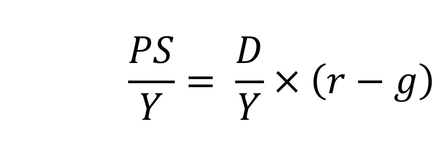
On the left-hand side of the stable debt equation is the required primary surplus (PS) to GDP (Y) ratio. Moving to the right-hand side, the first term is the existing debt-to-GDP ratio (D/Y). The second term ‘r – g’, is the differential between the average implied interest rate the government pays on its debt and the growth rate of the economy. These terms can be expressed in either nominal or real terms as this does not affect the differential.
To illustrate the rule consider a country whose existing debt-to-GDP ratio is 1 (i.e. 100 per cent) and the ‘r – g’ differential is 0.02 (2 percentage points). In this scenario they would need to run a primary surplus to GDP ratio of 0.02 (i.e. 2 percent of GDP).
The ‘r – g‘ differential
The ‘r – g’ differential reflects macroeconomic and financial conditions. The fiscal arithmetic shows that these are important for the dynamics of public-sector debt. The fiscal arithmetic is straightforward when r = g as any primary deficit will cause the debt-to-GDP ratio to rise, while a primary surplus will cause the ratio to fall. The larger is g relative to r the more favourable are the conditions for the path of debt. Importantly, if the differential is negative (r < g), it is possible for the public sector to run a primary deficit, up to the amount that the stable debt equation permits.
 Consider Charts 2 and 3 to understand how the ‘r – g’ differential has affected debt sustainability in the UK since 1990. Chart 2 plots the implied yield on 10-year government bonds, alongside the annual rate of nominal growth (click here for a PowerPoint). As John explains in his blog The bond roller coaster, the yield is calculated as the coupon rate that would have to be paid for the market price of a bond to equal its face value. Over the period, the average annual nominal growth rate was 4.5 per cent, while the implied interest rate was almost identical at 4.6 per cent. The average annual rate of CPI inflation over this period was 2.8 per cent.
 Chart 3 plots the ‘r – g’ differential which is simply the difference between the two series in Chart 2, along with a 12-month rolling average of the differential to help show better the direction of the differential by smoothing out some of the short-term volatility (click here for a PowerPoint). The differential across the period is a mere 0.1 percentage points implying that macroeconomic and financial conditions have typically been neutral in supporting debt sustainability. However, this does mask some significant changes across the period.
We observe a general downward trend in the ‘r – g’ differential from 1990 up to the time of the global financial crisis. Indeed between 2003 and 2007 we observe a favourable negative differential which helps to support the sustainability of public debt and therefore the well-being of the public finances. This downward trend of the ‘r – g’ differential was interrupted by the financial crisis, driven by a significant contraction in economic activity. This led to a positive spike in the differential of over 7 percentage points.
 Yet the negative differential resumed in 2010 and continued up to the pandemic. Again, this is indicative of the macroeconomic and financial environments being supportive of the public finances. It was, however, largely driven by low interest rates rather than by economic growth.
Consequently, the negative ‘r – g’ differential meant that the public sector could continue to run primary deficits during the 2010s, despite the now much higher debt-to-GDP ratio. Yet, weak growth was placing limits on this. Chart 4 indeed shows that primary deficits fell across the decade (click here for a PowerPoint).
The pandemic and beyond
 The pandemic saw the ‘r – g’ differential again turn markedly positive, averaging 7 percentage points in the four quarters from Q2 of 2020. While the differential again turned negative, the debt-to-GDP ratio had also increased substantially because of large-scale fiscal interventions. This made the negative differential even more important for the sustainability of the public finances. The question is how long the negative differential can last.
Looking forward, the fiscal arithmetic is indeed uncertain and worryingly is likely to be less favourable. Interest rates have risen and, although inflationary pressures may be easing somewhat, interest rates are likely to remain much higher than during the past decade. Geopolitical tensions and global fragmentation pose future inflationary concerns and a further drag on growth.
As well as the short-term concerns over growth, there remain long-standing issues of low productivity which must be tackled if the growth of the UK economy’s potential output is to be raised. These concerns all point to the important ‘r – g’ differential become increasingly less negative, if not positive. If so the fiscal arithmetic could mean increasingly hard maths for policymakers.
Articles
- The budget deficit: a short guide
House of Commons Library (8/6/23)
- If markets are right about long real rates, public debt ratios will increase for some time. We must make sure that they do not explode.
Peterson Institute for International Economics, Olivier Blanchard (6/11/23)
- The UK government’s debt nightmare
ITV News, Robert Peston (13/7/23)
- National debt could hit 300% of GDP by 2070s, independent watchdog the OBR warns
Sky News, James Sillars (13/7/23)
- How much money is the UK government borrowing, and does it matter?
BBC News (20/10/23)
- Cost of national debt hits 20-year high
BBC News, Vishala Sri-Pathma & Faisal Islam (4/10/23)
- Bond markets could see ‘mini boom-bust cycles’ as global government debt to soar by $5 trillion a yea
Markets Insider, Filip De Mott (16/11/23)
- The counterintuitive truth about deficits for bond investors
Financial Times, Matt King (17/11/23)
- UK government borrowing almost £20bn lower than expected
The Guardian, Richard Partington (20/10/23)
- Controlling debt is just a means — it is not a government’s end
Financial Times, Martin Wolf (13/11/23)
Data
Questions
- What is meant by each of the following terms: (a) net borrowing; (b) primary deficit; (c) net debt?
- Explain how the following affect the path of the public-sector debt-to-GDP ratio: (a) interest rates; (b) economic growth; (c) the existing debt-to-GDP ratio.
- Which factors during the 2010s were affecting the fiscal arithmetic of public debt positively, and which negatively?
- Discuss the prospects for the fiscal arithmetic of public debt in the coming years.
- Assume that a country has an existing public-sector debt-to-GDP ratio of 60 percent.
(a) Using the ‘rule of thumb’ for public debt dynamics, calculate the approximate primary balance it would need to run in the coming year if the expected average real interest rate on the debt were 3 per cent and real economic growth were 2 per cent?
(b) Repeat (a) but now assume that real economic growth is expected to be 4 per cent.
(c) Repeat (a) but now assume that the existing public-sector debt-to-GDP ratio is 120 per cent.
(d) Using your results from (a) to (c) discuss the factors that affect the fiscal arithmetic of the growth of public-sector debt.
 To finance budget deficits, governments have to borrow. They can borrow short-term by issuing Treasury bills, typically for 1, 3 or 6 months. These do not earn interest and hence are sold at a discount below the face value. The rate of discount depends on supply and demand and will reflect short-term market rates of interest. Alternatively, governments can borrow long-term by issuing bonds. In the UK, these government securities are known as ‘gilts’ or ‘gilt-edged securities’. In the USA they are known as ‘treasury bonds’, ‘T-bonds’ or simply ‘treasuries’. In the EU, countries separately issue bonds but the European Commission also issues bonds.
In the UK, gilts are issued by the Debt Management Office on behalf of the Treasury. Although there are index-linked gilts, the largest proportion of gilts are conventional gilts. These pay a fixed sum of money per annum per £100 of face value. This is known as the ‘coupon payment’ and the rate is set at the time of issue. The ‘coupon rate’ is the payment per annum as a percentage of the bond’s face value:

Payments are made six-monthly. Each issue also has a maturity date, at which point the bonds will be redeemed at face value. For example, a 4½% Treasury Gilt 2028 bond has a coupon rate of 4½% and thus pays £4.50 per annum (£2.25 every six months) for each £100 of face value. The issue will be redeemed in June 2028 at face value. The issue was made in June 2023 and thus represented a 5-year bond. Gilts are issued for varying lengths of time from 2 to 55 years. At present, there are 61 different conventional issues of bonds, with maturity dates varying from January 2024 to October 2073.
Bond prices
 Bonds can be sold on the secondary market (i.e. the stock market) before maturity. The market price, however, is unlikely to be the coupon price (i.e. the face value). The lower the coupon rate relative to current interest rates, the less valuable the bond will be. For example, if interest rates rise, and hence new bonds pay a higher coupon rate, the market price of existing bonds paying a lower coupon rate must fall. Thus bond prices vary inversely with interest rates.
The market price also depends on how close the bonds are to maturity. The closer the maturity date, the closer the market price of the bond will be to the face value.
Bond yields: current yield
A bond’s yield is the percentage return that a person buying the bond receives. If a newly issued bond is bought at the coupon price, its yield is the coupon rate.
However, if an existing bond is bought on the secondary market (the stock market), the yield must reflect the coupon payments relative to the purchase price, not the coupon price. We can distinguish between the ‘current yield’ and the ‘yield to maturity’.
The current yield is the coupon payment as a percentage of the current market price of the bond:

Assume a bond were originally issued at 2% (its coupon rate) and thus pays £2 per annum. In the meantime, however, assume that interest rates have risen and new bonds now have a coupon rate of 4%, paying £4 per annum for each £100 invested. To persuade people to buy old bonds with a coupon rate of 2%, their market prices must fall below their face value (their coupon price). If their price halved, then they would pay £2 for every £50 of their market price and hence their current yield would be 4% (£2/£50 × 100).
Bond yields: yield to maturity (YTM)
But the current yield does not give the true yield – it is only an approximation. The true yield must take into account not just the market price but also the maturity value and the length of time to maturity (and the frequency of payments too, which we will ignore here). The closer a bond is to its maturity date, the higher/lower will be the true yield if the price is below/above the coupon price: in other words, the closer will the market price be to the coupon price for any given market rate of interest.
A more accurate measure of a bond’s yield is thus the ‘yield to maturity’ (YTM). This is the interest rate which makes the present value of all a bond’s future cash flows equal to its current price. These cash flows include all coupon payments and the payment of the face value on maturity. But future cash flows must be discounted to take into account the fact that money received in the future is worth less than money received now, since money received now could then earn interest.
The yield to maturity is the internal rate of return (IRR) of the bond. This is the discount rate which makes the present value (PV) of all the bond’s future cash flows (including the maturity payment of the coupon price) equal to its current market price. For simplicity, we assume that coupon payments are made annually. The formula is the one where the bond’s current market price is given by:

Where: t is the year; n is the number of years to maturity; YTM is the yield to maturity.
Thus if a bond paid £5 each year and had a maturity value of £100 and if current interest rates were higher than 5%, giving a yield to maturity of 8%, then the bond price would be:

In other words, with a coupon rate of 5% and a higher YTM of 8%, the bond with a face value of £100 and five years to maturity would be worth only £88.02 today.
If you know the market price of a given bond, you can work out its YTM by substituting in the above formula. The following table gives examples.

The higher the YTM, the lower the market price of a bond. Since the YTM reflects in part current rates of interest, so the higher the rate of interest, the lower the market price of any given bond. Thus bond yields vary directly with interest rates and bond prices vary inversely. You can see this clearly from the table. You can also see that market bond prices converge on the face value as the maturity date approaches.
Recent activity in bond markets
Investing in government bonds is regarded as very safe. Coupon payments are guaranteed, as is repayment of the face value on the maturity date. For this reason, many pension funds hold a lot of government bonds issued by financially trustworthy governments. But in recent months, bond prices in the secondary market have fallen substantially as interest rates have risen. For those holding existing bonds, this means that their value has fallen. For governments wishing to borrow by issuing new bonds, the cost has risen as they have to offer a higher coupon rate to attract buyers. This make it more expensive to finance government debt.
 The chart shows the yield on 10-year government bonds. It is calculated using the ‘par value’ approach. This gives the coupon rate that would have to be paid for the market price of a bond to equal its face value. Clearly, as interest rates rise, a bond would have to pay a higher coupon rate for this to happen. (This, of course, is only hypothetical to give an estimate of market rates, as coupon rates are fixed at the time of a bond’s issue.)
Par values reflect both yield to maturity and also expectations of future interest rates. The higher people expect future interest rates to be, the higher must par values be to reflect this.
 In the years following the financial crisis of 2007–8 and the subsequent recession, and again during the COVID pandemic, central banks cut interest rates and supported this by quantitative easing. This involved central banks buying existing bonds on the secondary market and paying for them with newly created (electronic) money. This drove up bond prices and drove down yields (as the chart shows). This helped support the policy of low interest rates. This was a boon to governments, which were able to borrow cheaply.
This has all changed. With quantitative tightening replacing quantitative easing, central banks have been engaging in asset sales, thereby driving down bond prices and driving up yields. Again, this can be seen in the chart. This has helped to support a policy of higher interest rates.
Problems of higher bond yields/lower bond prices
Although lower bond prices and higher yields have supported a tighter monetary policy, which has been used to fight inflation, this has created problems.
First, it has increased the cost of financing government debt. In 2007/8, UK public-sector net debt was £567bn (35.6% of GDP). The Office for Budget Responsibility forecasts that it will be £2702bn (103.1% of GDP in the current financial year – 2023/24). Not only, therefore, are coupon rates higher for new government borrowing, but the level of borrowing is now a much higher proportion of GDP. In 2020/21, central government debt interest payments were 1.2% of GDP; by 2022/23, they were 4.4% (excluding interest on gilts held in the Bank of England, under the Asset Purchase Facility (quantitative easing)).
 In the USA, there have been similar increases in government debt and debt interest payments. Debt has increased from $9tn in 2007 to $33.6tn today. Again, with higher interest rates, debt interest as a percentage of GDP has risen: from 1.5% of GDP in 2021 to a forecast 2.5% in 2023 and 3% in 2024. What is more, 31 per cent of US government bonds will mature next year and will need refinancing – at higher coupon rates.
There is a similar picture in other developed countries. Clearly, higher interest payments leave less government revenue for other purposes, such as health and education.
Second, many pension funds, banks and other investment companies hold large quantities of bonds. As their price falls, so this reduces the value of these companies’ assets and makes it harder to finance new purchases, or payments or loans to customers. However, the fact that new bonds pay higher interest rates means that when existing bond holdings mature, the money can be reinvested at higher rates.
Third, bonds are often used by companies as collateral against which to borrow and invest in new capital. As bond prices fall, this can hamper companies’ ability to invest, which will lead to lower economic growth.
Fourth, higher bond yields divert demand away from equities (shares). With equity markets falling back or at best ceasing to rise, this erodes the value of savings in equities and may make it harder for firms to finance investment through new issues.
At the core of all these problems is inflation and budget deficits. Central banks have responded by raising interest rates. This drives up bond yields and drives down bond prices. But bond prices and yields depend not just on current interest rates, but also on expectations about future interest rates. Expectations currently are that budget deficits will be slow to fall as governments seek to support their economies post-COVID. Also expectations are that inflation, even though it is falling, is not falling as fast as originally expected – a problem that could be exacerbated if global tensions increase as a result of the ongoing war in Ukraine, the Israel/Gaza war and possible increased tensions with China concerning disputes in the China Sea and over Taiwan. Greater risks drive up bond yields as investors demand a higher interest premium.
Articles
Information and data
Questions
- Why do bond prices and bond yields vary inversely?
- How are bond yields and prices affected by expectations?
- Why are ‘current yield’ and ‘yield to maturity’ different?
- What is likely to happen to bond prices and yields in the coming months? Explain your reasoning.
- What constraints do bond markets place on fiscal policy?
- Would it be desirable for central banks to pause their policy of quantitative tightening?
 March 2023 saw the failure of Silicon Valley Bank (SVB), a regional US bank based in California that focused on financial services for the technology sector. It also saw the forced purchase of global-banking giant, Credit Suisse, by rival Swiss bank, UBS. These events fuelled concerns over the banking sector’s financial well-being, with fears for other financial institutions and the wider economy.
Yet it is not the only sector where concerns abound over financial well-being. The cost-of-living crisis, the hike in interest rates and the economic slowdown continue to have an adverse impact on the finances of households and businesses. Furthermore, many governments face difficult fiscal choices in light of the effects of recent economic shocks, such as COVID and the Russian invasion of Ukraine, on the public finances.
Balance sheets and flow accounts
When thinking about the financial well-being of people, business and governments it is now commonplace for economists to reference balance sheets. This may seem strange to some since it is easy to think of balance sheets as the domain of accountants or those working in finance. Yet balance sheets, and the various accounts that lie behind them, are essential in analysing financial well-being and, therefore, in helping to understand economic behaviour and outcomes. Hence, it is important for economists to embrace them too.
 A balance sheet is a record of stocks of assets and liabilities of individuals or organisations. Behind these stocks are accounts capturing flows, including income, expenditure, saving and borrowing. There are three types of flow accounts: income, financial and capital. Together, the balance sheets and flow accounts provide important insights into the overall financial position of individuals or organisations as well as the factors contributing to changes in their financial well-being.
The stock value of a sector’s or country’s non-financial assets and its net financial worth (i.e. the balance of financial assets over liabilities) is referred to as its net worth. Non-financial assets include produced assets, such as dwellings and other buildings, machinery and computer software, and non-produced assets, largely land.
An increase in the net worth of the sectors or the whole country implies greater financial well-being, while a decrease implies greater financial stress. Yet a deeper understanding of financial well-being also requires an analysis of the composition of the balance sheets as well as their potential vulnerabilities from shocks, such as interest rate rises, falling asset prices or borrowing constraints.
UK net worth
 The chart shows the UK’s stock of net worth since 1995, alongside its value relative to annual national income (GDP) (click here for a PowerPoint). In 2021, the net worth of the UK was £11.8 trillion, equivalent to 5.2 times the country’s annual GDP. This marked an increase of £1.0 trillion or 9 per cent over 2020. This was driven largely by an increase in land values (non-produced non-financial assets).
In contrast, the stock of net worth fell in both 2008 and 2009 at the height of the financial crisis and the ensuing economic slowdown, which contributed to the country’s net worth falling by over 8 per cent.
The chart shows that net financial assets continue to make a negative contribution to the country’s net worth. In 2021 financial liabilities exceeded financial assets by the equivalent of 19 per cent of annual national income.
Non-financial corporations and the public sector together had financial liabilities in excess of financial assets of £3.4 trillion and £2.5 trillion respectively. However, once non-financial assets are accounted for, non-financial corporations had a positive net worth of £607 billion, although their value was not sufficient to prevent the public sector having a negative net worth of £1.2 trillion. Meanwhile, households had a positive net worth of £11.4 trillion and financial corporations a negative net worth of £4.9 billion.
Vulnerabilities and the balance sheets
The collapse of Silicon Valley Bank (SVB) resulted from balance sheet distress. Some argue that this distress can be attributed to a mismanagement of the bank’s liquidity position, which saw the bank use the surge in funds, on the back of buoyant activity among technology companies, to purchase long-dated bonds while, at the same time, reducing the share of assets held in cash. However, as the growth of the technology sector slowed as pandemic restrictions eased and, crucially, as central banks, including the Federal Reserve, began raising rates, the value of these long-dated bonds fell. This is because there is a negative relationship between interest rates and bond prices. Bonds pay a fixed rate of interest and so as other interest rates rise, bonds become less attractive to savers, pushing down their price. As depositors withdrew funds, Silicon Valley Bank found itself increasingly trying to generate liquidity from assets whose value was falling.
A major problem with balance sheet distress is contagion. This can occur, in part, because of what is known as ‘counterparty risk’. This simply refers to the idea that one party’s well-being is tied directly to that of another. However, the effects on economies from counterparty risks can be amplified by their impact on general credit conditions, confidence and uncertainty. This helps to explain why the US government stepped in quickly to guarantee SVB deposits.
There is, however, a ‘moral hazard’ problem here: if central banks are always prepared to step in, it can signal to banks that they are too big to fail and disincentivise them for adopting appropriate risk management strategies in the first place.
Subsequently, First Citizens Bank acquired the commercial banking business of SVB, while its UK subsidiary was acquired by HSBC for £1.
Interest rates and financial well-being
In light of the failures of SVB and Credit Suisse, the raising of interest rates by inflation-targeting central banks has raised concerns about the liquidity and liabilities positions of banks and non-bank financial institutions, such as hedge funds, insurers and pension funds. As we have seen, higher interest rates push down the value of bonds, which form a major part of banks’ balance sheets. The problem for central banks is that, if this forced them to make large-scale injections of liquidity by buying bonds (quantitative easing), it would make the fight against inflation more difficult. Quantitative easing is the opposite of tightening monetary policy and thus credit conditions, which are seen as necessary to control inflation.
 Yet the raising of interest rates has implications for the financial well-being of other sectors too since they also are affected by the effects on asset values and debt-servicing costs. For example, raising interest rates has a severe impact on the cashflow of UK homeowners with large variable-rate mortgages. This can substantially affect their spending. The UK has a high proportion of homeowners on variable-rate mortgages or fairly short-term fixed-rate mortgages. Also for a large number of households their mortgages are high relative to their incomes.
In short, falling asset values and increasing debt-servicing costs from rising interest rates in response to rising inflation tends to dampen spending in the economy. The effects will be larger the more burdened with debt people and businesses are, and the less liquidity they have to access. This has the potential to lead to a financial consolidation in order to restore the well-being of balance sheets. This involves cutting borrowing and spending.
Such a consolidation could be exacerbated if financial institutions become distressed and if it were to result in even larger numbers of people and businesses facing greater restrictions in accessing credit. These balance sheet pressures will continue to weigh on the policy responses of central banks as they attempt to navigate economies out of the current inflationary pressures.
Articles
Questions
- What is recorded on a balance sheet? Explain with reference to the household sector.
- What is meant by net worth? Does an increase in net worth mean that an individual’s or sector’s financial well-being has increased?
- What is meant by ‘liquidity-constrained’ individuals or businesses? What factors might explain how liquidity constraints arise?
- It is sometimes argued that there is a predator-prey relationship between income and debt. How could such a relationship arise and what is its importance for the economy?
- Why might a deterioration of a country’s balance sheets have both national and international consequences?
- Explain the possible trade-offs facing central banks when responding to inflationary pressures.
 You may have been following the posts on the US debt ceiling and budget crisis: Over the cliff and Over the cliff: an update. Well, after considerable brinkmanship over the past couple of weeks, and with the government in partial shutdown since 1 October thanks to no budget being passed, a deal was finally agreed by both Houses of Congress, less than 12 hours before the deadline of 17 October. This is the date when the USA would have bumped up against the debt ceiling of $16.699 trillion and would be in default – unable to borrow sufficient funds to pay its bills, including maturing debt.
But the deal only delays the problem of a deeply divided Congress, with the Republican majority on the House of Representatives only willing to make a long-term agreement in exchange for concessions by President Obama and the Democrats on the healthcare reform legislation. All that has been agreed is to suspend the debt ceiling until 7 February 2014 and fund government until 15 January 2014.
A more permanent solution is clearly needed: not just one that raises the debt ceiling before the next deadline, but one which avoids such problems in the future. Such concerns were echoed by Christine Lagarde, Managing Director of the International Monetary Fund (IMF), who issued the following statement:
The U.S. Congress has taken an important and necessary step by ending the partial shutdown of the federal government and lifting the debt ceiling, which enables the government to continue its operations without disruption for the next few months while budget negotiations continue to unfold.
It will be essential to reduce uncertainty surrounding the conduct of fiscal policy by raising the debt limit in a more durable manner. We also continue to encourage the U.S. to approve a budget for 2014 and replace the sequester with gradually phased-in measures that would not harm the recovery, and to adopt a balanced and comprehensive medium-term fiscal plan.
US default: Congress votes to end shutdown crisis The Telegraph, Raf Sanchez (17/10/13)
US shutdown: Christine Lagarde calls for stability after debt crisis is averted The Guardian,
James Meikle, Paul Lewis and Dan Roberts (17/10/13)
America’s economy: Meh ceiling? The Economist (15/10/13)
Relief as US approves debt deal BBC News (17/10/13)
Shares in Europe dip after US debt deal BBC News (17/10/13)
Dollar slides as relief at U.S. debt deal fades Reuters, Richard Hubbard (17/10/13)
US debt deal: Analysts relieved rather than celebrating Financial Times, John Aglionby and Josh Noble (17/10/13)
Greenspan fears US government set for more debt stalemate BBC News (21/10/13)
Questions
- Explain what is meant by default and how the concept applies to the USA if it had not suspended or raised its budget ceiling.
- Is the agreement of October 16 likely to ‘reassure markets’? Explain your reasoning.
- What is likely to happen to long-term interest rates as a result of the agreement?
- Will the imposition of a new debt ceiling by February 2014 remove the possibility of using fiscal policy to stimulate aggregate demand and speed up the recovery?
- What is meant by ‘buy the rumour, sell the news’ in the context of stock markets? How was this relevant to the agreement on the US debt ceiling and budget?
