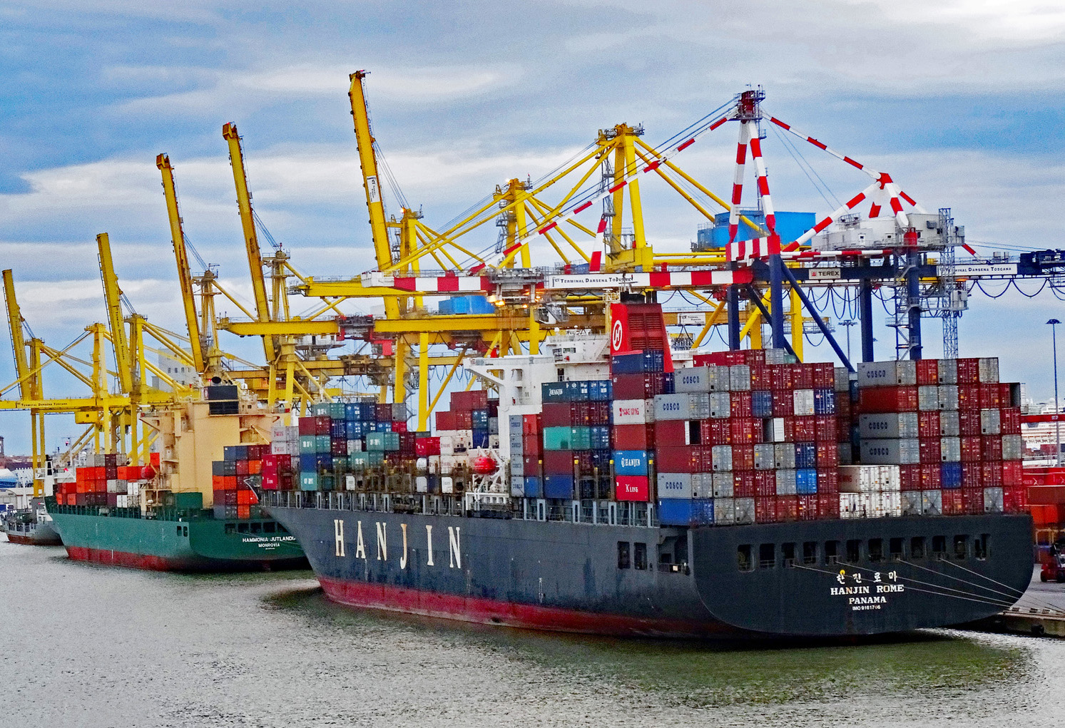
 The UK signed three trade deals in May – one with the USA, one with India and one with the EU. It is hoped by the government that these trade deals will provide a welcome boost to the UK economy.
The deal with the USA reduced tariffs on UK car exports to the USA from 27.5% to 10%, and on steel and aluminium exports from 25% to 0%. Pharmaceutical exports would also get more favourable treatment and there would be ‘reciprocal market access on beef’ (but with no lowering of food standards). Nevertheless, President Trump’s baseline tariff of 10% on most goods remains, as with other countries. However, a ruling by the US Court of International Trade has found that the Trump’s use of emergency powers to justify the sweeping use of tariffs is wrong. The Trump administration is appealing against the ruling and until the appeal is heard, the tariffs have been reinstated. Also, on May 30, the Trump administration announced that tariffs on steel and aluminium imports would rise from 25% to 50%. It remained to be seen whether this would affect the deal to reduce the rate to zero for British steel and aluminium imports.
The deal with India involves a reduction in tariffs on UK exports – some to zero – and simplified trade rules, faster customs clearance, less paperwork and the freedom for UK businesses to provide telecommunications and construction services. In return, tariffs will be reduced to zero on 99% of Indian exports to the UK. The UK government estimates that deal will result in trade between the two countries increasing by over 30%, with the UK’s GDP expanding by around 0.1 percentage points per year.
UK-EU trade
 Perhaps the most significant new trade deal, however, is with the EU. This is a major advance on the current post-Brexit Trade and Cooperation Agreement (TCA). Under the TCA, there are no tariffs or quotas on UK goods exports to the EU or EU goods exports to the UK. However, to ensure that it is EU and UK business that benefits from these ‘trade preferences’, firms must show that their products fulfil ‘rules of origin’ requirements.
Under rules of origin requirements, when a good is imported into the UK from outside the EU and then has value added to it by processing, packaging, cleaning, remixing, preserving, refashioning, etc., it can only count as a UK good if sufficient value or weight is added. The proportions vary by product, but generally goods must have approximately 50 per cent UK content (or 80 per cent of the weight of foodstuffs) to qualify for tariff-free access to the EU. As a result, many goods exported to the EU with a proportion of imported components face tariffs.
 Also, the TCA does not include free trade in services. The UK is a major exporter of services, including legal, financial, accounting, IT and engineering. It has a positive trade in services balance with the EU, unlike its negative trade in goods balance. Although some of the barriers which apply to other non-EU countries have been reduced for the UK in the TCA, UK service providers still face barriers which impose costs. For example, some EU countries limit the time that businesspeople providing services can stay in their countries to six months in any twelve. Also, since Brexit, UK artists and musicians have faced restrictions when touring and working in the EU. They can only work up to 90 out of every 180 days. This causes problems for longer tours and for musicians and crew who work in multiple bands or orchestras.
Perhaps the greatest barrier to trade under the TCA has been the large range of non-tariff measures (NTMs), such as customs checks, rules-of-origin and other paperwork, meeting various regulations and standards, and sanitary and phytosanitary checks on foodstuffs, plants and animals. Both the OBR and the Bank of England estimate that these post-Brexit trade restrictions are reducing UK GDP by around 4% and will continue to do so unless trade with the EU becomes freer.
The new UK-EU trade deal
The deal struck in mid-May reduces many of the administrative barriers to trade. Perhaps the most significant are the border checks on food, animal and plant shipments to and from the EU. Many of these checks will be scrapped. The new sanitary and phytosanitary (SPS) agreement allows many UK food products to be exported that previously were banned or proved too administratively costly. To achieve this free movement, the UK will generally follow EU standards, or similar standards so as to avoids harming EU trade. UK food exporters have generally welcomed the deal.
British steel exports to the EU will be protected from new EU rules and tariffs. This should save UK steel some £25m per year. Also, the EU has agreed to recognise UK carbon emissions caps, meaning that UK exports to the EU will avoid around £800m of carbon border taxes.
 The post-Brexit fishing deal between the UK and EU, which saw a reduction of 25% in EU fishing quotas in UK waters, will be extended for another 12 years. Many UK fishers, however, had hoped for scrapping EU access to UK waters. The deal also allows various sea foods, including certain shellfish, to be exported to the EU for the first time since Brexit.
Other elements of the deal include a new security and defence partnership, the use of e-gates for UK travellers to the EU and an agreement to work towards a young person’s mobility scheme, allowing young people from the UK/EU to work and travel freely in the EU/UK again for a period of time.
The elements of the deal concerned with trade represent freer trade, but not totally free trade. The UK is not rejoining the customs union or single market. Nevertheless, strong supporters of Brexit have criticised the deal as a movement towards greater alignment of standards and thus a dilution of UK sovereignty. Supporters of greater alignment, on the other hand, argue that the deal does not go far enough and that even freer trade and less red tape would bring greater benefits to the UK.
Articles
UK-US trade deal
UK-India trade deal
UK-EU trade deal
- UK-EU trade deal: What is in the Brexit reset agreement?
Sky News, Alix Culbertson (19/5/25)
- The key takeaways from Keir Starmer’s Brexit reset deal with EU
Independent, Millie Cooke (20/5/25)
- UK-EU deal unpacked: All the Brexit red tape set for a chop
Politico, Sophie Inge, Jon Stone and Charlie Cooper (19/5/25)
- UK-EU trade deal: Britain to get a £9bn boost to the economy by 2040
MoneyWeek, Katie Williams (19/5/25)
- UK and EU sign new trade, fishing and defence deal – what do economists think?
The Conversation, Maria Garcia, Conor O’Kane, Kamran Mahroof, Mausam Budhathoki and Phil Tomlinson (19/5/25)
- PM secures new agreement with the EU to support British business
The Manufacturer (19/5/25)
Questions
- Outline the main elements of (a) the UK-US trade deal, (b) the UK-India trade deal and (c) the UK-EU trade deal. How much is it claimed that each deal will add to UK GDP?
- What trade barriers remain in each of the three deals?
- What elements are missing from the UK-EU trade deal that campaigners have been pushing for?
- Under what circumstances do free trade deals lead to (a) trade creation; (b) trade diversion?
- Would you expect the UK-EU trade deal on balance to lead to trade creation or trade diversion? Explain why.
For a while now, debate has raged over how to revive the fortunes of the London Stock Exchange (LSE). Since the 2008 financial crisis, the market has suffered a lack of investment, poor liquidity and low performance. This has produced a moribund financial market which has become unattractive to both investors and companies. Returns from the UK market lag international competitors, particularly the USA (see the chart).
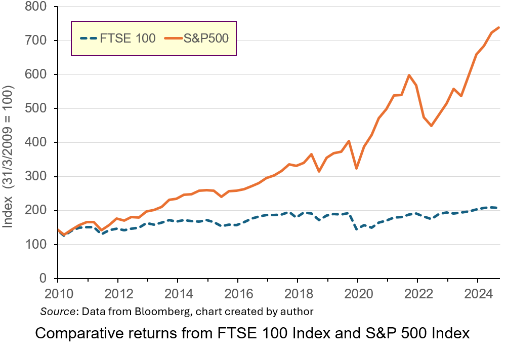
Investment in the S&P 500 Index over the period would have produced annualised rates of return of 14.35%, more than double that from the FTSE 100 Index. Part of this underperformance is due to the industrial mix of the listed companies: low-growth energy and mining compared to the high-growth technology sectors in the USA. This has led to the perception that London is not a place for firms to list, particularly those in high-growth sectors.
In 2024, 88 companies choose to delist or transfer their primary listing elsewhere. Only 18 took their place. Several big companies from a range of industries, including Ashtead, Flutter and CRH have transferred their primary listing to New York or have plans to do so.
 The new Labour government views stimulating higher levels of investment though the London market as an important element in its drive to boost productivity and growth in the UK. Recently, it has been reported that investment institutions have been lobbying the UK government to reduce significantly the tax-free allowance for Cash Individual Savings Accounts (ISAs) as a way to encourage more of UK households’ savings to be channelled through the UK stock market.
Currently, UK savers can save up to £20 000 annually into ISAs without paying tax on the interest earned. This can be held solely in Cash ISAs, or in a combination of Cash plus Stocks and Shares ISAs. The tax-free instruments which were introduced by a Labour government in 1999 to encourage higher savings have proved immensely popular. Data from Paragon Bank indicate that over £350 billion are held in these accounts. However, under the new proposals, the amount which would be allowed to be saved as cash has been rumoured to be cut to £4000 per year, with the hope that some of it will be invested in the UK stock market.
The proposals have proved controversial, with high-profile figures voicing opposition. In this blog, we’ll analyse the reasons behind the proposal and discuss whether it will have the desired effect of stimulating higher levels of investment. We’ll also discuss other proposed policies for making the LSE a more effective channel for investment flows to boost economic growth.
Stock markets and the saving and investment channel
 The main reason for the proposed ISA change is to encourage more investment in the UK stock market. By reducing the amount which can be saved in Cash ISAs, the government hopes to encourage savers to invest in Stocks and Shares ISAs instead, particularly ones linked to the UK market. This would increase the amount of finance capital in the market, thereby boosting its liquidity. This would then make it an attractive place for young, vibrant UK and foreign companies to list.
An active, liquid secondary market in shares is important to attract firms to list on stock exchanges by issuing shares to outside investors. Traditionally, this channel has been important to the growth and development of firms.
Existing savings in Cash ISAs are deposited with financial institutions such as banks and building societies. Through the credit-creation process such funds can be used to finance productive investment. In countries like the UK, lending by financial institutions is an important way that investment is financed, particularly for small and medium-sized enterprises. However, scale limits, regulatory restrictions and the need to diversify lending properly means that there are limits to the financing available for company investment through these institutions.
Capital markets like the LSE are intended to meet these larger-scale requirements. Financial claims, such as debt and equity, are divided into atomised instruments and sold to outside investors to fund investment and business growth.
 Further, the desire for a capital injection to finance growth is not the only reason that firms seek stock market listings. Founders of companies may have a lot of wealth invested in the equity of their firms. Selling some of their equity to outside investors through a stock market listing is a way of diversifying their wealth. However, if they are to maximise the potential sale price, there must be an active, liquid secondary market to encourage investors to buy shares in the primary market.
Proponents of reform want to encourage a greater appetite for risk among UK investors, which will produce more savings being channelled through the LSE.
One issue is whether savers will respond in the way anticipated and channel more funds through the UK stock market. Many savers like the security of Cash ISAs. Such vehicles offer a low-risk/low-return combination, which savers like because the tax benefits boost returns. A survey by the Nottingham Building Society found that a substantial number of Cash ISA savers are concerned that the proposed changes could affect their ability to save for important financial goals, such as buying a house or building an emergency fund. Higher-risk Stocks and Shares ISAs are not suitable for such savings because of the potential to lose the initial amount invested. Many may not be prepared to do so and one-third suggested they would save less overall.
According to the survey, only 38% of Cash ISA holders said they would consider investing in Stocks and Shares ISAs if the Cash ISA allowance were reduced. It may be difficult to alter such risk-averse preferences given the average amount saved through ISAs and demographics. In 2022/23, the average amount subscribed to ISAs was £5000. This does not suggest that average households have a significant surplus of cash that they may want to investment at a high risk through the stock market. Indeed, many may want to have access to the cash at short notice and so are not prepared to forgo liquidity for the time needed to accrue the benefits of compounding which stock market investing produces.
 Demographics may also play a role in this. Many of those who save more are now retired, or near retirement. They are less likely to see the appeal of compounding returns over long periods through investment in shares. Instead, with shorter investment horizons, they may only see the potential for losses associated with Stocks and Shares ISAs. Indeed, they will be starting to liquidate their long-term positions to draw income in retirement. Therefore, they may save less.
For others, who may be prepared to accept the additional risk, with the prospect of higher returns in the way that advocates of the reform hope for, the reduction in the Cash ISA allowance does not necessarily mean that they will invest in Stocks and Shares ISAs linked to the UK market. Since returns from the UK market have lagged international competitors, it may be that savers will channel their savings to those international markets, particularly in the USA, where the risk–return relationship has been more rewarding. Doing so has been made much easier and cheaper through a combination of economic forces including technological advances, regulatory changes and increased competition. This makes it much easier for UK savers to channel investment funds to wherever potential return is highest. At the moment, this is unlikely to be the UK, meaning that the anticipated boost to investment funds may not be as much as anticipated.
Critics of the proposal also question the motives of investment fund managers who have been lobbying government. They argue that the reforms will mean that many people who do now choose to save in Stocks and Shares ISAs will buy funds managed by fund managers who will receive fees for doing so. Critics argue that it is the prospect of higher fees which is the real motive behind the lobbying, not any desire to boost investment and growth.
What alternatives are available to boost the London Stock Exchange
 The low valuations of LSE-listed companies compared to their international counterparts, particularly those in the USA, has discouraged growing firms from listing in London. To address this, there have been calls to enhance corporate governance standards and reduce regulatory burdens for listed companies.
This has already been recognised by the authorities. In 2024, UK regulators approved the biggest overhaul of rules regulating London-listed companies. The new listing rules will hand more power to company bosses to make decisions without shareholder votes. They will give companies more flexibility to adopt dual-class share structures used by founders and venture capital firms to give themselves stronger voting rights than other investors. This is particularly popular for founders who want to diversify their wealth without sacrificing control and is used frequently by tech companies and venture capitalists when listing in the USA. Such reforms may attract more companies in high-growth sectors to list in London.
Tax policies which provide the right incentives to buy and sell shares could also encourage more investment in the LSE. For instance, the repeal in the mid-1990s of the preferential tax treatment of dividend income for UK pension funds and insurance companies is seen as a major factor in discouraging those institutions from investing more funds in the London market. Since tax on capital gains is only liable when they are realised, this reduces their present value versus the equivalent amount on dividends.
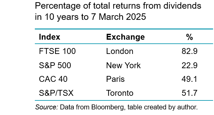
As the following table illustrates, given the significantly higher percentage of total returns derived from dividends in the LSE compared to other exchanges, the equal tax treatment of dividend and capital gains provides an incentive to seek jurisdictions where capital gains predominate. This is what UK pension funds have done. Data from the Office of National Statistics show that in 2024, 77% of UK occupational pensions equity investments were overseas.
Reinstating this tax benefit could stimulate greater demand for UK equity from this significant sector, boosting liquidity in the London market. Allied to this are proposals from the UK government to consolidate the fragmented UK pension industry to achieve greater scale economies in that channel for investment. This can reduce financing costs, boosting the marginal return from UK investments for these funds, encouraging greater investment in the UK market (ceteris paribus).
Further, the 2.5% stamp duty on share purchases has been viewed as another disincentive for both retail and institutional investors to engage in security trading on the London Stock Exchange. The duty, which is much higher than in peer economies, effectively raises the expected rate of return on UK equites which depresses perceptions of their values and prices. Its removal may raise trading volumes, improving the liquidity of the market and be offset by increased tax revenues in the future. However, the Treasury suggests that the removal of stamp duty is doubtful, since it would create a significant hole in the UK government’s budget.
 Ultimately, many of these reforms may have limited impact on investment. Efforts to boost confidence in the stock market will depend on improving the overall economic environment in the UK. Therefore, it will be the wider policies promoting growth in general which will increase the rates of return offered by London-listed firms and be more significant to attracting capital to London.
However, many of these are controversial themselves, such as relaxing laws around planning permissions and addressing business uncertainties around post-Brexit trading arrangements with the European Union. These broader economic measures could help make the UK generally, and the LSE specifically, more appealing to both domestic and international investors.
Conclusion
The UK government’s proposal to reduce the Cash ISA allowance is part of a broader strategy to boost investment in the stock market and stimulate economic growth. While this change could lead to more capital being directed towards productive investments, it also poses challenges for savers who like the security and simplicity of Cash ISAs.
The ultimate impact will depend on how savers respond to these changes. The potential reduction in overall savings rates could counteract some of the intended benefits. Further, the extent to which they are prepared to channel their savings into UK-listed companies will be important. If many seek higher returns elsewhere, the impact on the UK stock market may be limited. In any case, policies to address the problems of the UK stock market will only work if the wider issues associated with UK productivity and growth are addressed.
Articles
Data
Questions
- Explain how banks use cash ISAs to finance investment through credit creation.
- What do stock markets offer which may boost investment and economic growth?
- What are the issues with the London Stock Exchange which is making it unattractive for raising finance?
- How is the rumoured ISA reform intended to help address these issues?
- Analyse the extent to which it will do so.
- How might some of the broader reforms proposed by the UK government influence rate of return on UK equities and attract capital?
 In an interview with Joe Rogan for his podcast, The Joe Rogan Experience, just before the US election, Donald Trump stated that, “To me, the most beautiful word – and I’ve said this for the last couple of weeks – in the dictionary today and any is the word ‘tariff’. It’s more beautiful than love; it’s more beautiful than anything. It’s the most beautiful word. This country can become rich with the use, the proper use of tariffs.”
President-elect Trump has stated that he will impose tariffs on imports of 10% or 20%, with 60% and 100% tariffs on imports from China and Mexico, respectively. This protection for US industries, combined with lighter regulation, will, he claims, provide a stimulus to the economy and help create jobs. The revenues will also help to reduce America’s budget deficit.
But it is not that straightforward.
Problems with tariffs for the USA
 Imposing tariffs is likely to reduce international trade. But international trade brings net benefits, which are distributed between the participants according to the terms of trade. This is the law of comparative advantage.
In the simple two-country case, the law states that, provided the opportunity costs of producing various goods differ between the two countries, both of them can gain from mutual trade if they specialise in producing (and exporting) those goods that have relatively low opportunity costs compared with the other country. The total production and consumption of the two countries will be higher.
So if the USA has a comparative advantage in various manufactured products and a trading partner has a comparative advantage in tropical food products, such as coffee or bananas, both can gain by specialisation and trade.
If tariffs are imposed and trade is thereby reduced between the USA and its trading partners, there will be a net loss, as production will switch from lower-cost production to higher-cost production. The higher costs of less efficient production in the USA will lead to higher prices for those goods than if they were imported.
 At the same time, goods that are still imported will be more expensive as the price will include the tariff. Some of this may be borne by the importer, meaning that only part of the tariff is passed on to the consumer. The incidence of the tariff between consumer and importer will depend on price elasticities of demand and supply. Nevertheless, imports will still be more expensive, allowing the domestically-produced substitutes to rise in price too, albeit probably by not so much. According to work by Kimberly Clausing and Mary E Lovely for the Peterson Institute (see link in Articles below), Trump’s proposals to raise tariffs would cost the typical American household over $2600 a year.
The net effect will be a rise in inflation – at least temporarily. Yet one of Donald Trump’s pledges is to reduce inflation. Higher inflation will, in turn, encourage the Fed to raise interest rates, which will dampen investment and economic growth.
Donald Trump tends to behave transactionally rather than ideologically. He is probably hoping that a rapid introduction of tariffs will then give the USA a strong bargaining position with foreign countries to trade more fairly. He is also hoping that protecting US industries by the use of tariffs, especially when coupled with deregulation, will encourage greater investment and thereby faster growth.
Much will depend on how other countries respond. If they respond by raising tariffs on US exports, any gain to industries from protection from imports will be offset by a loss to exporters.
A trade war, with higher tariffs, will lead to a net loss in global GDP. It is a negative sum game. In such a ‘game’, it is possible for one ‘player’ (country) to gain, but the loss to the other players (countries) will be greater than that gain.
 Donald Trump is hoping that by ‘winning’ such a game, the USA could still come out better off. But the gain from higher investment, output and employment in the protected industries would have to outweigh the losses to exporting industries and from higher import prices.
The first Trump administration (2017–21), as part of its ‘America First’ programme, imposed large-scale tariffs on Chinese imports and on steel and aluminium from across the world. There was wide-scale retaliation by other countries with tariffs imposed on a range of US exports. There was a net loss to world income, including US GDP.
Problems with US tariffs for the rest of the world
The imposition of tariffs by the USA will have considerable effects on other countries. The higher the tariffs and the more that countries rely on exports to the USA, the bigger will the effect be. China and Mexico are likely to be the biggest losers as they face the highest tariffs and the USA is a major customer. In 2023, US imports from China were worth $427bn, while US exports to China were worth just $148bn – only 34.6% of the value of imports. The percentage is estimated to be even lower for 2024 at around 32%. In 2023, China’s exports to the USA accounted for 12.6% of its total exports; Mexico’s exports to the USA accounted for 82.7% of its total exports.
It is possible that higher tariffs could be extended beyond China to other Asian countries, such as Vietnam, South Korea, Taiwan, India and Indonesia. These countries typically run trade surpluses with the USA. Also, many of the products from these countries include Chinese components.
As far as the UK is concerned, the proposed tariffs would cause significant falls in trade. According to research by Nicolò Tamberi at the University of Sussex (see link below in Articles):
The UK’s exports to the world could fall by £22 billion (–2.6%) and imports by £1.4 (–0.16%), with significant variations across sectors. Some sectors, like fishing and petroleum, are particularly hard-hit due to their high sensitivity to tariff changes, while others, such as textiles, benefit from trade diversion as the US shifts demand away from China.
Other badly affected sectors would include mining, pharmaceuticals, finance and insurance, and business services. The overall effect, according to the research, would be to reduce UK output by just under 1%.
Countries are likely to respond to US tariffs by imposing their own tariffs on US imports. World Trade Organization rules permit the use of retaliatory tariffs equivalent to those imposed by the USA. The more aggressive the resulting trade war, the bigger would be the fall in world trade and GDP.
The EU is planning to negotiate with Trump to avoid a trade war, but officials are preparing the details of retaliatory measures should the future Trump administration impose the threatened tariffs. The EU response is likely to be strong.
Articles
 The Most Beautiful Word In The Dictionary: Tariffs
YouTube, Joe Rogan and Donald Trump
- The exact thing that helped Trump win could become a big problem for his presidency
CNN, Matt Egan (7/11/24)
- Trump’s New Trade War With China Is Coming
Newsweek, Micah McCartney (9/11/24)
- Trump tariff threat looms large on several Asian countries – not just China – says Goldman Sachs
CNBC, Lee Ying Shan (11/11/24)
- Trump’s bigger tariff proposals would cost the typical American household over $2,600 a year
Peterson Institute for International Economics, Kimberly Clausing and Mary E Lovely (21/8/24)
- More tariffs, less red tape: what Trump will mean for key global industries
The Guardian, Jasper Jolly, Dan Milmo, Jillian Ambrose and Jack Simpson (7/11/24)
- Trump tariffs would halve UK growth and push up prices, says thinktank
The Guardian, Larry Elliott (6/11/24)
- China is trying to fix its economy – Trump could derail those plans
BBC News, João da Silva (8/11/24)
- Trump tariffs could cost UK £22bn of exports
BBC News, Faisal Islam & Tom Espiner (8/11/24)
- Trump to target EU over UK in trade war as he wants to see ‘successful Brexit’, former staffer claims
Independent, Millie Cooke (11/11/24)
- EU’s trade war nightmare gets real as Trump triumphs
Politico, Camille Gijs (6/11/24)
- Will Trump impose his tariffs? They could reduce the UK’s exports by £22 billion.
Centre for Inclusive Trade Policy, University of Sussex, Nicolò Tamberi (8/11/24)
- Three possible futures for the global economy if Trump brings in new trade tariffs
The Conversation, Agelos Delis and Sami Bensassi (17/12/24)
Questions
- Explain why, according to the law of comparative advantage, all countries can gain from trade.
- In what ways may the imposition of tariffs benefit particular sections of an economy?
- Is it in countries’ interests to retaliate if the USA imposes tariffs on their exports to the USA?
- Why is a trade war a ‘negative sum game’?
- Should the UK align with the EU in resisting President-elect Trump’s trade policy or should it seek independently to make a free-trade deal with the USA? is it possible to do both?
- What should China do in response to US threats to impose tariffs of 60% or more on Chinese imports to the USA?
 On 25 October 2024, Moody’s, one of the major credit ratings agencies, announced that it was downgrading France’s economic outlook to negative. This was its first downgrading of France since 2012. It followed a similar revision by Fitch’s, another ratings agency, on 11 October.
While Fitch’s announcement did not have a significant impact on the yields of French government bonds, expectations around Moody’s did. In the week preceding the announcement, the net increases in the yield on generic 10-year government debt was approximately 9 basis points (0.09 percentage points). On the day itself, the yield rose by approximately 5.6 basis points (0.056 percentage points).
The yield rose further throughout the rest of October, finishing nearly 0.25 percentage points above its level at the start of the month. However, as Figure 1 illustrates, these increases are part of a longer-term trend of rising yields for French government debt (click here for a PowerPoint).
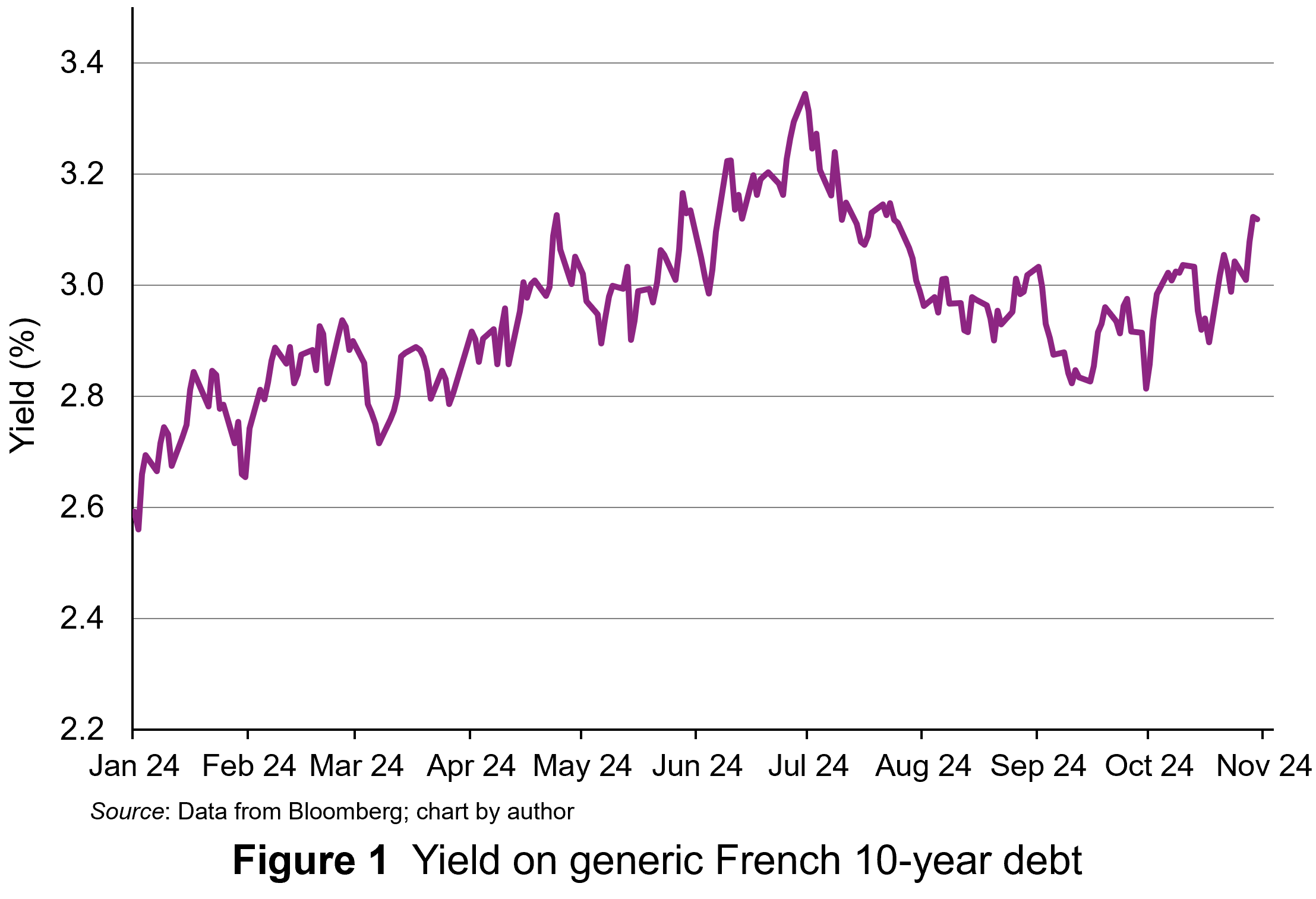 The yield on 10-year French government debt began 2024 at 2.56% and had an upward trend for the first half of the year. The yield peaked at 3.34% on 1 July. It then fell back below 3% for a while. The negative economic outlook then pushed yields back above 3% and they finished October at 3.12%, half a percentage point above the level at the start of the year. This represents a significant increase in borrowing costs for the French government.
In this blog, we will explain why the changes in France’s economic outlook translate into increases in yields for French government bonds. We will also analyse why yields have increased and examine the prospects for the markets in French government bonds.
Pricing signals of bond yields
A bond is a tradable debt instrument issued by governments to finance budget deficits – the difference between tax receipts and spending. Like any financial instruments, investment in bonds involves a commitment of funds today in anticipation of interest payments through time as compensation, with a repayment of its redemption value on the date the bond matures.
Since the cash flows associated with holding a bond occur at different points in time, discounted cash flow analysis is used to determine its value. This gives the present value of the cash flows discounted at the appropriate expected rate of return. In equilibrium this will be equal to the bond’s market price, as the following equation shows.

Where:
P = the equilibrium price of the bond
C = cash coupon payments
M = redemption value at maturity
r = yield (expected rate of return in equilibrium.
Interest payments tend to be fixed at the time a bond is issued and reflect investors’ expected rate of return, expressed as the yield in bond markets. This is determined by prevailing interest rates and perceived risk. Over time, changes in interest rates and perceptions of risk will change the expected rate of return (yield), which will, in turn, change the present value of the cash flows, and hence fundamental value.
Prices move in response to changes in fundamental value and since this happens frequently, this means that prices change a lot. For bonds, as the coupon payments (C each year and the redemption price () are fixed, the only factor that can change is the expected rate of return (yield). This is reflected in the observed yield at each price.
 If the expected rate of return rises, this increases the discount rate applied to future cash flows and reduces their present value. At the current price, the fixed coupon is not sufficient to compensate investors. So, investors sell the bonds and price falls until it reaches a point where the yield offered is equal to that required. The reverse happens if the expected rate of return falls.
The significant risk associated with bonds is credit default risk – the risk that the debt will not be repaid. The potential for credit default is a significant influence of the compensation investors require for holding debt instruments like bonds (ceteris paribus). An increase in expected credit default risk will increase the expected return (compensation). This will be reflected in a lower price and higher yield.
Normally, with the bonds issued by high-income countries, such as those in Europe and North America, the risk of default is extremely low. However, if a country’s annual deficits or accumulated debt increase to what markets consider to be unsustainable levels, the perceived risk of default may rise. Countries’ levels of risk are rated by international ratings agencies, such as Moody’s and Fitch. Investors pay a lot of attention to the information provided by such agencies.
Moody’s downgrade in its economic outlook for France from ‘stable’ to ‘negative’ indicated weak economic performance and higher credit default risk. This revision rippled through bond markets as investors adjusted their views of the country’s economic risk. The rise in yields observed is a signal that bond investors perceive higher credit default risk associated with French government debt and are demanding a higher rates of return as compensation.
Why has France’s credit default risk premium risen now?
As we have seen, credit default risk is not normally considered a significant issue for sovereign borrowers like France. Some of the issue around perceived credit default risk for the French government relate to the size of the French government’s deficit and the projections for it. Following a spike in borrowing associated with the COVID-19 pandemic in 2020, the annual government budget deficit and the overall level of debt as percentages of GDP have remained high. The annual deficit is projected to be 6% for 2024 and still 5% for 2025. The ratio of outstanding French government debt to Gross Domestic Product (GDP) ballooned to 123% in 2020 and is still expected to be 115% by the end of 2025. France has been put on notice to reduce its debt towards the Eurozone limit of 60% of GDP.
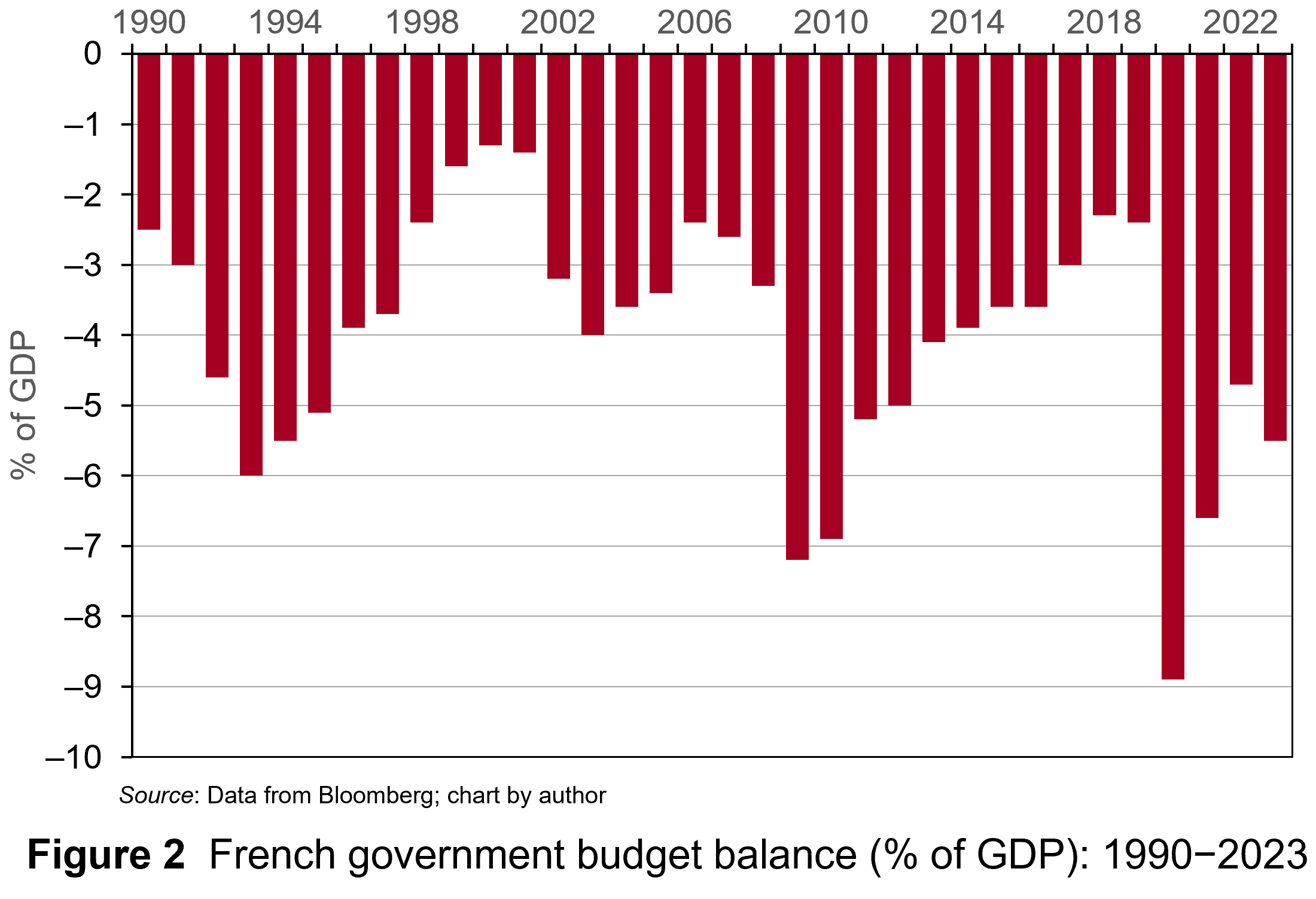 Governments in France last achieved a balanced budget in 1974. They have run deficits ever since. Figure 2 illustrates the French government budget deficits from 1990 to 2023 (click here for a PowerPoint). The figure shows that France experienced deficits in the past similar to today’s. These, however, did not tend to worry bond markets too much.
So why are investors currently worried? This stems from France’s debt mountain and from concerns that the government will not be able to deal with it. Investors are concerned that both weak growth and increasingly volatile politics will thwart efforts to reduce debt levels.
Let’s take growth. Even by contemporary European standards, France’s growth prospects are anaemic. GDP is expected to grow by just 1.1% for 2024 and 1% for 2025. Both consumer and business confidence are low. None of this suggests a growth spurt soon which will boost the tax revenues of the French government sufficiently to address the deficit.
 Further, political instability has grown due to the inconclusive parliamentary elections which Emmanuel Macron surprisingly called in July. No single political grouping has a majority and the President has appointed a Centrist Prime Minister, Michel Barnier (the former EU Brexit negotiator). His government is trying to pass a budget through the Assemblée Nationale involving a mixture of spending cuts and tax hikes which amount to savings of €60 billion ($66 billion). This is equivalent to 2% of GDP.
The parliamentary path of the budget bill is set to be torturous with both the left and right wing blocs in the Assemblée opposing most of the provisions. Debate in the Assemblée Nationale and Senate are expected to drag on into December, with the real prospect that the government may have to use presidential decree to pass the budget. Commentators argue that this will fuel further political chaos.
France looks more like Southern Europe
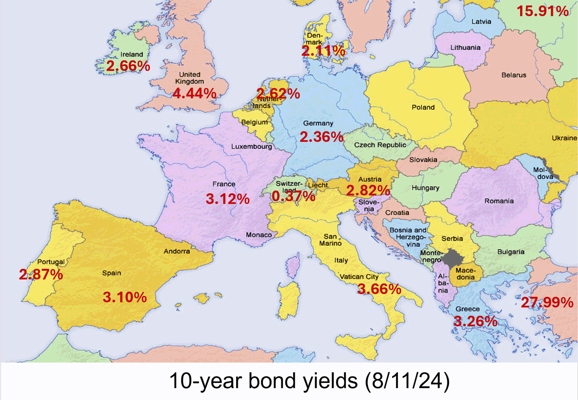 In the past, bond investors were more tolerant of France’s budget deficits. French government bonds were attractive options for investors wanting to hold euro-denominated bonds while avoiding riskier Southern European countries such as Greece, Italy, Portugal and Spain. Since France has run persistent government deficits for a long time, it offered bond investors a more liquid market than more fiscally-parsimonious Northern European neighbours, such as Germany and the Netherlands. Consequently, France’s debt instruments offered a slight risk premium on the yields for those countries.
However, that has changed. France’s credit default risk premium is rising to levels comparable to its Southern neighbours. On 26 September 2024, the yield on generic French government 10-year debt rose above its Spanish equivalent for the first time since 2008.
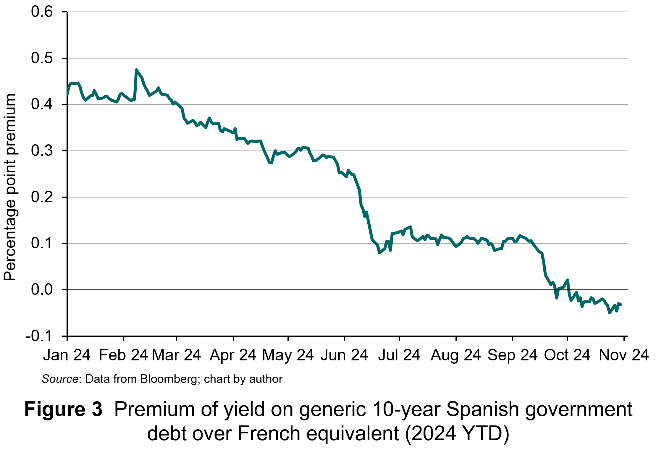 As Figure 3 illustrates, this was the culmination of a trend evident throughout 2024, with the difference in yields between the two declining steadily (click here for a PowerPoint). At the start of the year, the yield on Spanish debt offered a 40 basis points premium over the French equivalent. By October, the yield on Spanish debt was consistently below that of French debt. All of this is due to bond investors’ rising expectations about France’s credit default risk. Now, France’s borrowing costs are not only above Spain, but also closer to those of Greece and Italy than of Germany.
Strikingly, Spain’s budget deficit was 3.5% in 2023 and is expected to narrow to 2.6% by 2025. The percentage of total debt to GDP is 104% and falling. Moreover, following Spain’s inconclusive election in 2023, the caretaker government put forward budgetary plans involving fiscal tightening without the need for legislation. This avoided the political wrangling France is facing.
For France, these developments raise the prospect of yields rising further as bond investors now see alternatives to French government debt in the form of Spain’s. This country have already undertaken the painful fiscal adjustments that France seems incapable of completing.
Articles
Data
Questions
- What is credit default risk?
- Explain why higher credit default risk is associated with higher yields on France’s government debt.
- Why would low economic growth worsen the government’s budget deficit?
- Why would political instability increase credit default risk?
- What has happened to investors’ perceptions of the risk associated with French government debt relative to Spain’s?
- How has this manifested itself in the relative yields of the two countries’ government debt?
 We continue to live through incredibly turbulent times. In the past decade or so we have experienced a global financial crisis, a global health emergency, seen the UK’s departure from the European Union, and witnessed increasing levels of geopolitical tension and conflict. Add to this the effects from the climate emergency and it easy to see why the issue of economic uncertainty is so important when thinking about a country’s economic prospects.
In this blog we consider how we can capture this uncertainty through a World Uncertainty Index and the ways by which economic uncertainty impacts on the macroeconomic environment.
World Uncertainty Index
Hites Ahir, Nicholas Bloom and Davide Furceri have constructed a measure of uncertainty known as the World Uncertainty Index (WUI). This tracks uncertainty around the world using the process of ‘text mining’ the country reports produced by the Economist Intelligence Unit. The words searched for are ‘uncertain’, ‘uncertainty’ and ‘uncertainties’ and a tally is recorded based on the number of times they occur per 1000 words of text. To produce the index this figure is then multiplied up by 100 000. A higher number therefore indicates a greater level of uncertainty. For more information on the construction of the index see the 2022 article by Ahir, Bloom and Furceri linked below.
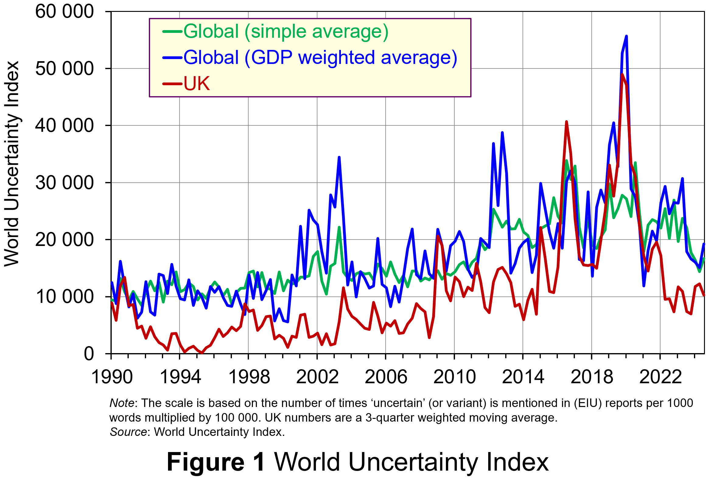 Figure 1 (click here for a PowerPoint) shows the WUI both globally and in the UK quarterly since 1991. The global index covers 143 countries and is presented as both a simple average and a GDP weighted average. The UK WUI is also shown. This is a three-quarter weighted average, the authors’ preferred measure for individual countries, where increasing weights of 0.1, 0.3 and 0.6 are used for the three most recent quarters.
From Figure 1 we can see how the level of uncertainty has been particularly volatile over the past decade or more. Events such as the sovereign debt crisis in parts of Europe in the early 2010s, the Brexit referendum in 2016, the COVID-pandemic in 2020–21 and the invasion of Ukraine in 2022 all played their part in affecting uncertainty domestically and internationally.
Uncertainty, risk-aversion and aggregate demand
Now the question turns to how uncertainty affects economies. One way of addressing this is to think about ways in which uncertainty affects the choices that people and businesses make. In doing so, we could think about the impact of uncertainty on components of aggregate demand, such as household consumption and investment, or capital expenditures by firms.
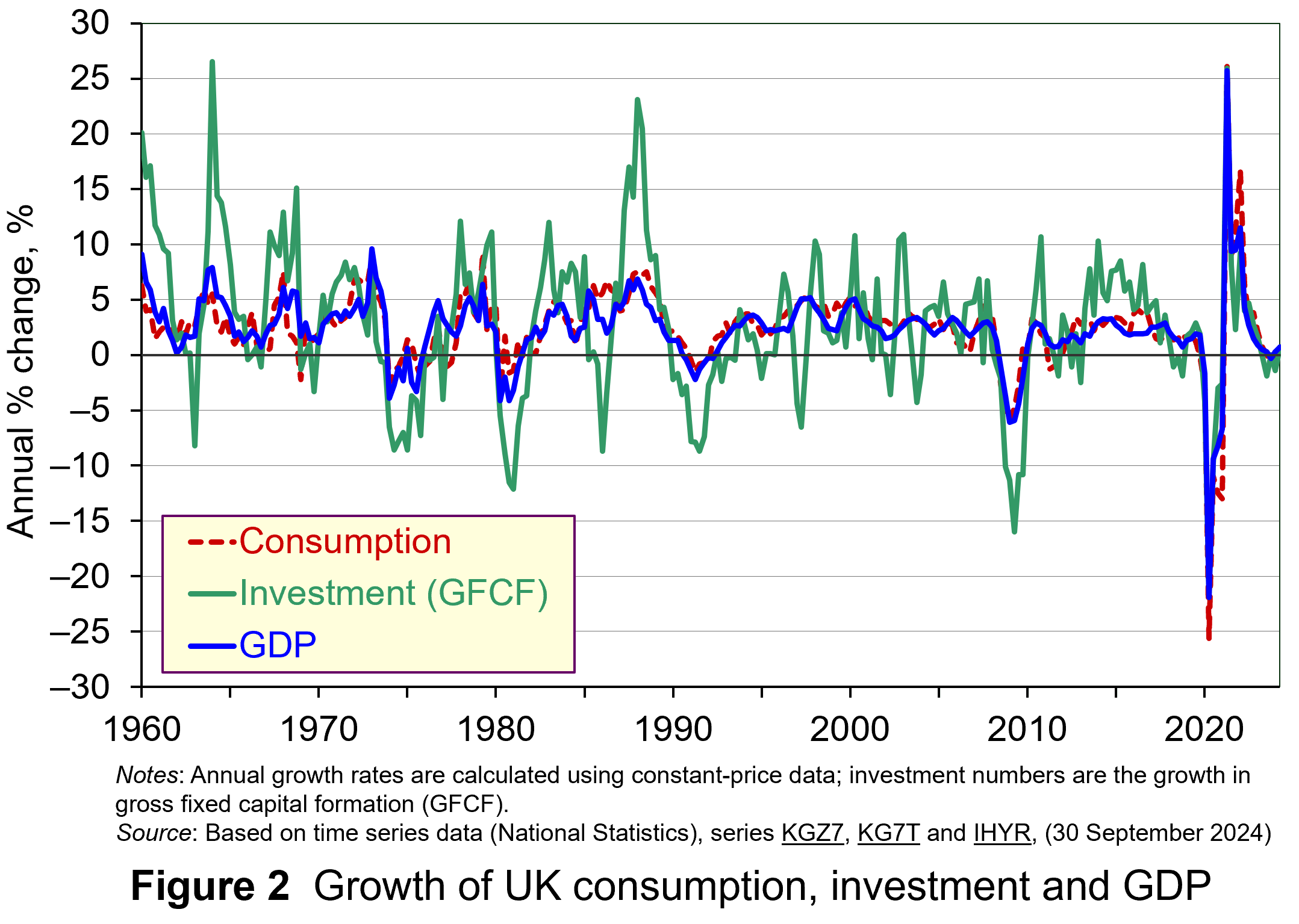 As Figure 2 shows (click here for a PowerPoint), investment is particularly volatile, and much more so than household spending. Some of this can be attributed to the ‘lumpiness’ of investment decisions since these expenditures tend to be characterised by indivisibility and irreversibility. This means that they are often relatively costly to finance and are ‘all or nothing’ decisions. In the context of uncertainty, it can make sense therefore for firms to wait for news that makes the future clearer. In this sense, we can think of uncertainty rather like a fog that firms are peering through. The thicker the fog, the more uncertain the future and the more cautious firms are likely to be.
The greater caution that many firms are likely to adopt in more uncertain times is consistent with the property of risk-aversion that we often attribute to a range of economic agents. When applied to household spending decisions, risk-aversion is often used to explain why households are willing to hold a buffer stock of savings to self-insure against unforeseen events and their future financial outcomes being worse than expected. Hence, in more uncertain times households are likely to want to increase this buffer further.
 The theory of buffer-stock saving was popularised by Christopher Carroll in 1992 (see link below). It implies that in the presence of uncertainty, people are prepared to consume less today in order to increase levels of saving, pay off existing debts, or borrow less relative to that in the absence of uncertainty. The extent of the buffer of financial wealth that people want to hold will depend on their own appetite for risk, the level of uncertainty, and the moderating effect from their own impatience and, hence, present bias for consuming today.
Risk aversion is consistent with the property of diminishing marginal utility of income or consumption. In other words, as people’s total spending volumes increase, their levels of utility or satisfaction increase but at an increasingly slower rate. It is this which explains why individuals are willing to engage with the financial system to reallocate their expected life-time earnings and have a smoother consumption profile than would otherwise be the case from their fluctuating incomes.
Yet diminishing marginal utility not only explains consumption smoothing, but also why people are willing to engage with the financial system to have financial buffers as self-insurance. It explains why people save more or borrow less today than suggested by our base-line consumption smoothing model. It is the result of people’s greater dislike (and loss of utility) from their financial affairs being worse than expected than their like (and additional utility) from them being better than expected. This tendency is only likely to increase the more uncertain times are. The result is that uncertainty tends to lower household consumption with perhaps ‘big-ticket items’, such as cars, furniture, and expensive electronic goods, being particularly sensitive to uncertainty.
Uncertainty and confidence
Uncertainty does not just affect risk; it also affects confidence. Risk and confidence are often considered together, not least because their effects in generating and transmitting shocks can be difficult to disentangle.
We can think of confidence as capturing our mood or sentiment, particularly with respect to future economic developments. Figure 3 plots the Uncertainty Index for the UK alongside the OECD’s composite consumer and business confidence indicators. Values above 100 for the confidence indicators indicate greater confidence about the future economic situation and near-term business environment, while values below 100 indicate pessimism towards the future economic and business environments.
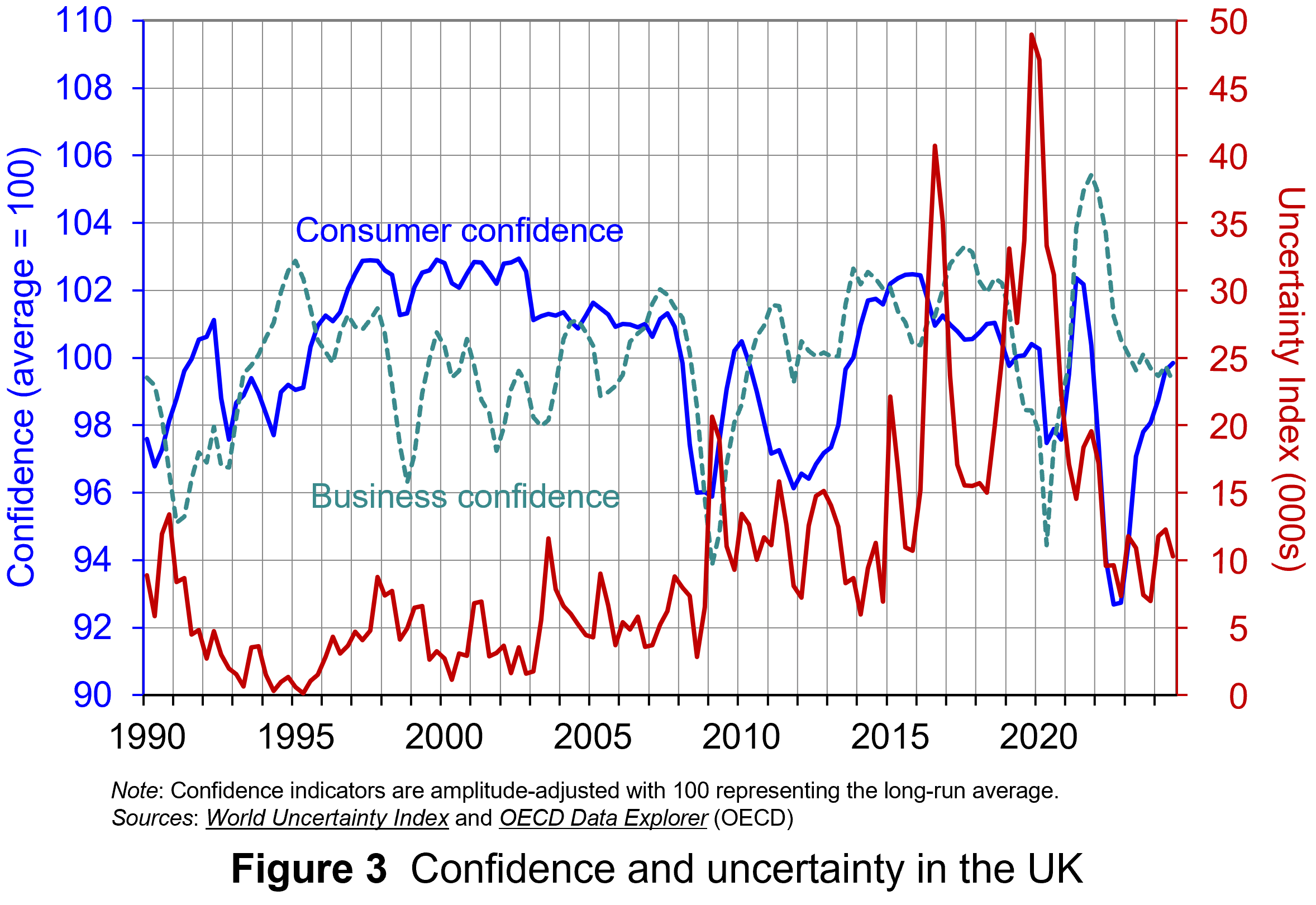 Figure 3 suggests that the relationship between confidence and uncertainty is rather more complex than perhaps is generally understood (click here for a PowerPoint). Haddow, Hare, Hooley and Shakir (see link below) argue that the evidence tends to point to changes in uncertainty affecting confidence, but with less evidence that changes in confidence affect uncertainty.
To illustrate this, consider the global financial crisis of the late 2000s. The argument can be made that the heightened uncertainty about future prospects for households and businesses helped to erode their confidence in the future. The result was that people and businesses revised down their expectations of the future (pessimism). However, although people were more pessimistic about the future, this was more likely to have been the result of uncertainty rather than the cause of further uncertainty.
Conclusion
For economists and policymakers alike, indicators of uncertainty, such as the Ahir, Bloom and Furceri World Uncertainty Index, are invaluable tools in understanding and forecasting behaviour and the likely economic outcomes that follow. Some uncertainty is inevitable, but the persistence of greater uncertainty since the global financial crisis of the late 2000s compares quite starkly with the relatively lower and more stable levels of uncertainty seen from the mid-1990s up to the crisis. Hence the recent frequency and size of changes in uncertainty show how important it to understand how uncertainty effects transmit through economies.
Academic papers
- The World Uncertainty Index
National Bureau of Economic Research, Working Paper 29763, Hites Ahir, Nicholas Bloom and Davide Furceri (February 2022)
- The Buffer-Stock Theory of Saving: Some Macroeconomic Evidence
Brookings Papers on Economic Activity, Christopher D Carroll (Vol 2, 1992)
- Macroeconomic uncertainty: what is it, how can we measure it and why does it matter?
Bank of England Quarterly Bulletin, 2013 Q2, Abigail Haddow, Chris Hare, John Hooley and Tamarah Shakir (13/6/13)
Articles
Data
Questions
- (a) Explain what is meant by the concept of diminishing marginal utility of consumption.
(b) Explain how this concept helps us to understand both consumption smoothing and the motivation to engage in buffer-stock saving.
- Explain the distinction between confidence and uncertainty when analysing macroeconomic shocks.
- Discuss which types of expenditures you think are likely to be most susceptible to uncertainty shocks.
- Discuss how economic uncertainty might affect productivity and the growth of potential output.
- How might the interconnectedness of economies affect the transmission of uncertainty effects through economies?
 The UK signed three trade deals in May – one with the USA, one with India and one with the EU. It is hoped by the government that these trade deals will provide a welcome boost to the UK economy.
 Perhaps the most significant new trade deal, however, is with the EU. This is a major advance on the current post-Brexit Trade and Cooperation Agreement (TCA). Under the TCA, there are no tariffs or quotas on UK goods exports to the EU or EU goods exports to the UK. However, to ensure that it is EU and UK business that benefits from these ‘trade preferences’, firms must show that their products fulfil ‘rules of origin’ requirements.
 Also, the TCA does not include free trade in services. The UK is a major exporter of services, including legal, financial, accounting, IT and engineering. It has a positive trade in services balance with the EU, unlike its negative trade in goods balance. Although some of the barriers which apply to other non-EU countries have been reduced for the UK in the TCA, UK service providers still face barriers which impose costs. For example, some EU countries limit the time that businesspeople providing services can stay in their countries to six months in any twelve. Also, since Brexit, UK artists and musicians have faced restrictions when touring and working in the EU. They can only work up to 90 out of every 180 days. This causes problems for longer tours and for musicians and crew who work in multiple bands or orchestras.
 The post-Brexit fishing deal between the UK and EU, which saw a reduction of 25% in EU fishing quotas in UK waters, will be extended for another 12 years. Many UK fishers, however, had hoped for scrapping EU access to UK waters. The deal also allows various sea foods, including certain shellfish, to be exported to the EU for the first time since Brexit.
 The new Labour government views stimulating higher levels of investment though the London market as an important element in its drive to boost productivity and growth in the UK. Recently, it has been reported that investment institutions have been lobbying the UK government to reduce significantly the tax-free allowance for Cash Individual Savings Accounts (ISAs) as a way to encourage more of UK households’ savings to be channelled through the UK stock market.
 The main reason for the proposed ISA change is to encourage more investment in the UK stock market. By reducing the amount which can be saved in Cash ISAs, the government hopes to encourage savers to invest in Stocks and Shares ISAs instead, particularly ones linked to the UK market. This would increase the amount of finance capital in the market, thereby boosting its liquidity. This would then make it an attractive place for young, vibrant UK and foreign companies to list.
  Further, the desire for a capital injection to finance growth is not the only reason that firms seek stock market listings. Founders of companies may have a lot of wealth invested in the equity of their firms. Selling some of their equity to outside investors through a stock market listing is a way of diversifying their wealth. However, if they are to maximise the potential sale price, there must be an active, liquid secondary market to encourage investors to buy shares in the primary market.
  Demographics may also play a role in this. Many of those who save more are now retired, or near retirement. They are less likely to see the appeal of compounding returns over long periods through investment in shares. Instead, with shorter investment horizons, they may only see the potential for losses associated with Stocks and Shares ISAs. Indeed, they will be starting to liquidate their long-term positions to draw income in retirement. Therefore, they may save less.
  The low valuations of LSE-listed companies compared to their international counterparts, particularly those in the USA, has discouraged growing firms from listing in London. To address this, there have been calls to enhance corporate governance standards and reduce regulatory burdens for listed companies.
 Ultimately, many of these reforms may have limited impact on investment. Efforts to boost confidence in the stock market will depend on improving the overall economic environment in the UK. Therefore, it will be the wider policies promoting growth in general which will increase the rates of return offered by London-listed firms and be more significant to attracting capital to London.
  In an interview with Joe Rogan for his podcast, The Joe Rogan Experience, just before the US election, Donald Trump stated that, “To me, the most beautiful word – and I’ve said this for the last couple of weeks – in the dictionary today and any is the word ‘tariff’. It’s more beautiful than love; it’s more beautiful than anything. It’s the most beautiful word. This country can become rich with the use, the proper use of tariffs.”
 Imposing tariffs is likely to reduce international trade. But international trade brings net benefits, which are distributed between the participants according to the terms of trade. This is the law of comparative advantage.
 Donald Trump is hoping that by ‘winning’ such a game, the USA could still come out better off. But the gain from higher investment, output and employment in the protected industries would have to outweigh the losses to exporting industries and from higher import prices.
 On 25 October 2024, Moody’s, one of the major credit ratings agencies, announced that it was downgrading France’s economic outlook to negative. This was its first downgrading of France since 2012. It followed a similar revision by Fitch’s, another ratings agency, on 11 October.
 The yield on 10-year French government debt began 2024 at 2.56% and had an upward trend for the first half of the year. The yield peaked at 3.34% on 1 July. It then fell back below 3% for a while. The negative economic outlook then pushed yields back above 3% and they finished October at 3.12%, half a percentage point above the level at the start of the year. This represents a significant increase in borrowing costs for the French government.
 If the expected rate of return rises, this increases the discount rate applied to future cash flows and reduces their present value. At the current price, the fixed coupon is not sufficient to compensate investors. So, investors sell the bonds and price falls until it reaches a point where the yield offered is equal to that required. The reverse happens if the expected rate of return falls.
  Governments in France last achieved a balanced budget in 1974. They have run deficits ever since. Figure 2 illustrates the French government budget deficits from 1990 to 2023 (click
  Further, political instability has grown due to the inconclusive parliamentary elections which Emmanuel Macron surprisingly called in July. No single political grouping has a majority and the President has appointed a Centrist Prime Minister, Michel Barnier (the former EU Brexit negotiator). His government is trying to pass a budget through the Assemblée Nationale involving a mixture of spending cuts and tax hikes which amount to savings of €60 billion ($66 billion). This is equivalent to 2% of GDP.
 In the past, bond investors were more tolerant of France’s budget deficits. French government bonds were attractive options for investors wanting to hold euro-denominated bonds while avoiding riskier Southern European countries such as Greece, Italy, Portugal and Spain. Since France has run persistent government deficits for a long time, it offered bond investors a more liquid market than more fiscally-parsimonious Northern European neighbours, such as Germany and the Netherlands. Consequently, France’s debt instruments offered a slight risk premium on the yields for those countries.
  As Figure 3 illustrates, this was the culmination of a trend evident throughout 2024, with the difference in yields between the two declining steadily (click
  We continue to live through incredibly turbulent times. In the past decade or so we have experienced a global financial crisis, a global health emergency, seen the UK’s departure from the European Union, and witnessed increasing levels of geopolitical tension and conflict. Add to this the effects from the climate emergency and it easy to see why the issue of economic uncertainty is so important when thinking about a country’s economic prospects.
 Figure 1 (click
  As Figure 2 shows (click
  The theory of buffer-stock saving was popularised by Christopher Carroll in 1992 (see link below). It implies that in the presence of uncertainty, people are prepared to consume less today in order to increase levels of saving, pay off existing debts, or borrow less relative to that in the absence of uncertainty. The extent of the buffer of financial wealth that people want to hold will depend on their own appetite for risk, the level of uncertainty, and the moderating effect from their own impatience and, hence, present bias for consuming today.
 Figure 3 suggests that the relationship between confidence and uncertainty is rather more complex than perhaps is generally understood (click