 In a blog from March 2023 (reproduced below), we saw how there has been growing pressure around the world for employers to move to a four-day week. Increasing numbers of companies have adopted the model of 80% of the hours for 100% of the pay.
As we see below, the model adopted has varied across companies, depending on what was seen as most suitable for them. Some give everyone Friday off; others let staff choose which day to have off; others let staff work 80% of the hours on a flexible basis. Firms adopting the model have generally found that productivity and revenue have increased, as has employee well-being. To date, over 200 employers in the UK, employing more than 5000 people, have adopted a permanent four-day week.
This concept of 100-80-100, namely 100% of pay for 80% of hours, but 100% of output, has been trialled in several countries. In Germany, after trials over 2024, 73% of the companies involved plan to continue with the new model, with the remaining 27% either making minor tweaks or yet to decide. Generally hourly productivity rose, and in many cases total output also rose. As the fourth article below states:
The primary causal factor for this intriguing revelation was simple – efficiency became the priority. Reports from the trial showed that the frequency and duration of meetings was reduced by 60%, which makes sense to anyone who works in an office – many meetings could have been a simple email. 25% of companies tested introduced new digitised ways of managing their workflow to optimise efficiency.
Original post
In two previous posts, one at the end of 2019 and one in July 2021, we looked at moves around the world to introduce a four-day working week, with no increase in hours on the days worked and no reduction in weekly pay. Firms would gain if increased worker energy and motivation resulted in a gain in output. They would also gain if fewer hours resulted in lower costs.
Workers would be likely to gain from less stress and burnout and a better work–life balance. What is more, firms’ and workers’ carbon footprint could be reduced as less time was spent at work and in commuting.
If the same output could be produced with fewer hours worked, this would represent an increase in labour productivity measured in output per hour.
The UK’s poor productivity record since 2008
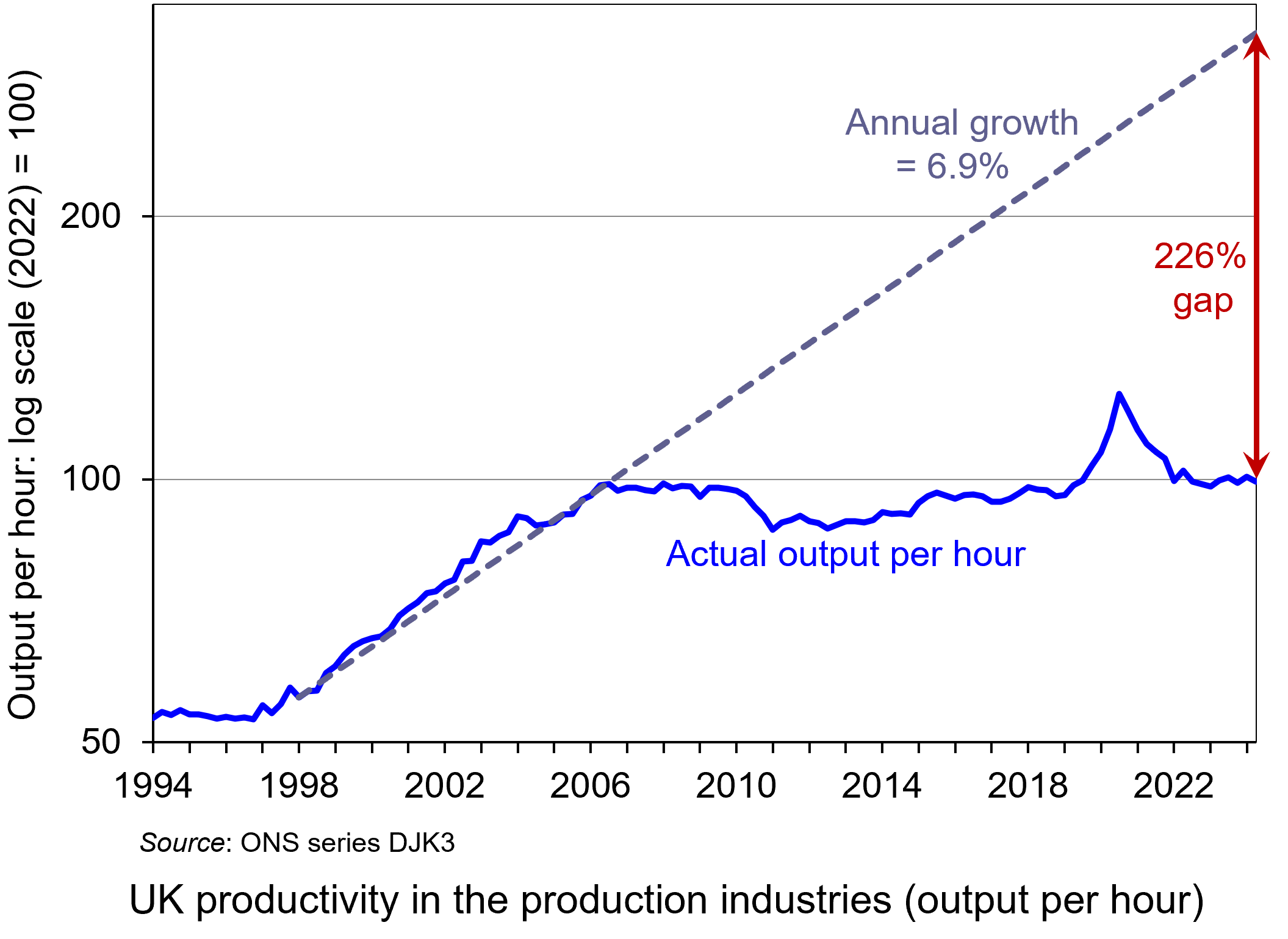 Since the financial crisis of 2007–8, the growth in UK productivity has been sluggish. This is illustrated in the chart, which looks at the production industries: i.e. it excludes services, where average productivity growth tends to be slower. The chart has been updated to 2024 Q2 – the latest data available. (Click here for a PowerPoint of the chart.)
Prior to the crisis, from 1998 to 2006, UK productivity in the production industries grew at an annual rate of 6.9%. From 2007 to the start of the pandemic in 2020, the average annual productivity growth rate in these industries was a mere 0.2%.
It grew rapidly for a short time at the start of the pandemic, but this was because many businesses temporarily shut down or went to part-time working, and many of these temporary job cuts were low-wage/low productivity jobs. If you take services, the effect was even stronger as sectors such as hospitality, leisure and retail were particularly affected and labour productivity in these sectors tends to be low. As industries opened up and took on more workers, so average productivity rapidly fell back. Since then productivity has flatlined.
If you project the average productivity growth rate from 1998 to 2007 of 6.9% forwards (see grey dashed line), then by 2024 Q3, output per hour in the production industries would have been 3.26 times higher than it actually was: a gap of 226%. This is a huge productivity gap.
 Productivity in the UK is lower than in many other competitor countries. According to the ONS, output per hour in the UK in 2021 was $59.14 in the UK. This compares with an average of $64.93 for the G7 countries, $66.75 in France, £68.30 in Germany, $74.84 in the USA, $84.46 in Norway and $128.21 in Ireland. It is lower, however, in Italy ($54.59), Canada ($53.97) and Japan ($47.28).
As we saw in the blog, The UK’s poor productivity record, low UK productivity is caused by a number of factors, not least the lack of investment in physical capital, both by private companies and in public infrastructure, and the lack of investment in training. Other factors include short-termist attitudes of both politicians and management and generally poor management practices. But one cause is the poor motivation of many workers and the feeling of being overworked. One solution to this is the four-day week.
Latest evidence on the four-day week
Results have just been released of a pilot programme involving 61 companies and non-profit organisations in the UK and nearly 3000 workers. They took part in a six-month trial of a four-day week, with no increase in hours on the days worked and no loss in pay for employees – in other words, 100% of the pay for 80% of the time. The trial was a success, with 91% of organisations planning to continue with the four-day week and a further 4% leaning towards doing so.
 The model adopted varied across companies, depending on what was seen as most suitable for them. Some gave everyone Friday off; others let staff choose which day to have off; others let staff work 80% of the hours on a flexible basis.
There was little difference in outcomes across different types of businesses. Compared with the same period last year, revenues rose by an average of 35%; sick days fell by two-thirds and 57% fewer staff left the firms. There were significant increases in well-being, with 39% saying they were less stressed, 40% that they were sleeping better; 75% that they had reduced levels of burnout and 54% that it was easier to achieve a good work–life balance. There were also positive environmental outcomes, with average commuting time falling by half an hour per week.
There is growing pressure around the world for employers to move to a four-day week and this pilot provides evidence that it significantly increases productivity and well-being.
Additional articles
Original set of articles
- Results from world’s largest 4 day week trial bring good news for the future of work
4 Day Week Global, Charlotte Lockhart (21/2/23)
- Four-day week: ‘major breakthrough’ as most UK firms in trial extend changes
The Guardian, Heather Stewart (21/2/23)
- Senedd committee backs four-day working week trial in Wales
The Guardian, Steven Morris (24/1/23)
- ‘Major breakthrough’: Most firms say they’ll stick with a four-day working week after successful trial
Sky News, Alice Porter (21/2/23)
- Major four-day week trial shows most companies see massive staff mental health benefits and profit increase
Independent, Anna Wise (21/2/23)
- Four-day week: Which countries have embraced it and how’s it going so far?
euronews, Josephine Joly and Luke Hurst (23/2/23)
- Firms stick to four-day week after trial ends
BBC News, Simon Read, Lucy Hooker & Emma Simpson (21/2/23)
- The climate benefits of a four-day workweek
BBC Future Planet, Giada Ferraglioni and Sergio Colombo (21/2/23)
- Four-day working week: why UK businesses and workers will continue with new work pattern, plus pros and cons
National World, Rochelle Barrand (22/2/23)
- Most companies in UK four-day week trial to continue with flexible working
Financial Times, Daniel Thomas and Emma Jacobs (21/2/23)
- The pros and cons of a four-day working week
Financial Times, Editorial (13/2/23)
- Explaining the UK’s productivity slowdown: Views of leading economists
VoxEU, Ethan Ilzetzki (11/3/20)
- Why the promised fourth industrial revolution hasn’t happened yet
The Conversation, Richard Markoff and Ralf Seifert (27/2/23)
Questions
- What are the possible advantages of moving to a four-day week?
- What are the possible disadvantages of moving to a four-day week?
- What types of companies or organisations are (a) most likely, (b) least likely to gain from a four-day week?
- Why has the UK’s productivity growth been lower than that of many of its major competitors?
- Why, if you use a log scale on the vertical axis, is a constant rate of growth shown as a straight line? What would a constant rate of growth line look like if you used a normal arithmetical scale for the vertical axis?
- Find out what is meant by the ‘fourth industrial revolution’. Does this hold out the hope of significant productivity improvements in the near future? (See, for example, last link above.)
 At an event at the London Palladium on 6 December staged to protest against elements in the recent Budget, the Conservative leader, Kemi Badenoch, was asked whether she would introduce a flat-rate income tax if the Conservatives were returned to government. She replied that it was a very attractive idea. But first the economy would need ‘rewiring’ so that the tax burden could be lightened.
A flat-rate income tax system could take various forms, but the main feature is that there is a single rate of income tax. The specific rate would depend on how much the government wanted to raise. Also it could apply to just income tax, or to both income tax and social insurance (national insurance contributions (NICs) in the UK), or to income tax, social insurance and the withdrawal rate of social benefits. It could also apply to local/state taxes as well as national/federal taxes.
Take the simplest case of a flat-rate income tax with no personal allowance. In this system the marginal and average rate of tax is the same for everyone. This is known as a proportional tax.
Most countries have a progressive income tax system. This normally involves personal allowances (i.e. a zero rate up to a certain level of income) and then various tax bands, with the marginal rate rising when particular tax thresholds are reached. In England, Wales and Northern Ireland, there are three tax bands: 20%, 40% and 45%. Thus the higher a person’s income is, the higher their average rate of tax.
A regressive tax, by contrast, would be one where the average rate of tax fell as incomes rose. The extreme case of a regressive tax would be a lump-sum tax (such as a TV or other licence), which would be same absolute amount for everyone liable to it, irrespective of their income. This was the case with the ‘poll tax’ (or Community Charge, to give it its official title), introduced by Margaret Thatcher’s government in 1989 in Scotland and 1990 in the rest of the UK. It was a local tax, with each taxpayer taxed the same fixed sum, with the precise amount being set by each local authority. After protests and riots, it was replaced in 1993 by the current system of local taxation (Council Tax) based on property values in bands.
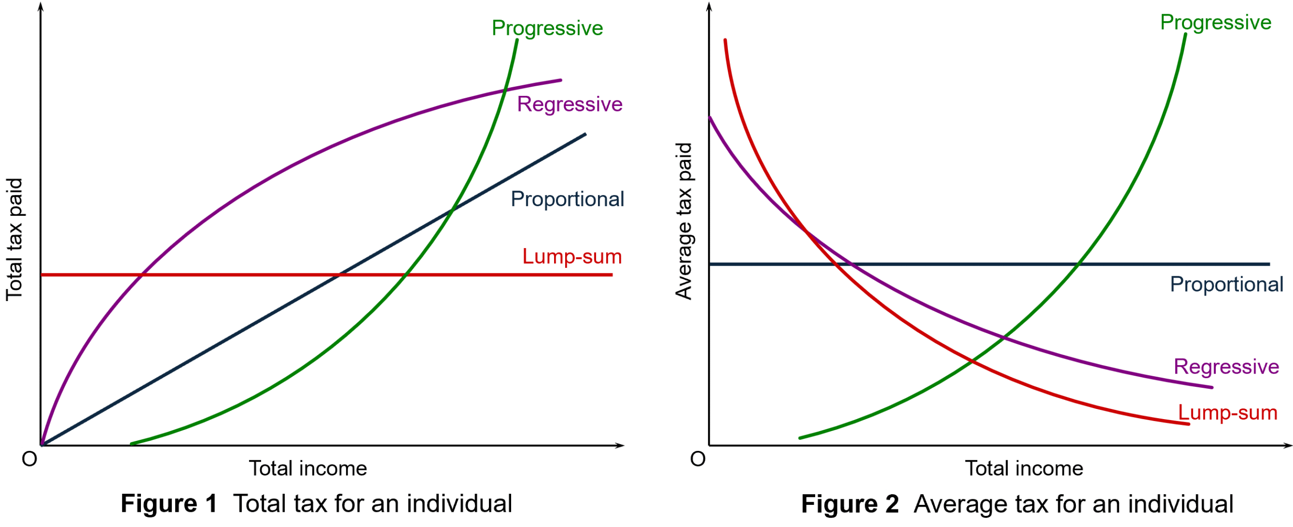
Figures 1 and 2 illustrate these different categories of tax: see Figure 11.12 in Economics, 12th edition. (Click here for a PowerPoint.) Income taxes in most countries are progressive, although just how progressive depends on the differences between the tax bands and the size of personal tax-free allowances. A flat-rate income tax with no allowances is shown by the black line in each diagram, the slope in Figure 1 and the height in Figure 2 depending on the tax rate.
Arguments for a flat-rate income tax
Generally, arguments in favour of flat-rate taxes come from the political right. The two main arguments in favour are tax simplification and incentives.
Advocates argue that a flat tax system makes tax collection easier and makes tax evasion harder. If there are no exemptions, then it can be easier to check that people are paying their taxes and working out the correct amount they owe. It is argued that, in contrast, high tax rates on top earners can encourage tax evasion.
Flat taxes can also be part of a drive to reduce the size of the informal economy. As the VoxEU article states:
Unlike progressive taxes, which include complex and numerous exceptions left to the tax collectors’ discretion, the flat tax is clear cut. In combination with the low rate, its simplicity considerably reduces the stimuli for being informal.
Several post-communist countries in Eastern Europe adopted flat taxes, but for most they were seen as a temporary measure to reduce the informal sector and clamp down on tax evasion. Most have now adopted progressive taxes, with the exceptions of Bulgaria and until recently Russia.
 The second major argument is that lower taxes for higher earners, especially for entrepreneurs, can act as a positive incentive. People work harder and there is more investment. The argument here is that the positive substitution effect from the lower tax (work is more profitable now and hence people substitute work for leisure) is greater than the negative income effect (lower taxes increase take-home pay so that people do not need to work so much now to maintain their standard of living).
Then there is the question of tax evasion. With high rates of income tax for top earners, such people may employ accountants to exploit tax loopholes and hide earnings. This could be seen as highly unfair by middle-income earners who are still paying relatively high rates of tax. Even though a move to flat taxes is likely to mean a cut in tax rates for high earners, the tax take from them could be higher. There is evidence that post-communist and developing countries that have adopted flat taxes have found an increase in tax revenues as evasion is harder.
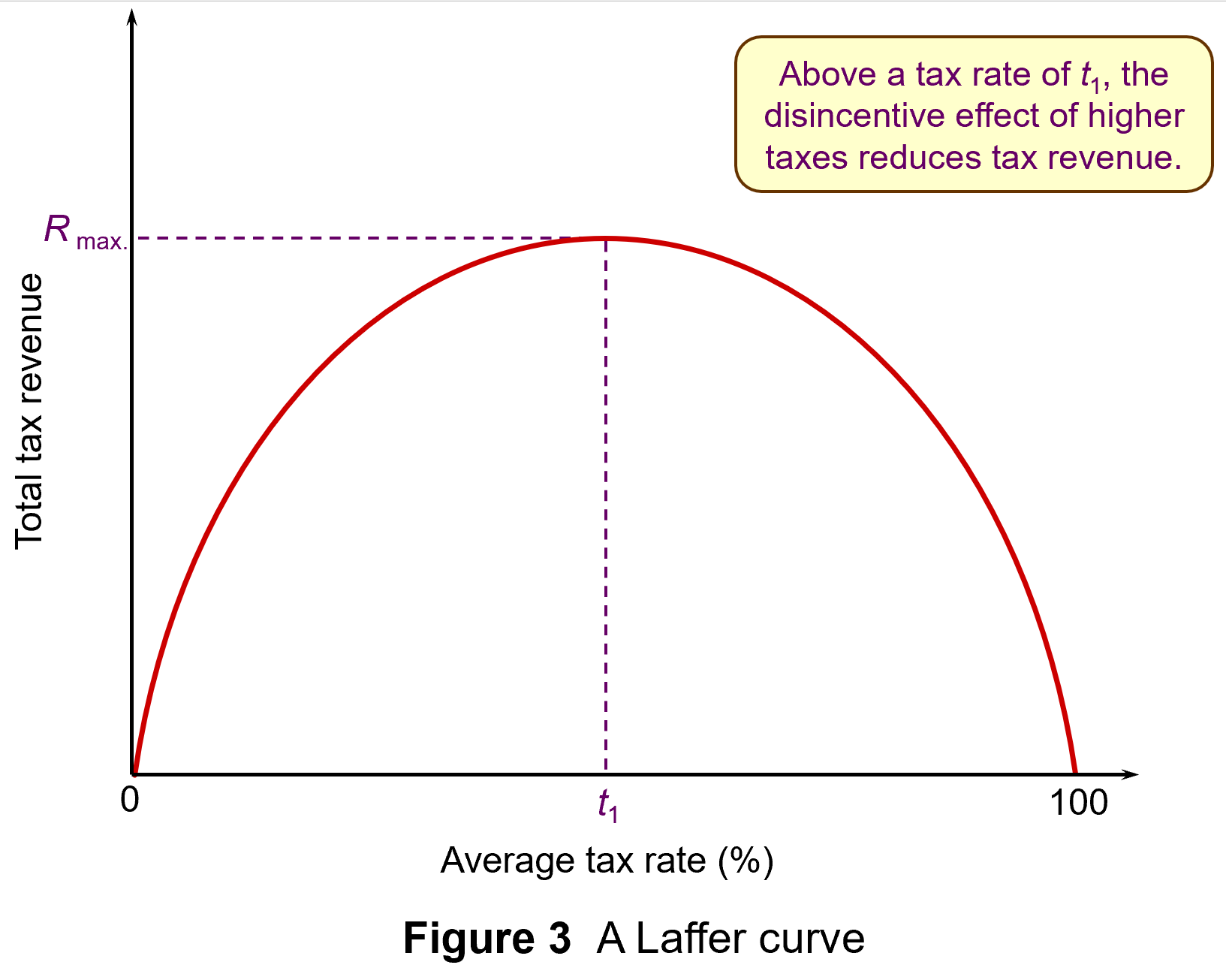 The Laffer curve is often used to illustrate such arguments that high top tax rates can lead to lower tax revenue. Professor Art Laffer was one of President Reagan’s advisers during his first administration (1981–4): see Box 11.3 in Economics, 11th edition. Laffer was a strong advocate of income tax cuts, arguing that substantial increases in output would result and that tax revenues could consequently increase.
The Laffer curve in Figure 3 shows tax revenues increasing as the tax rate increases – but only up to a certain tax rate (t1). Thereafter, tax rates become so high that the resulting fall in output more than offsets the rise in tax rate. When the tax rate reaches 100 per cent, the revenue will once more fall to zero, since no one will bother to work. (Click here for a PowerPoint)
However, as Box 11.3 explains, evidence suggests that tax rates in most countries were well below t1 in the 1980s and certainly are now, given the cuts in income tax rates that have been made around the world over the past 20 years.
Arguments against flat-rate income taxes
 The main argument against moving from a progressive to a flat-rate income tax in an advanced country, such as the UK, is that is would involve a large-scale redistribution of income from the poor to the rich. If the tax were designed to raise the same amount of revenue as at present, those on low incomes would pay more tax than now, as their tax rate would rise to the new flat rate. Those on high incomes would pay less tax, as their marginal rate would fall to the new flat rate.
If a new flat-rate tax in the UK also replaced national insurance contributions (NICs), then the effect would be less extreme as NICs are currently initially progressive, as there is a personal allowance before the 8% rate is applied (on incomes above £12 570 in 2024/25). But above a higher NI threshold (£50 270 in 2024/25), the marginal rate drops to 2%, making it a regressive tax beyond that level. Figure 4 shows tax and NI rates in England, Wales and Northern Ireland for 2024/25. (Click here for a PowerPoint.)
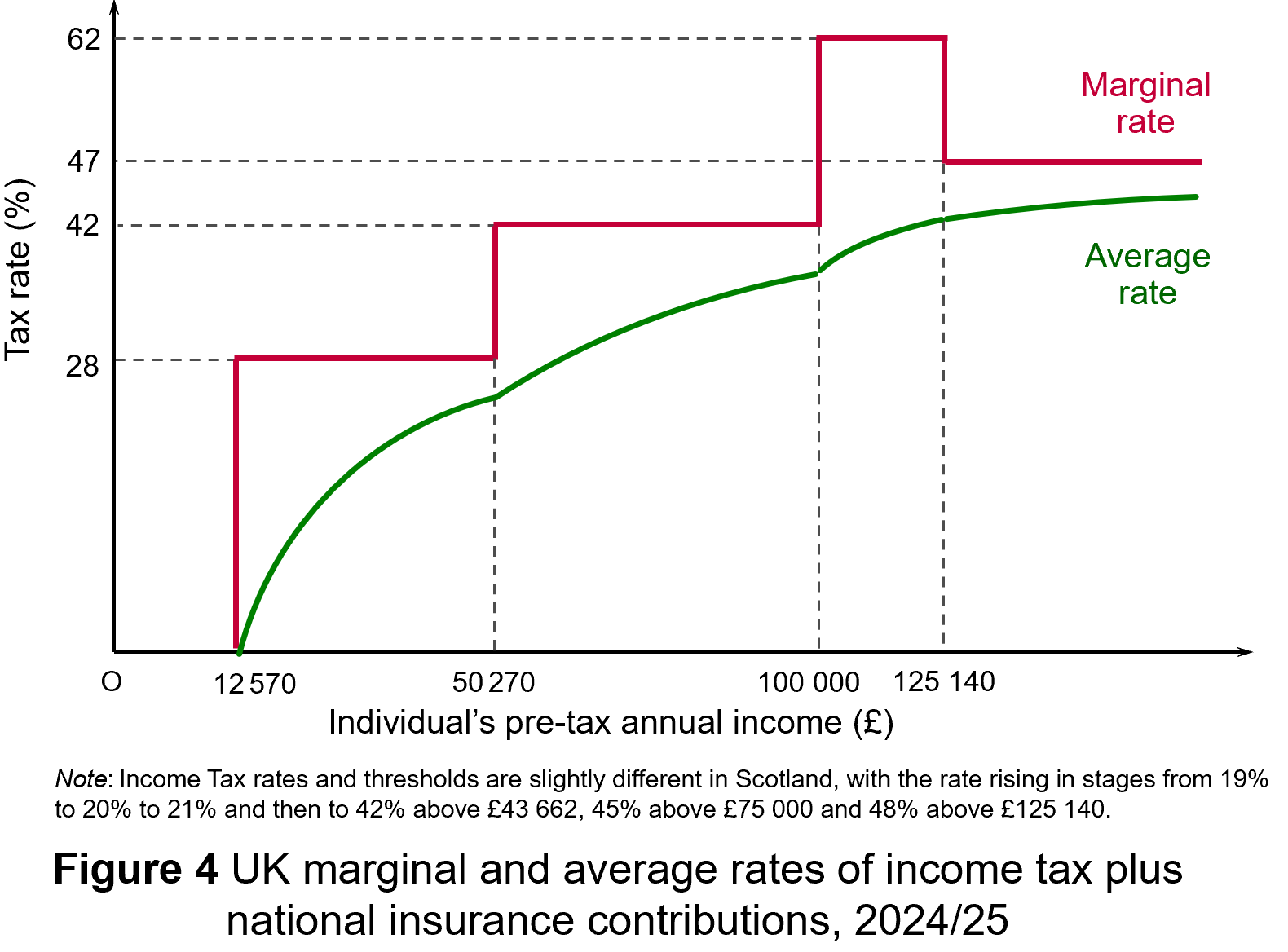 Nevertheless, even if a new flat-rate tax replaced NICs as well as varying rates of income tax, it would still involve a large-scale redistribution from low-income earners to high-income earners. The effect would be mitigated somewhat if personal allowances were raised so that the tax only applied to mid-to-higher incomes. Then the redistribution would be from middle-income earners to high-income earners and also somewhat to low-income earners: i.e. those below, or only a little above, the new higher personal allowance. If, on the other hand, personal allowances were scrapped so that the flat tax applied to all incomes, then there would be a massive redistribution from people on low incomes, including very low incomes, to those on high incomes.
 One of the arguments used to justify a flat-rate tax is that its simplicity would ensure greater compliance. But in an advanced country, compliance is high, except, perhaps, for those on very high incomes. Most people in the UK and many other countries, have tax deducted automatically from their wages. People cannot avoid such taxes.
As far as the self-employed are concerned, they file tax returns online and the software automatically works out the tax due. There are no complex calculations that have to be performed by the individual. There is come scope for tax evasion by charging various expenditures to the business that are really personal spending, but the tax authorities can ask for evidence and sometimes do, with penalties for false claims.
What tax evasion does take place, could still do so with a flat tax. At a rate of, say, 20%, it would still be financially beneficial for a dishonest person to lie if they could get way with it.
Conclusions
If the government did try to introduce a flat-rate income tax, there would probably be an outcry. Also, as some rich people would gain a very large amount of money, the number of people gaining would be lower than the number losing if the total revenue raised were to remain the same. In other words, it would be politically difficult to achieve if the number of losers exceeded the number of gainers.
It is true that if the top rate of income tax were very high, then reducing it might bring in more revenue. But at 45%, or 47% if you include NICs, the top marginal rate in the UK is relatively low compared with other countries. In 2024, the UK had the second lowest top rate of tax out of Western European countries (behind Norway and Switzerland) and only the 16th highest out of 33 European countries when Central and Eastern European countries are also included (see the final ink below under ‘Information’). Reducing the UK’s top rate would be unlikely to bring in more revenue and would redistribute income to high-income earners.
Articles
- Flat tax rate is an ‘attractive idea’, Kemi Badenoch says
The Guardian, Helena Horton (16/12/24)
- Tories could move to a system of ‘flat taxes’ where everyone pays the same rate, Kemi Badenoch indicates
Mail Online, Jason Groves (16/12/24)
- Flat Tax: What It Is and How It Works
Investopedia (8/11/24)
- Flat tax reform in Ukraine: Lessons from Bulgaria
VoxEU, Simeon Djankov (11/12/22)
- Why not… introduce a flat tax?
BBC News, Brian Wheeler (3/7/13)
- Five country cases illustrate how best to improve tax collection
IMF Finance and Development Magazine, Bernardin Akitoby (March 2018)
- Flat taxes and the desire to increase inequality
Funding the Future blog, Richard Murphy (15/5/14)
- Options for a UK ‘flat tax’: some simple simulations
IFS Briefing Note, Stuart Adam and James Browne (August 2006)
- Are the Flat Tax Folks Winning — or Have They Already Won?
Inequality.org, Sam Pizzigati (20/4/24)
Information
Questions
- Distinguish between progressive, proportional, regressive and lump-sum taxes. Into which of these four categories would you place (a) VAT, (b) motor fuel duties, (c) tobacco duties, (d) road-fund licence, (e) inheritance tax? Where the answer is either progressive or regressive, how progressive or regressive are they?
- What are the income and substitution effects of changing tax rates?
- Explain the Laffer curve and consider whether it is likely to be symmetrical.
- Discuss the desirability of having a flat tax set at a relatively high rate (say 25%) with tax-free personal allowances up to the level of income considered to be the poverty threshold. (In the UK the poverty threshold is often defined as 60% of median income.)
- In the London Palladium event where Kemi Badenoch stated that flat taxes were a very attractive idea, she also said that ‘We cannot afford flat taxes where we are now. We need to make sure we rewire our economy so that we can lighten the burden of tax and the regulation on individuals and on those businesses that are just starting out, in particular’. What do you think she meant by this?
- Find out what Bulgaria’s experience of a flat tax of 10% has been.
 On the 29 November, the Bank of England published the results of its latest stress test of the UK financial system. Annual stress testing was introduced in the wake of the 2008 financial crisis. It models the ability of the financial system to withstand severe macroeconomic and financial market conditions. Typically, the focus has been on testing the resilience of the banking system.
This year’s was the first system-wide exploratory scenario (SWES). This recognises the growing significance of ‘shadow banking’. Shadow banking involves borrowing and lending involving non-bank financial institutions (NBFIs). Such institutions sit outside the regulatory cordons around banking but have become significant actors in the financial system.
However, this obscure part of the financial system poses systemic risks which are not clearly understood and from time to time require costly interventions. Examples include: problems in liability-driven investments (LDIs) for pension funds in September 2022; the money market liquidity crisis involving hedge funds in March 2020; the collapse of Long-term Capital Management (LTCM) in 1998 following the Russian Federation’s default (LTCM had significant holdings of Russian government bonds – see linked article on LTCM below).
The growing significance of shadow banking means that regulators have become increasingly concerned about the vulnerabilities in the financial system which arise from outside the traditional banking system.
In this blog we will explain stress-testing of the financial system and trace the rise in shadow banking which motivated the recent system-wide exploratory scenario (SWES). We will discuss the findings of the stress test, highlighting the systemic risks of shadow banking. Finally, we will discuss the implications for the regulation and supervision of the financial system.
What is stress testing?
 Stress testing was introduced by the Bank of England after the financial crisis to assess the ability of the financial system to withstand severe economic and market scenarios.
In the run-up to the 2008 financial crisis, the liquidity and capital buffers of many banks had been extremely thin. These were only able to withstand moderate economic shocks and moderate conditions and buckled under the stresses of the crisis.
Regulators argued that the buffers needed to become much more robust and be able to withstand rare but severe economic and market conditions. The stress testing analogy was derived from engineering, where parts are expected to work not just in benign conditions but also in extreme, hostile environments.
Since 2014, the Bank of England has conducted annual stress testing. Stress testing models the impact of adverse economic conditions on banks’ liquidity, profitability and capital. The results are used to set policy for individual banks (microprudential) and for the system as a whole (macroprudential). Stress test results have allowed the Bank to adjust the loss-absorbing capital that banks must hold to reduce their likelihood of failure.
The scope of the testing has expanded over time to incorporate insurers, central counterparties (financial institutions that provide clearing and settlement services between financial traders) and cyber security. The most recent scenario recognised the increasing significance of non-deposit taking financial institutions in channelling credit. Fifty City of London institutions modelled how a period of intense stress would ripple through the shadow banking sector.
The arcane world of shadow banking
 Shadow banking refers to borrowing and lending which occurs outside the banking sector. Traditionally banking involves taking deposits and using these to finance lending.
Shadow banking involves non-deposit taking financial institutions (NBFIs) such as hedge funds, insurance companies, pension funds, private equity funds, as well as some activities of investment banks. These institutions channel funds in different ways from lenders to borrowers. Typically, they use funds from investors to buy securities through financial markets. The emergence and growth of shadow banking has been explained by changing regulation and innovation.
Its first significant period of expansion in the late 1980s was driven by financial innovation. Increased use of ‘disintermediation’ – the replacement of credit channels through banks with ones through markets – meant an increase in the assets invested through NBFIs.
Despite this process playing a major role in the expansion of housing credit in the run-up to the 2008 financial crisis, it was the significant bailouts that banks received that drew the attention of regulators, not the role of shadow banking. This led to more stringent liquidity and capital requirements for banks under the BASEL III international regulations.
This regulatory tightening limited banks’ ability to offer credit, which meant that much of this activity migrated to the shadow banking sector.
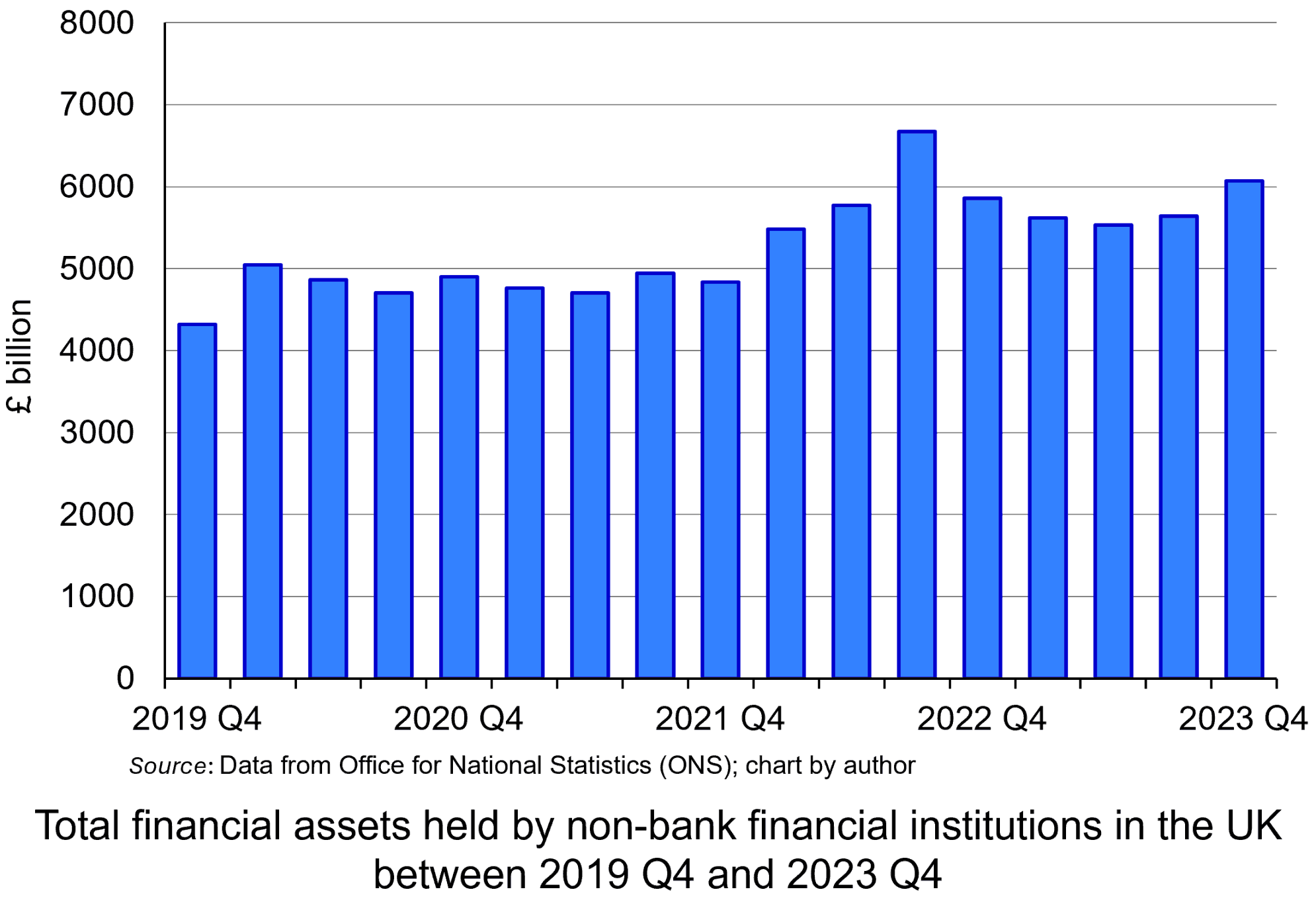 Data from the Bank of England show that the percentage of total assets held by NBFIs rose from 41% in 2007 to 49% in 2020. The chart illustrates the total financial assets held by non-bank financial institutions in the UK between 2019 Q4 and 2023 Q3 (click here for a PowerPoint). The amount held has growth by approximately a third in that time, from £4321bn to £6069bn, peaking at £6670bn in 2022 Q3.
The lack of regulatory oversight stems from the nature of the activities in the shadow banking sector. While NBFIs conduct maturity transformation, provide liquidity and help manage risk, unlike banks, they do not accept deposits and are not part of the payments system involving the general public.
Consequently, the consensus among regulators has been that their activities do not pose the same systemic risks as banking of the breakdown of the payments mechanism and associated collapse in business and consumer confidence. Therefore, NBFIs are not subject to conventional regulation and supervision involving liquidity and capital requirements.
However, as the scale of borrowing and lending running through the sector has grown, this argument has become less difficult to justify. There is a concern that ‘regulatory arbitrage’ is happening and that the systemic risks associated with shadow banking are being underestimated.
The familiar risks of shadow banking
 The systemic consequences of liquidity and solvency problems in the shadow banking sector may not seem obvious. Much of their activities are arcane and technical. However, there are plenty of examples of instances where the problems of hedge funds or pension funds have caused systemic issues.
While the consequences are not the same as those involving banks, in that the payments mechanism is not directly affected, the risks are. Just like banks, these institutions are exposed to liquidity risks, credit default risks and counterparty risks. The concern is that they do not have the same levels of liquidity or capital buffers as banks to insulate them from the consequences of such risks. Therefore, it might not take much economic stress for one or more of these institutions to fail and, given the increasing significance and interconnectedness of these activities, impose significant costs on the rest of the financial system.
It was for this reason that the Bank of England conducted its first system-wide exploratory scenario to analyse the impact of economic and market stress on these institutions and assess the nature and extent of systemic risks which resulted. Fifty City of London institutions modelled how a period of intense stress would ripple through the non-bank sector.
The scenario involved rising geopolitical tensions which caused a sharp rise in risk aversion and a demand for higher expected rates of return as compensation. This produced sharp rises in both sovereign and corporate bond yields and matching sharp declines in asset prices (remember bond yield and prices have a negative relationship).
The scenario found that the position and behaviour of NBFIs amplified the shock. These institutions invest significantly in marketable financial securities and their liquidity and solvency are susceptible to such falling prices.
The sharp decline in asset prices triggered margin calls – payments to cover open loss positions in financial securities. In response to these demands, while some NBFIs’ internal risk and leverage measures were breached, others illustrated greater risk-aversion and took precautionary action. These institutions acted to deleverage, derisk and recapitalise. Given the interconnectedness of financial markets, the individual actions of institutions rippled across financial markets, causing problems in other segments.
The significant decline in asset prices led insurance companies and pension funds to seek to improve their liquidity and solvency position by liquidating positions in money market funds and hedge funds. This, in turn, required these funds to seek liquidity. Such institutions tend to rely a lot on the repo market (involving short-term sale and repurchase credit agreements) to provide liquidity to investors. This avoids them having to sell assets. This practice has echoes of the banking sectors use of the short-term wholesale markets in the run-up to the 2008 financial crisis.
 However, the SWES found that while banks were willing to take on some of the risk, their own concerns about liquidity and counterparty credit risk meant they did not offer sufficient short-term liquidity through the repo markets. If such funding dried up because of a higher risk perception, it could compromise the hedge funds’ ability to raise funds, requiring asset sales. This would amplify the shock to financial markets, driving prices of financial securities even lower.
The scenario concluded that the resulting heavy selling could seize up financial markets, particularly the UK sovereign and corporate bond markets, reducing the ability of companies to finance investment. This is a different type of credit crunch from 2008, which was restricted to banks – but a credit crunch, nonetheless.
At the same time, funds may make capital losses as they sell securities in the downturn. This creates solvency problems and the potential for failure.
In the SWES the institutions were often not able to anticipate how their counterparties, investors, or markets they operate in would behave in the stressed scenario, which echoes the experience of banks in 2007 and 2008 – a significant reason for the ‘crunch’ in banking credit was uncertainty about the creditworthiness of counterparties, meaning that banks were not prepared to lend to anybody.
Conclusion
Since the 2008 financial crisis, there has been a tightening of the regulation and supervision of banks which has limited their ability to channel credit. This has produced an expansion in the shadow banking sector.
However, while the shadow banking sector has not been subject to the same regulation and supervision as banks, there are still potential systemic risks associated with its operations. There have been several examples of such risks in the shadow banking sector which have led regulators to pay more attention. These underpinned the 2024 system-wide exploratory scenario (SWES) conducted by the Bank of England.
The scenario showed the possible transmission mechanism through which problems for NBFIs can have broader consequences. The report nevertheless concluded that:
…the UK financial system was well-capitalised, maintained high levels of liquidity and that asset quality remained strong.
Therefore, the UK financial system was resilient enough to withstand problems in shadow banking.
Although the results of the exercise provide a ‘framework of future system-wide analysis which can be embedded in future market-wide surveillance,’ history indicates that risks tend to exist in obscure and arcane parts of the financial system and that these never tend to be fully appreciated until a crisis occurs. This then tends to involve significant costs for taxpayers.
Articles
- Bank of England warns of risks from non-banks in future markets crisis
Financial Times from MSN, Martin Arnold (29/11/24)
- BoE finds non-bank financial firms pose wider risks in crisis periods
Reuters, Lawrence White (2/12/24)
- Finance Firms Beyond Banks Not Ready For Crisis, BOE Warns
Bloomberg from Yahoo finance, Laura Noonan and Greg Ritchie (29/11/24)
- Shadow Banking System: Definition, Examples, and How It Works
Investopedia, Michael Bromberg (18/10/24)
- US Treasuries: the lessons from March’s market meltdown
Financial Times, Colby Smith and Robin Wigglesworth (29/7/20)
- LDI: the better mousetrap that almost broke the UK
FT Alphaville, Alexandra Scaggs and Louis Ashworth (29/9/22)
- Long-Term Capital Management
CFA Institute, Ron Rimkus (18/4/16)
- Neil Woodford: the continuing fallout of a scandal
Financial Times, Owen Walker (19/3/21)
Bank of England documents and reports
Data
Questions
- Explain stress testing.
- What is shadow banking? Explain the factors driving the growth of credit in this part of the financial system.
- Compare and contrast the liquidity problems of banks with those of non-bank financial institutions (NBFIs).
- Analyse how financial crises can heighten problems of asymmetric information in financial markets.
 In this blog we show how we can apply fiscal metrics to assess the UK government’s fiscal stance. This captures the extent to which fiscal policy contributes to the level of economic activity in the economy.
Changes in the fiscal stance can then be used to estimate the extent to which discretionary fiscal policy measures represent a tightening or loosening of policy. We can measure the size and direction of fiscal impulses arising from changes in the government’s budgetary position.
Such an analysis is timely given the Autumn Budget presented by Rachel Reeves on 30 October 2024. This was the first Labour budget in 14 years and the first ever to be presented by a female Chancellor of the Exchequer.
We conclude by considering the forecast profile of expenditures and revenues for the next few years and the new fiscal rules announced by the Chancellor.
The fiscal stance
At its most simple, the fiscal stance measures the extent to which fiscal policy increases or decreases demand, thereby influencing growth and inflation (see Box 1.F, page 28, Autumn Budget 2024: see link below).
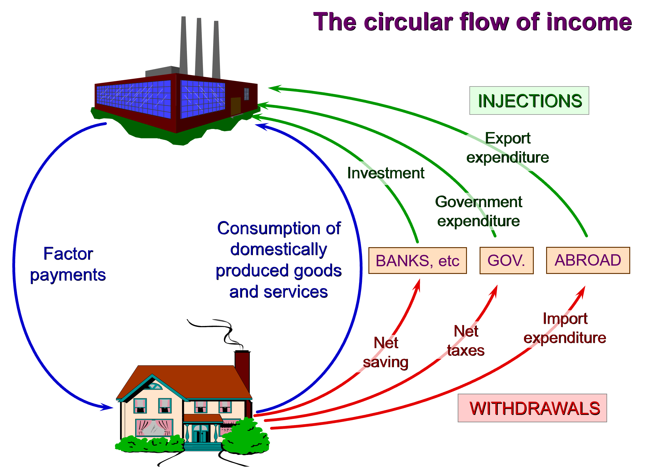 The fiscal stance is commonly estimated by measures of pubic-sector borrowing. To understand this, we can refer to the circular flow of income model. In this model, excesses of government spending (an injection) over taxation receipts (a withdrawal or leakage) represent a net injection into the circular flow and hence positively affect the level of aggregate demand for national output, all other things being equal.
A commonly used measure of borrowing in assessing the fiscal stance of the is the primary deficit. Unlike public-sector net borrowing, which is simply the excess of the sector’s spending over its receipts (largely taxation), the primary deficit subtracts net interest costs. It therefore excludes the interest payments on outstanding public-sector debts (and interest income earned on financial assets). The primary deficit can therefore be written as public-sector borrowing less net interest payments.
As discussed in our blog Fiscal impulses in November 2023, the primary deficit captures whether the public sector is able to afford its present fiscal choices by abstracting from debt-serving costs that reflect past fiscal choices. In this way, the primary deficit is a preferable measure to net borrowing both in assessing the impact on economic activity, i.e. the fiscal stance, and in assessing whether today’s fiscal choices will require government to issue additional debt.
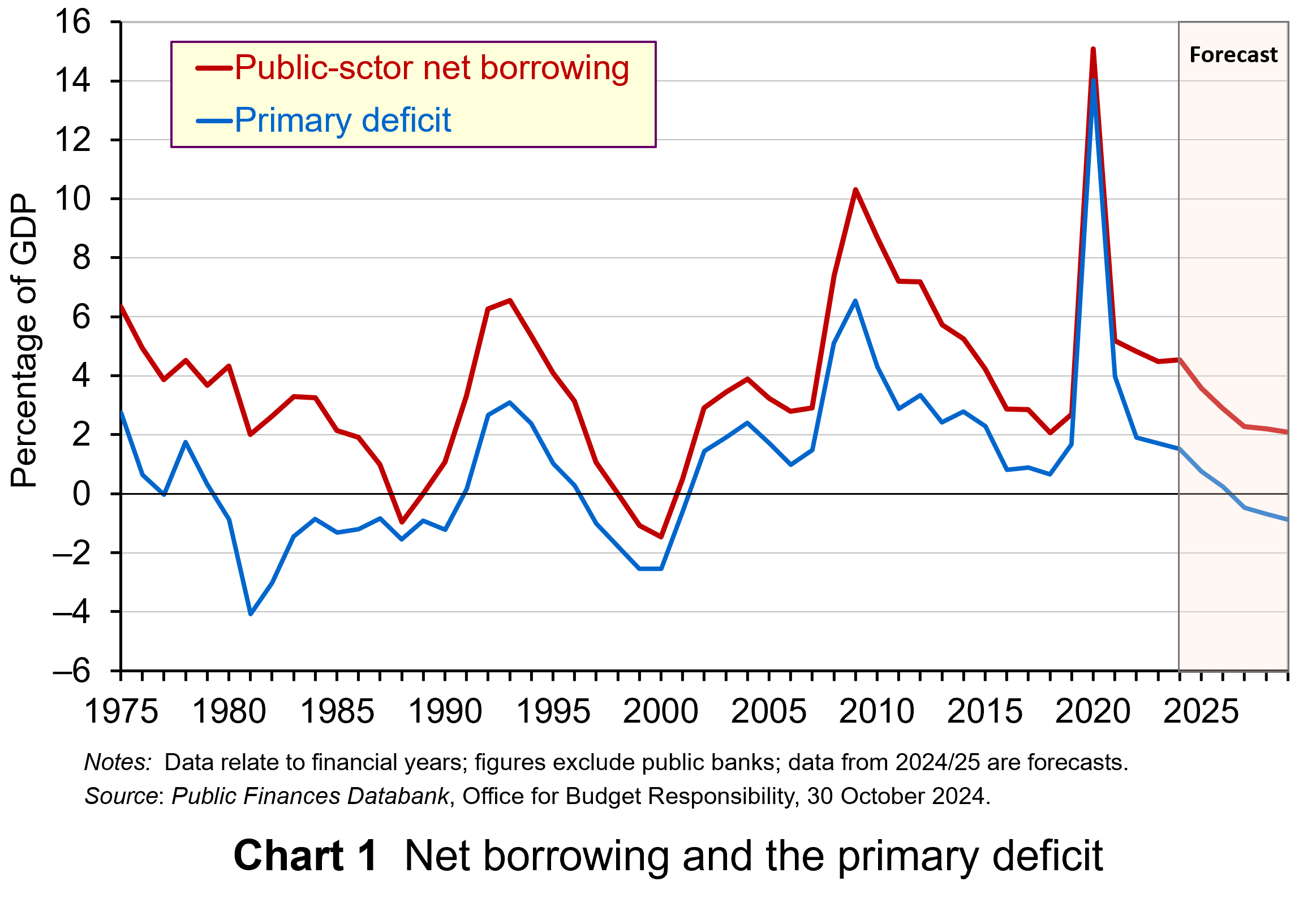 Chart 1 shows public-sector net borrowing and the primary balance as shares of GDP for the UK since financial year 1975/76 (click here for a PowerPoint). The data are from the latest Public Finances Databank published by the Office for Budget Responsibility, published on the day of the Autumn Budget in October (see Data links below).
Over the period 1975/6 to 2023/24, public-sector net borrowing and the primary deficit had averaged 3.8% and 1.3% of GDP respectively. In the financial year 2023/24, they were 4.5% and 1.5% (they had been as high as 15.1% and 14.1% in 2020/21 as a result of COVID support measures). In 2024/25 net borrowing and the primary deficit are forecast to be 4.5% and 1.6% respectively. By 2027/28, while net borrowing is forecast to be 2.3% of GDP, there is forecast to be a primary surplus of 0.7% of GDP.
The Autumn Budget lays out plans for higher tax revenues to contribute two-thirds of the overall reduction in the primary deficit over the forecast period (up to 2029/30), while spending decisions contribute the remaining third.
The largest tax-raising measure is an increase in the employer rate of National Insurance Contributions (NICs) by 1.2 percentage points to 15% from April 2025. This will be levied on employee wages above a Secondary Threshold of £5000, reduced from £9100, which will increase in line with CPI inflation each year from April 2028. (See John’s blog, Raising the minimum wage: its effects on poverty and employment, for an analysis on the effects of this change.) This measure, allowing for other changes to the operation of employer NICs, is expected to raise £122 billion over the forecast period. This amounts to over two-thirds of the additional tax take from the taxation measures taken in the Budget.
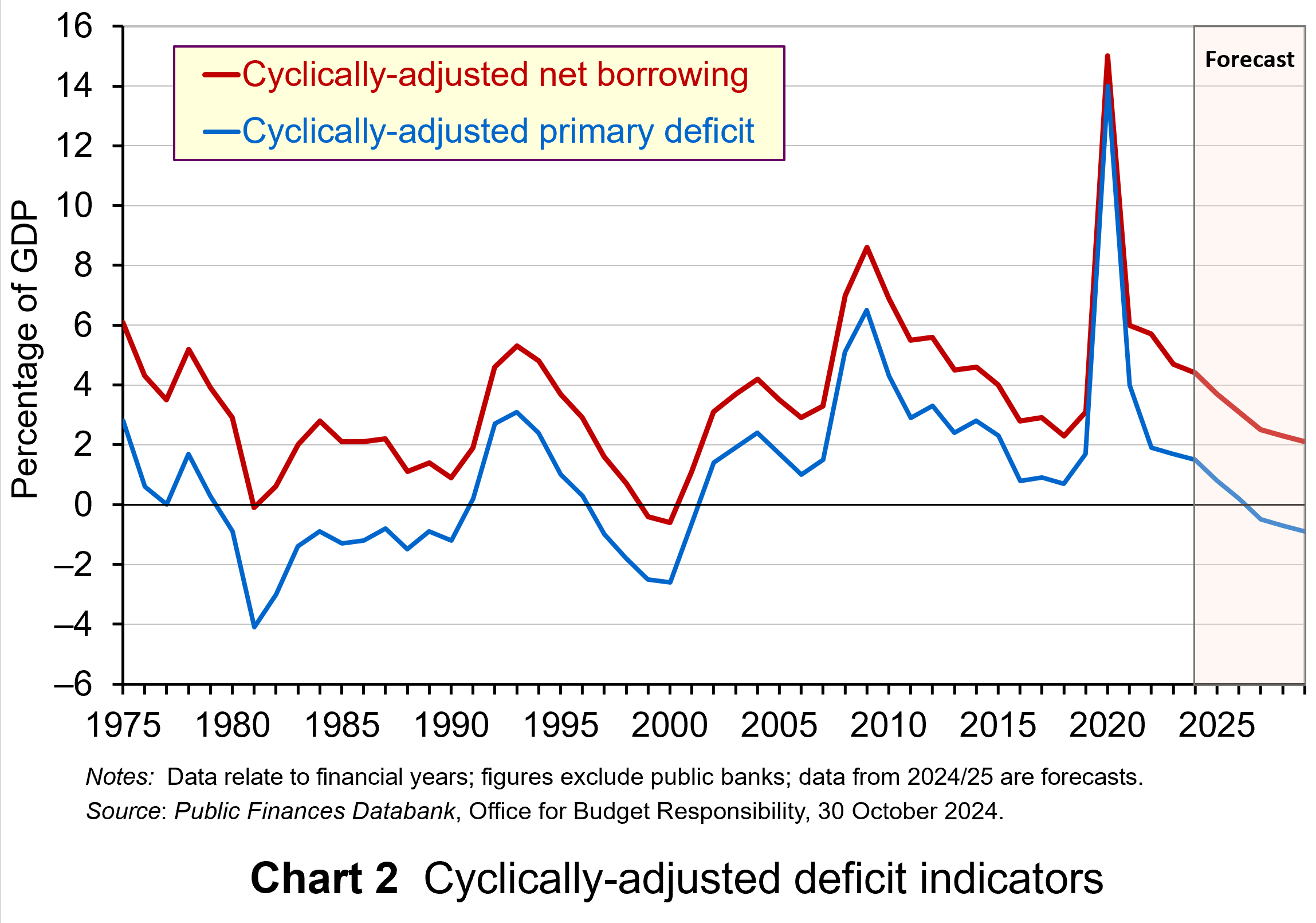 Chart 2 shows both net borrowing and the primary deficit after being cyclically-adjusted (click here for a PowerPoint). This process adjusts these fiscal indicators to account for those parts of spending and taxation that are affected by the position of the economy in the business cycle. These are those parts that act as automatic stabilisers helping, as the name suggests, to stabilise the economy.
The process of cyclical adjustment leads to estimates of receipts and expenditures as if the economy were operating at its potential output level and hence with no output gap. The act of cyclically adjusting the primary deficit, which is our preferred measure of the fiscal stance, allows us to assess better the public sector’s fiscal stance.
Over the period from 1975/6 up to and including 2023/24, the cyclically-adjusted primary deficit (CAPD) averaged 1.1% of GDP. In 2024/25 the CAPD is forecast to be 1.5% of GDP. It then moves to a surplus of 0.5% by 2027/28. It therefore mirrors the path of the unadjusted primary deficit.
Measuring the fiscal impulse
To assess even more clearly the extent to which the fiscal stance is changing, we can use the cyclically-adjusted primary deficit to measure a fiscal impulse. This captures the magnitude of change in discretionary fiscal policy.
The term should not be confused with fiscal multipliers which measure the impact of fiscal changes on outcomes, such as real GDP and employment. Instead, we are interested in the size of the impulse that the economy is being subject to. Specifically, we are measuring discretionary fiscal policy changes that result in structural changes in the government budget and which, therefore, allow an assessment of how much, if at all, a country’s fiscal stance has tightened or loosened.
The size of the fiscal impulse is measured by the year-on-year percentage point change in the cyclically-adjusted public-sector primary deficit (CAPD) as a percentage of GDP. A larger deficit or a smaller surplus indicates a fiscal loosening. This is consistent with a positive fiscal impulse. On the other hand, a smaller deficit or a larger surplus indicates a fiscal tightening. This is consistent with a negative fiscal impulse.
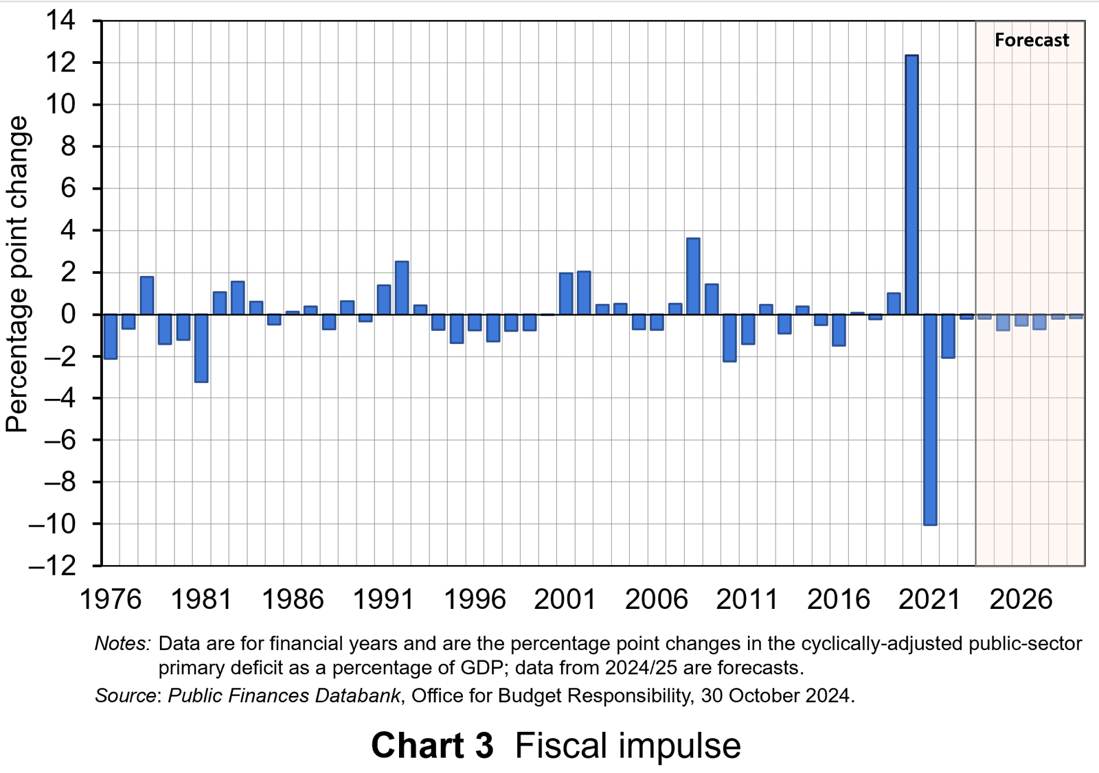 Chart 3 shows the magnitude of UK fiscal impulses since the mid-1970s (Click here for a PowerPoint file). The scale of the fiscal interventions in response to the COVID-19 pandemic, which included the COVID-19 Business Interruption Loan Scheme (CBILS) and Job Retention Scheme (‘furlough’), stand out sharply. In 2020 the CAPD to output ratio rose from 1.7 to 14.4%. This represents a positive fiscal impulse of 12.4% of GDP.
This was followed in 2021 by a tightening of the fiscal stance, with a negative fiscal impulse of 10.1% of GDP as the CAPD to output fell back to 4.0%. Subsequent tightening was tempered by policy measures to limit the impact on the private sector of the cost-of-living crisis, including the Energy Price Guarantee and Energy Bills Support Scheme.
For comparison, the fiscal response to the global financial crisis from 2007 to 2009 saw a cumulative positive fiscal impulse of 5.6% of GDP. While smaller in comparison to the discretionary fiscal responses to the COVID-19 pandemic, it nonetheless represented a sizeable loosening of the fiscal stance.
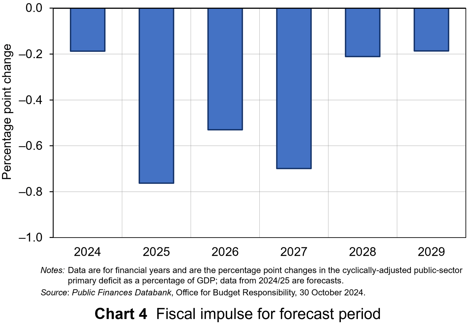 Chart 4 focuses on the implied fiscal impulse for the forecast period up to 2029/30 (click here for a PowerPoint). The period is notable for a negative fiscal impulse each year. Across the period as a whole, this there is a cumulative negative fiscal impulse of 2.6% of GDP. Most of the ‘heavy-lifting’ of the fiscal consolidation occurs in the three financial years from 2025/26 during which there is a cumulative negative impulse of 2.0% of GDP.
Looking forward
To conclude, we consider the implications for the projected profiles of public-sector spending, receipts and liabilities over the forecast period up to 2029/30.
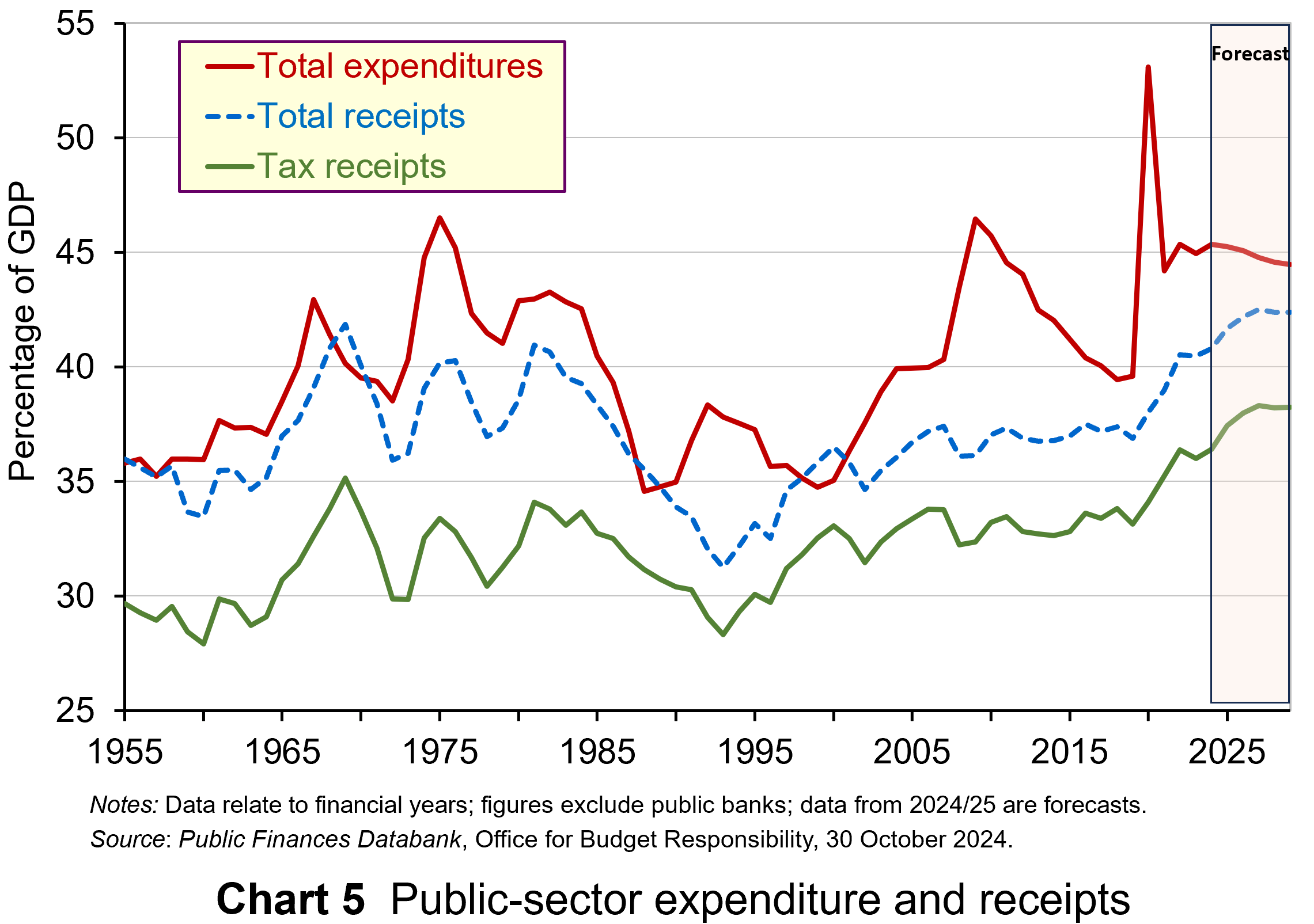 Chart 5 plots data since the mid-1950s (click here for a PowerPoint). It shows the size of total public-sector spending (also known as ‘total managed expenditures’), taxation receipts (sometimes referred as the ‘tax burden’) and total public-sector receipts as shares of GDP. This last one includes additional receipts, such as interest payments on financial assets and income generated by public corporations, as well as taxation receipts.
The OBR forecasts that in real terms (i.e. after adjustment for inflation), public-sector spending will increase on average over the period from 2025/26 to 2029/30 by 1.4% per year, but with total receipts due to rise more quickly at 2.5% per year and taxation receipts by 2.8% per year. The implications of this, as discussed in the OBR’s October 1014 Economic and Fiscal Outlook (see link below), are that:
the size of the state is forecast to settle at 44% of GDP by the end of the decade, almost 5 percentage points higher than before the pandemic” while additional tax revenues will “push the tax take to a historic high of 38% of GDP by 2029-30
Finally, the government has committed to two key rules: a stability rule and an investment rule.
The stability rule. This states that the current budget must be in surplus by 2029/30 or, once 2029/30 becomes the third year of the forecast period, it will be in balance or surplus every third year of the rolling forecast period thereafter. The current budget refers to the difference between receipts and expenditures other than capital expenditures. In effect, it captures the ability of government to meet day-to-day spending and is intended to ensure that over the medium term any borrowing is solely for investment. It is important to note that ‘balance’ is defined in a range of between a deficit and surplus of no more than 0.5% of GDP.
The stability rule replaces the borrowing rule of the previous government that public net borrowing, therefore inclusive of investment expenditures, was not to exceed 3% of GDP by the fifth year of the rolling forecast period.
 The investment rule. The government is planning to increase investment. In order to do this in a financially sustainable way, the investment rule states that public-sector net financial liabilities (PSNFL) or net financial debt for short, is falling as a share GDP by 2029/30, until 2029/30 becomes the third year of the forecast period. PSNFL should then fall by the third year of the rolling forecast period. PSNFL is a broader measure of the sector’s balance sheet than public-sector net debt (PSND), which was targeted under the previous government and which was required to fall by the fifth year of the rolling forecast period.
The new target, as well as now extending to the Bank of England, ‘nets off’ not just liquid assets (i.e. cash in the bank and foreign exchange reserves) but also financial assets such as shares and money owed to it, including expected student loan repayments. While liabilities are broader too, including for example, the local government pension scheme, the impact is expected to reduce the new liabilities target by £236 billion or 8.2 percentage points of GDP in 2024/25. The hope is that both rules can support what the Budget Report labels a ‘step change in investment’.
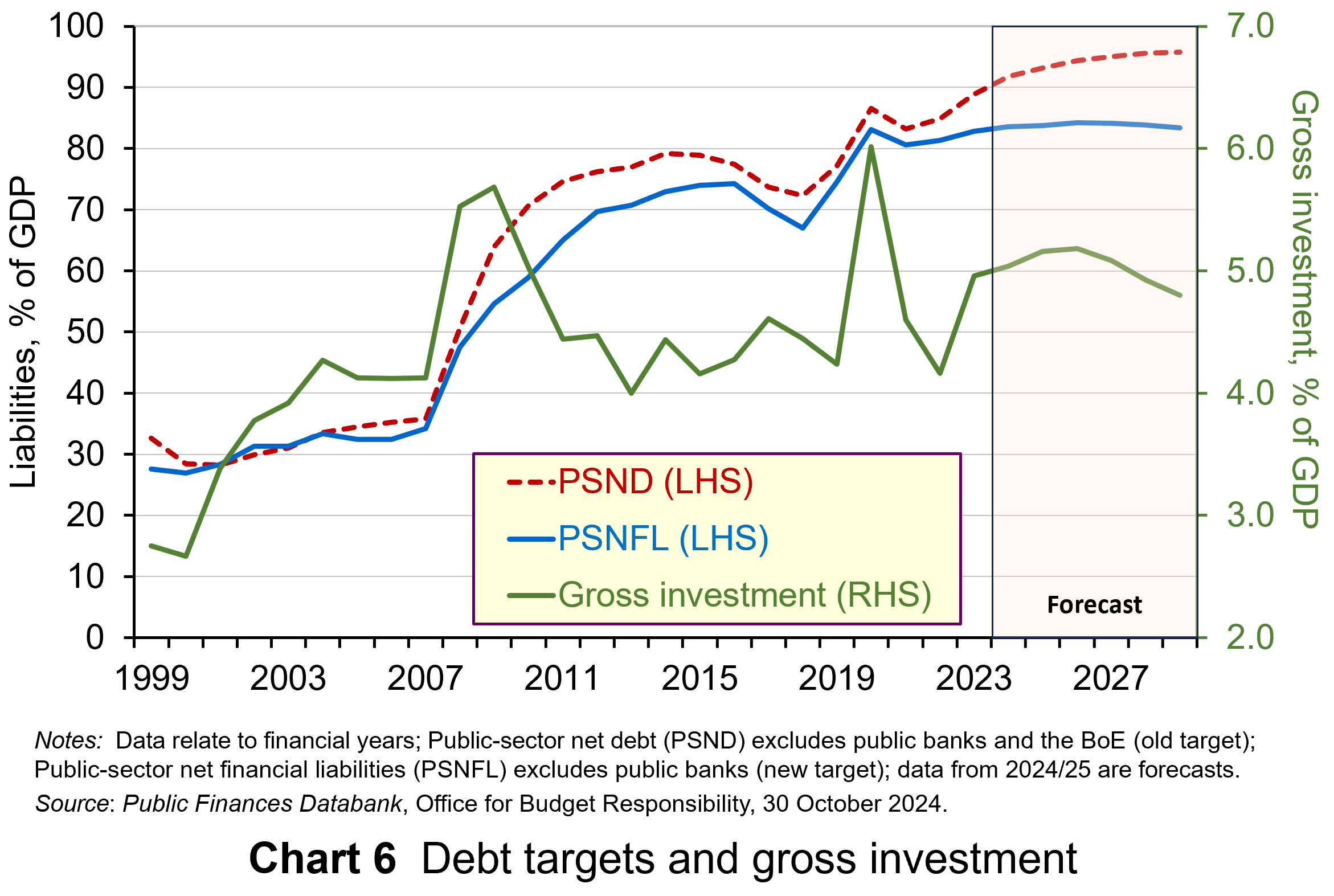 As Chart 6 shows, public investment as a share of GDP has not exceeded 6% this century and during the 2010s averaged only 4.4% (click here for a PowerPoint). The forecast has it rising above 5% for a time, but easing to 4.8% by end of the period.
This suggests more progress will be needed if the UK is to experience a significant and enduring increase in public investment. Of course, this needs to be set in the context of the wider public finances and is illustrative of the choices facing fiscal policymakers across the globe after the often violent shocks that have rocked economies and impacted on the state of the public finances in recent years.
Articles
Official documents
Data
Questions
- Explain what is meant by the following fiscal terms:
(a) Structural deficit,
(b) Automatic stabilisers,
(c) Discretionary fiscal policy,
(d) Public-sector net borrowing,
(e) Primary deficit,
(f) Current budget balance,
(g) Public-sector net financial liabilities (PSNFL).
- Explain the difference between a fiscal impulse and a fiscal multiplier.
- In designing fiscal rules what issues might policymakers need to consider?
- What are key differences between the fiscal rules of the previous Conservative government and the new Labour government in the UK? What economic arguments would you make for and against the ‘old’ and ‘new’ fiscal rules?
- What is meant by the ‘sustainability’ of the public finances? What factors might impact on their sustainability?
 On 25 October 2024, Moody’s, one of the major credit ratings agencies, announced that it was downgrading France’s economic outlook to negative. This was its first downgrading of France since 2012. It followed a similar revision by Fitch’s, another ratings agency, on 11 October.
While Fitch’s announcement did not have a significant impact on the yields of French government bonds, expectations around Moody’s did. In the week preceding the announcement, the net increases in the yield on generic 10-year government debt was approximately 9 basis points (0.09 percentage points). On the day itself, the yield rose by approximately 5.6 basis points (0.056 percentage points).
The yield rose further throughout the rest of October, finishing nearly 0.25 percentage points above its level at the start of the month. However, as Figure 1 illustrates, these increases are part of a longer-term trend of rising yields for French government debt (click here for a PowerPoint).
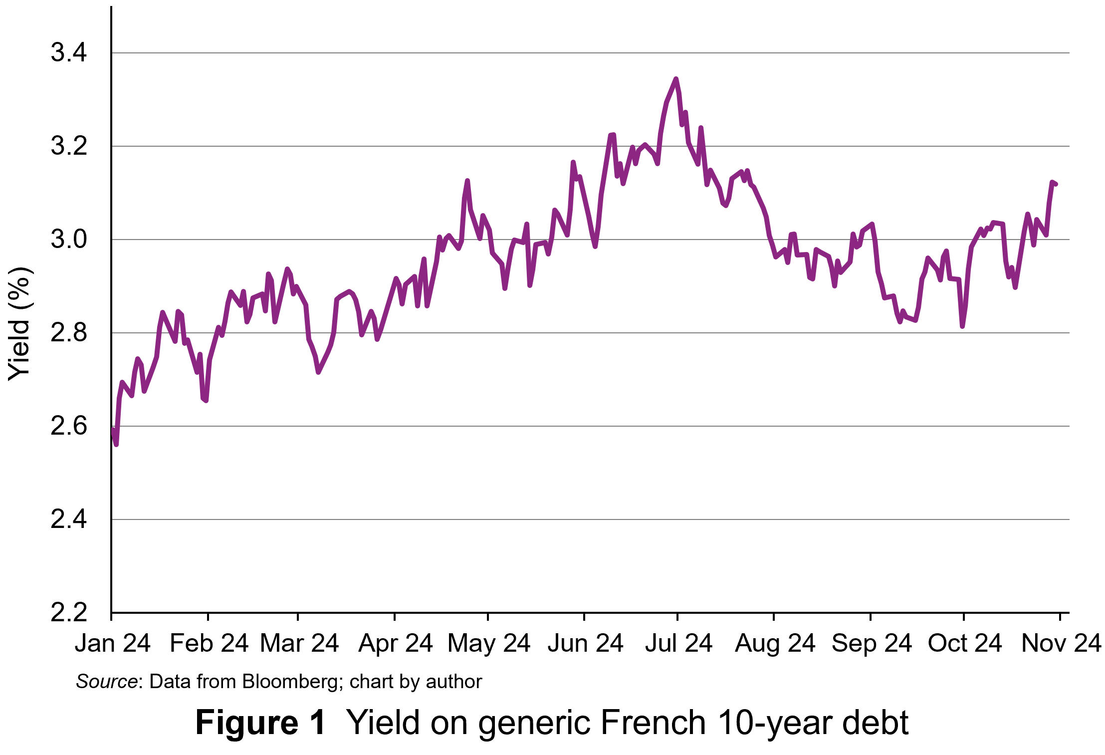 The yield on 10-year French government debt began 2024 at 2.56% and had an upward trend for the first half of the year. The yield peaked at 3.34% on 1 July. It then fell back below 3% for a while. The negative economic outlook then pushed yields back above 3% and they finished October at 3.12%, half a percentage point above the level at the start of the year. This represents a significant increase in borrowing costs for the French government.
In this blog, we will explain why the changes in France’s economic outlook translate into increases in yields for French government bonds. We will also analyse why yields have increased and examine the prospects for the markets in French government bonds.
Pricing signals of bond yields
A bond is a tradable debt instrument issued by governments to finance budget deficits – the difference between tax receipts and spending. Like any financial instruments, investment in bonds involves a commitment of funds today in anticipation of interest payments through time as compensation, with a repayment of its redemption value on the date the bond matures.
Since the cash flows associated with holding a bond occur at different points in time, discounted cash flow analysis is used to determine its value. This gives the present value of the cash flows discounted at the appropriate expected rate of return. In equilibrium this will be equal to the bond’s market price, as the following equation shows.

Where:
P = the equilibrium price of the bond
C = cash coupon payments
M = redemption value at maturity
r = yield (expected rate of return in equilibrium.
Interest payments tend to be fixed at the time a bond is issued and reflect investors’ expected rate of return, expressed as the yield in bond markets. This is determined by prevailing interest rates and perceived risk. Over time, changes in interest rates and perceptions of risk will change the expected rate of return (yield), which will, in turn, change the present value of the cash flows, and hence fundamental value.
Prices move in response to changes in fundamental value and since this happens frequently, this means that prices change a lot. For bonds, as the coupon payments (C each year and the redemption price () are fixed, the only factor that can change is the expected rate of return (yield). This is reflected in the observed yield at each price.
 If the expected rate of return rises, this increases the discount rate applied to future cash flows and reduces their present value. At the current price, the fixed coupon is not sufficient to compensate investors. So, investors sell the bonds and price falls until it reaches a point where the yield offered is equal to that required. The reverse happens if the expected rate of return falls.
The significant risk associated with bonds is credit default risk – the risk that the debt will not be repaid. The potential for credit default is a significant influence of the compensation investors require for holding debt instruments like bonds (ceteris paribus). An increase in expected credit default risk will increase the expected return (compensation). This will be reflected in a lower price and higher yield.
Normally, with the bonds issued by high-income countries, such as those in Europe and North America, the risk of default is extremely low. However, if a country’s annual deficits or accumulated debt increase to what markets consider to be unsustainable levels, the perceived risk of default may rise. Countries’ levels of risk are rated by international ratings agencies, such as Moody’s and Fitch. Investors pay a lot of attention to the information provided by such agencies.
Moody’s downgrade in its economic outlook for France from ‘stable’ to ‘negative’ indicated weak economic performance and higher credit default risk. This revision rippled through bond markets as investors adjusted their views of the country’s economic risk. The rise in yields observed is a signal that bond investors perceive higher credit default risk associated with French government debt and are demanding a higher rates of return as compensation.
Why has France’s credit default risk premium risen now?
As we have seen, credit default risk is not normally considered a significant issue for sovereign borrowers like France. Some of the issue around perceived credit default risk for the French government relate to the size of the French government’s deficit and the projections for it. Following a spike in borrowing associated with the COVID-19 pandemic in 2020, the annual government budget deficit and the overall level of debt as percentages of GDP have remained high. The annual deficit is projected to be 6% for 2024 and still 5% for 2025. The ratio of outstanding French government debt to Gross Domestic Product (GDP) ballooned to 123% in 2020 and is still expected to be 115% by the end of 2025. France has been put on notice to reduce its debt towards the Eurozone limit of 60% of GDP.
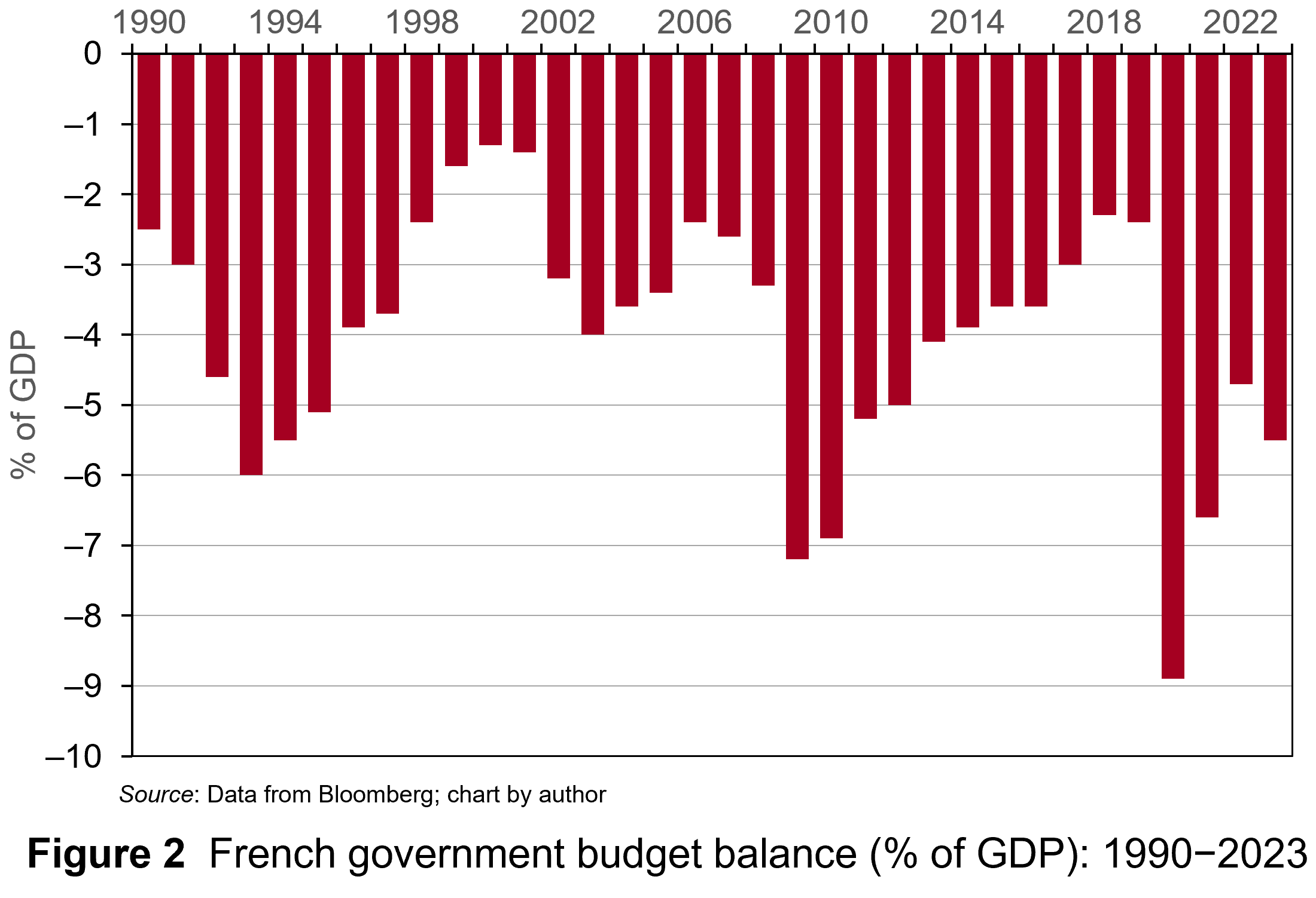 Governments in France last achieved a balanced budget in 1974. They have run deficits ever since. Figure 2 illustrates the French government budget deficits from 1990 to 2023 (click here for a PowerPoint). The figure shows that France experienced deficits in the past similar to today’s. These, however, did not tend to worry bond markets too much.
So why are investors currently worried? This stems from France’s debt mountain and from concerns that the government will not be able to deal with it. Investors are concerned that both weak growth and increasingly volatile politics will thwart efforts to reduce debt levels.
Let’s take growth. Even by contemporary European standards, France’s growth prospects are anaemic. GDP is expected to grow by just 1.1% for 2024 and 1% for 2025. Both consumer and business confidence are low. None of this suggests a growth spurt soon which will boost the tax revenues of the French government sufficiently to address the deficit.
 Further, political instability has grown due to the inconclusive parliamentary elections which Emmanuel Macron surprisingly called in July. No single political grouping has a majority and the President has appointed a Centrist Prime Minister, Michel Barnier (the former EU Brexit negotiator). His government is trying to pass a budget through the Assemblée Nationale involving a mixture of spending cuts and tax hikes which amount to savings of €60 billion ($66 billion). This is equivalent to 2% of GDP.
The parliamentary path of the budget bill is set to be torturous with both the left and right wing blocs in the Assemblée opposing most of the provisions. Debate in the Assemblée Nationale and Senate are expected to drag on into December, with the real prospect that the government may have to use presidential decree to pass the budget. Commentators argue that this will fuel further political chaos.
France looks more like Southern Europe
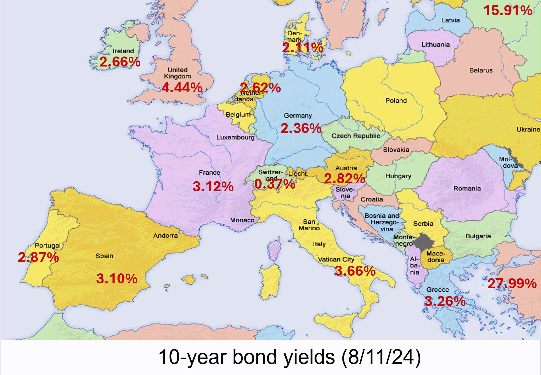 In the past, bond investors were more tolerant of France’s budget deficits. French government bonds were attractive options for investors wanting to hold euro-denominated bonds while avoiding riskier Southern European countries such as Greece, Italy, Portugal and Spain. Since France has run persistent government deficits for a long time, it offered bond investors a more liquid market than more fiscally-parsimonious Northern European neighbours, such as Germany and the Netherlands. Consequently, France’s debt instruments offered a slight risk premium on the yields for those countries.
However, that has changed. France’s credit default risk premium is rising to levels comparable to its Southern neighbours. On 26 September 2024, the yield on generic French government 10-year debt rose above its Spanish equivalent for the first time since 2008.
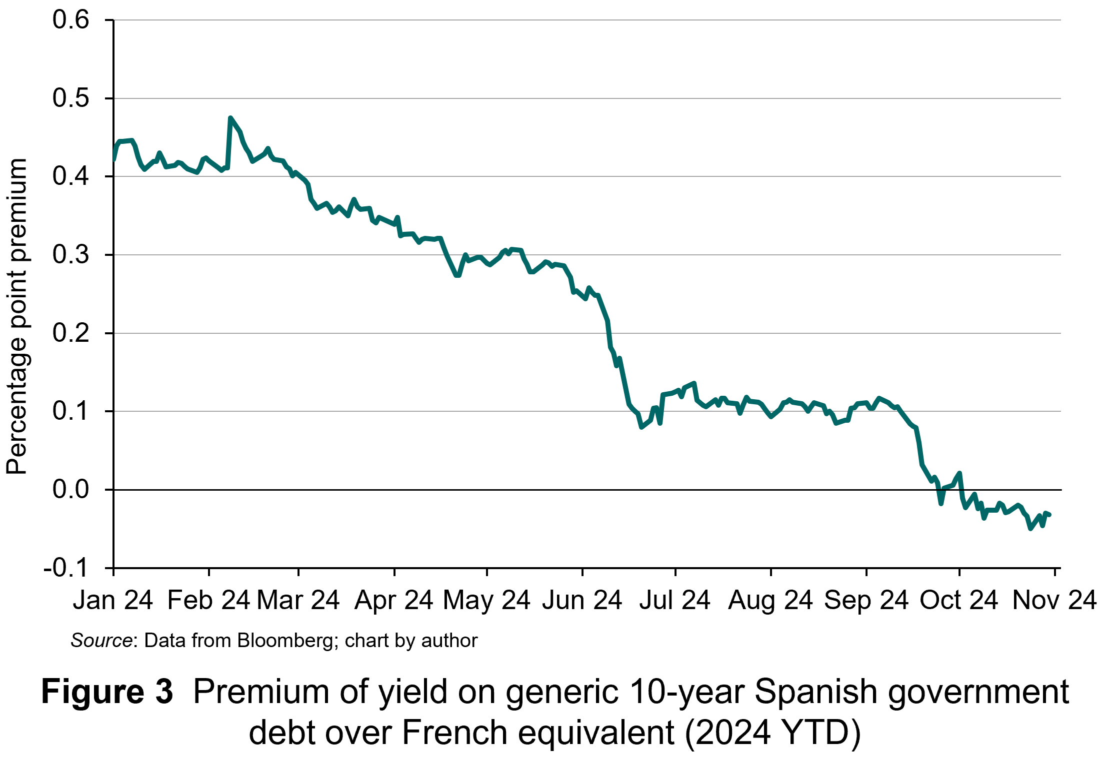 As Figure 3 illustrates, this was the culmination of a trend evident throughout 2024, with the difference in yields between the two declining steadily (click here for a PowerPoint). At the start of the year, the yield on Spanish debt offered a 40 basis points premium over the French equivalent. By October, the yield on Spanish debt was consistently below that of French debt. All of this is due to bond investors’ rising expectations about France’s credit default risk. Now, France’s borrowing costs are not only above Spain, but also closer to those of Greece and Italy than of Germany.
Strikingly, Spain’s budget deficit was 3.5% in 2023 and is expected to narrow to 2.6% by 2025. The percentage of total debt to GDP is 104% and falling. Moreover, following Spain’s inconclusive election in 2023, the caretaker government put forward budgetary plans involving fiscal tightening without the need for legislation. This avoided the political wrangling France is facing.
For France, these developments raise the prospect of yields rising further as bond investors now see alternatives to French government debt in the form of Spain’s. This country have already undertaken the painful fiscal adjustments that France seems incapable of completing.
Articles
Data
Questions
- What is credit default risk?
- Explain why higher credit default risk is associated with higher yields on France’s government debt.
- Why would low economic growth worsen the government’s budget deficit?
- Why would political instability increase credit default risk?
- What has happened to investors’ perceptions of the risk associated with French government debt relative to Spain’s?
- How has this manifested itself in the relative yields of the two countries’ government debt?
 In a blog from March 2023 (reproduced below), we saw how there has been growing pressure around the world for employers to move to a four-day week. Increasing numbers of companies have adopted the model of 80% of the hours for 100% of the pay.
 Since the financial crisis of 2007–8, the growth in UK productivity has been sluggish. This is illustrated in the chart, which looks at the production industries: i.e. it excludes services, where average productivity growth tends to be slower. The chart has been updated to 2024 Q2 – the latest data available. (Click here for a PowerPoint of the chart.)
  Productivity in the UK is lower than in many other competitor countries. According to the ONS, output per hour in the UK in 2021 was $59.14 in the UK. This compares with an average of $64.93 for the G7 countries, $66.75 in France, £68.30 in Germany, $74.84 in the USA, $84.46 in Norway and $128.21 in Ireland. It is lower, however, in Italy ($54.59), Canada ($53.97) and Japan ($47.28).
 The model adopted varied across companies, depending on what was seen as most suitable for them. Some gave everyone Friday off; others let staff choose which day to have off; others let staff work 80% of the hours on a flexible basis.
 At an event at the London Palladium on 6 December staged to protest against elements in the recent Budget, the Conservative leader, Kemi Badenoch, was asked whether she would introduce a flat-rate income tax if the Conservatives were returned to government. She replied that it was a very attractive idea. But first the economy would need ‘rewiring’ so that the tax burden could be lightened.
 The second major argument is that lower taxes for higher earners, especially for entrepreneurs, can act as a positive incentive. People work harder and there is more investment. The argument here is that the positive substitution effect from the lower tax (work is more profitable now and hence people substitute work for leisure) is greater than the negative income effect (lower taxes increase take-home pay so that people do not need to work so much now to maintain their standard of living).
 The Laffer curve is often used to illustrate such arguments that high top tax rates can lead to lower tax revenue. Professor Art Laffer was one of President Reagan’s advisers during his first administration (1981–4): see Box 11.3 in Economics, 11th edition. Laffer was a strong advocate of income tax cuts, arguing that substantial increases in output would result and that tax revenues could consequently increase.
  The main argument against moving from a progressive to a flat-rate income tax in an advanced country, such as the UK, is that is would involve a large-scale redistribution of income from the poor to the rich. If the tax were designed to raise the same amount of revenue as at present, those on low incomes would pay more tax than now, as their tax rate would rise to the new flat rate. Those on high incomes would pay less tax, as their marginal rate would fall to the new flat rate.
 Nevertheless, even if a new flat-rate tax replaced NICs as well as varying rates of income tax, it would still involve a large-scale redistribution from low-income earners to high-income earners. The effect would be mitigated somewhat if personal allowances were raised so that the tax only applied to mid-to-higher incomes. Then the redistribution would be from middle-income earners to high-income earners and also somewhat to low-income earners: i.e. those below, or only a little above, the new higher personal allowance. If, on the other hand, personal allowances were scrapped so that the flat tax applied to all incomes, then there would be a massive redistribution from people on low incomes, including very low incomes, to those on high incomes.
 One of the arguments used to justify a flat-rate tax is that its simplicity would ensure greater compliance. But in an advanced country, compliance is high, except, perhaps, for those on very high incomes. Most people in the UK and many other countries, have tax deducted automatically from their wages. People cannot avoid such taxes.
 On the 29 November, the Bank of England published the results of its latest stress test of the UK financial system. Annual stress testing was introduced in the wake of the 2008 financial crisis. It models the ability of the financial system to withstand severe macroeconomic and financial market conditions. Typically, the focus has been on testing the resilience of the banking system.
 Stress testing was introduced by the Bank of England after the financial crisis to assess the ability of the financial system to withstand severe economic and market scenarios.
 Shadow banking refers to borrowing and lending which occurs outside the banking sector. Traditionally banking involves taking deposits and using these to finance lending.
 Data from the Bank of England show that the percentage of total assets held by NBFIs rose from 41% in 2007 to 49% in 2020. The chart illustrates the total financial assets held by non-bank financial institutions in the UK between 2019 Q4 and 2023 Q3 (click
  The systemic consequences of liquidity and solvency problems in the shadow banking sector may not seem obvious. Much of their activities are arcane and technical. However, there are plenty of examples of instances where the problems of hedge funds or pension funds have caused systemic issues.
  However, the SWES found that while banks were willing to take on some of the risk, their own concerns about liquidity and counterparty credit risk meant they did not offer sufficient short-term liquidity through the repo markets. If such funding dried up because of a higher risk perception, it could compromise the hedge funds’ ability to raise funds, requiring asset sales. This would amplify the shock to financial markets, driving prices of financial securities even lower.
 In this blog we show how we can apply fiscal metrics to assess the UK government’s fiscal stance. This captures the extent to which fiscal policy contributes to the level of economic activity in the economy.
 The fiscal stance is commonly estimated by measures of pubic-sector borrowing. To understand this, we can refer to the circular flow of income model. In this model, excesses of government spending (an injection) over taxation receipts (a withdrawal or leakage) represent a net injection into the circular flow and hence positively affect the level of aggregate demand for national output, all other things being equal.
  Chart 1 shows public-sector net borrowing and the primary balance as shares of GDP for the UK since financial year 1975/76 (click
  Chart 2 shows both net borrowing and the primary deficit after being cyclically-adjusted (click
  Chart 3 shows the magnitude of UK fiscal impulses since the mid-1970s (Click
  Chart 4 focuses on the implied fiscal impulse for the forecast period up to 2029/30 (click
  Chart 5 plots data since the mid-1950s (click
  The investment rule. The government is planning to increase investment. In order to do this in a financially sustainable way, the investment rule states that public-sector net financial liabilities (PSNFL) or net financial debt for short, is falling as a share GDP by 2029/30, until 2029/30 becomes the third year of the forecast period. PSNFL should then fall by the third year of the rolling forecast period. PSNFL is a broader measure of the sector’s balance sheet than public-sector net debt (PSND), which was targeted under the previous government and which was required to fall by the fifth year of the rolling forecast period.
  As Chart 6 shows, public investment as a share of GDP has not exceeded 6% this century and during the 2010s averaged only 4.4% (click
  On 25 October 2024, Moody’s, one of the major credit ratings agencies, announced that it was downgrading France’s economic outlook to negative. This was its first downgrading of France since 2012. It followed a similar revision by Fitch’s, another ratings agency, on 11 October.
 The yield on 10-year French government debt began 2024 at 2.56% and had an upward trend for the first half of the year. The yield peaked at 3.34% on 1 July. It then fell back below 3% for a while. The negative economic outlook then pushed yields back above 3% and they finished October at 3.12%, half a percentage point above the level at the start of the year. This represents a significant increase in borrowing costs for the French government.
 If the expected rate of return rises, this increases the discount rate applied to future cash flows and reduces their present value. At the current price, the fixed coupon is not sufficient to compensate investors. So, investors sell the bonds and price falls until it reaches a point where the yield offered is equal to that required. The reverse happens if the expected rate of return falls.
  Governments in France last achieved a balanced budget in 1974. They have run deficits ever since. Figure 2 illustrates the French government budget deficits from 1990 to 2023 (click
  Further, political instability has grown due to the inconclusive parliamentary elections which Emmanuel Macron surprisingly called in July. No single political grouping has a majority and the President has appointed a Centrist Prime Minister, Michel Barnier (the former EU Brexit negotiator). His government is trying to pass a budget through the Assemblée Nationale involving a mixture of spending cuts and tax hikes which amount to savings of €60 billion ($66 billion). This is equivalent to 2% of GDP.
 In the past, bond investors were more tolerant of France’s budget deficits. French government bonds were attractive options for investors wanting to hold euro-denominated bonds while avoiding riskier Southern European countries such as Greece, Italy, Portugal and Spain. Since France has run persistent government deficits for a long time, it offered bond investors a more liquid market than more fiscally-parsimonious Northern European neighbours, such as Germany and the Netherlands. Consequently, France’s debt instruments offered a slight risk premium on the yields for those countries.
  As Figure 3 illustrates, this was the culmination of a trend evident throughout 2024, with the difference in yields between the two declining steadily (click