 At the fourth anniversary of Russia’s invasion of Ukraine, we look at the effect of the war on the Russian economy. Two years ago, in the blog The Russian economy after two years of war, we argued that the Russian economy had seemingly weathered the war successfully.
Unlike Ukraine, very little of its infrastructure had been destroyed; it had started the war with a current account balance of payments surplus, a budget surplus and a low general government debt-to-GDP ratio; it had achieved a lot of success in diverting its exports, including oil, away from countries imposing sanctions to countries such as China and India; it was the same with imports, with China especially becoming a major suppliers of machinery, components and vehicles; it has a strong central bank, which engenders a high level of confidence in managing inflation; the military expenditure provided a Keynesian boost to the economy, with production and employment rising.
The situation today
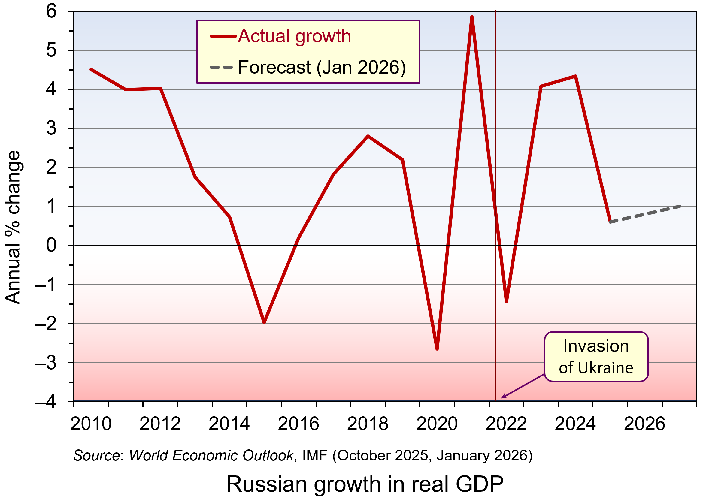 But two years further on, the Russian economy is looking a lot weaker and on the verge of recession. GDP growth fell to 0.6 per cent in 2025 and is forecast to be no more than 1 per cent for the next two years. (Click here for a PowerPoint of the chart.) And despite growth still being positive (just), this is largely because of the growth in military expenditure. Retail and wholesale trade fell by 1.1% in 2025, reflecting supply chain problems and high inflation dampening consumer demand.
With labour being diverted into the armaments and allied industries or into the armed forces, this has led to labour shortages. This has been compounded by the emigration of up to 1 million people by 2025 – often young, educated and skilled professionals.
 Official CPI inflation averaged 8.7 per cent in 2025, although the prices of food and other consumer essentials rose by more, especially in recent months. At the beginning of 2026, supermarket prices rose by 2.3% in just one month, made worse by a rise in VAT from 20% to 22%. The central bank has responded to the high inflation with high interest rates, which averaged 19.2% in 2025, giving a real rate of 10.5%. With such a high real rate, the response of households has been to save. This has masked the constraints on production, or imports, of consumer goods. Savings have also been boosted by large payments to soldiers and bereaved families, with the money saved by the recipients being used in part to fund future such payments. So far there has been trust in the banking system, but if that trust waned and people starting making large withdrawals of savings, it could be seriously destabilising.
Whilst the high real interest rates have helped to mask shortages of consumer goods, they have had a seriously dampening effect on investment by domestic companies. Gross capital formation fell by 3% in 2025, not helped by an increase in the corporation tax from 20% to 25%. At the same time, foreign direct investment remains subdued due to high perceived risks. The lack of investment, plus the labour shortages, will have profound effects on the supply side of the economy, with potential output in the non-military sector likely to decline over the medium term.
 The balance of payments and government finances are turning less favourable. The balance of trade surplus has declined from US$173bn in 2021 to US$67bn in 2025. This could decline further, or even become a deficit, if oil prices continue to be weak, if Western sanctions are tightened (such as stopping the flow of Russian oil exports in the ‘shadow’ fleet of tankers) or if major importing countries stop buying Russian oil. Indian refiners have announced that they are not taking Russian crude in March/April as India seeks to finalise a trade deal with the USA.
The budget balance has moved from a small surplus of 0.8% of GDP in 2021 to a deficit of 2.9% in 2025. Although the government debt-to-GDP ratio remains low by international standards at 23.1% of GDP in 2025, this was up from 16.5% in 2021 and is set to rise further as budget deficits deepen. Nevertheless, as long as the saving rate remains high, the debt can be serviced by domestic bond purchase.
Russia’s economy is definitely weakening and labour shortages and low investment will create major problems for the future. But whether this deterioration will be enough to change Russia’s stance on the war in Ukraine remains to be seen.
Articles
- The Russian economy is finally stagnating. What does it mean for the war – and for Putin?
The Guardian, Alex Clark (6/2/26)
- Exclusive: Russia’s budget deficit may almost triple this year as oil revenues decline
Reuters (4/2/26)
- Russia’s war economy is not collapsing, but neither is it stable
The Conversation, Yerzhan Tokbolat (17/12/25)
- Food prices are surging in Russia. Is the war hitting Russians in the pocket?
BBC News, Olga Shamina, Yaroslava Kiryukhina and Sergei Kagermazov (18/2/26)
- [Russian] GDP data — what it reveals, what it conceals
The Bell, Denis Kasyanchuk (18/2/26)
 What to Expect From the Russian Economy in 2026
Carnegie Endowment for International Peace, Alexandra Prokopenko and Alexander Gabuev (12/2/26)
- Indian refiners avoid Russian oil in push for US trade deal
Reuters, Nidhi Verma (8/2/26)
- What Breaks First – Russia’s Economy or Its War?
Visegrad Insight, Tomasz Kasprowicz (3/2/26)
Videos
Reports
Data
Questions
- What constraints are there currently on the supply side of the Russian economy?
- Some economists have argued that the economic effects of a stalemate in the Ukraine war would suit the Russian leadership more than peace or victory. Why might this be so?
- Under what circumstances might a deep recession in Russia be more likely than stagnation?
- In what ways does Russia’s current financial system resemble a pyramid scheme?
- What cannot a Keynesian boost contunue to support the Russian economy indefinitely?
 The approach towards mergers remains the most controversial area of competition policy. Some argue that policy makers in both the UK and EU have been too easily persuaded by the arguments put forward by firms and so have allowed too many mergers to proceed. Others claim that the opposite is true and that merger policy has prohibited mergers that should have been allowed to proceed. This, then, has a negative impact on investment, innovation, productivity and growth.
In recent years there has been more specific criticism of merger policy in the UK. The government has indicated that it wants the Competition and Markets Authority (CMA) to be less interventionist and take a more pro-growth approach.
 In February 2025, in response to this criticism, the CMA launched its new ‘4 Ps’ approach to merger policy: Pace, Predictability, Proportionality and Process. Various changes to the investigation process have been proposed in the past 12 months using this framework.
Pace. The time taken by the CMA to initially assess a merger before deciding whether a Phase 1 investigation is necessary (i.e. the pre-notification procedure) was reduced from 65 to 40 working days. Also, the target to complete straightforward Phase 1 investigations was reduced from 35 to 25 days.
Predictability. The proposed merger guidelines, published in October 2025, provide more detail on (a) what criteria will be used to measure market shares when applying the ‘share of supply test’ (this is where the combined UK market share of two merging businesses is at least 25%, provided one business has a UK turnover of at least £10 million), and (b) the factors that are likely to lead to the competition authorities concluding that one business has gained ‘material influence over another’. Businesses had complained that there was too much uncertainty about the way the share of supply test and material influence were applied. The CMA is also considering greater alignment with other international regulators over decision making rather than its previous policy of acting independently. All these measures should increase the predictability of the investigation process.
 Proportionality. Proportionality refers to the objective of addressing any competition issues in merger cases in a way that places the minimum burden on the businesses involved. To improve proportionality, the CMA has indicated that in future cases it will be more willing to use behavioural remedies – requiring firms to take or desist from certain actions. New draft guidelines identify more situations where the use of behavioural remedies may be appropriate. However, they also show that the CMA still views structural remedies (e.g. preventing the merger or requiring firms to demerge or to sell certain assets) as more effective in many situations. Another important measure to improve proportionality is the introduction of a new ‘wait and see’ approach to global mergers. The CMA will now wait to see if the actions taken by other competition authorities in global cases address any concerns in the UK market before deciding whether to launch a review.
Process. To improve the process, the CMA has announced plans to engage with businesses at a much earlier point in the process. For example, it has pledged to share its provisional thinking in the early stages of an investigation by implementing new ‘teach-in’ sessions and having more regular update meetings. Much earlier meetings that focus on possible remedies will also take place. This may make it possible for the CMA to assess the suitability of more complex remedies during a Phase 1 investigation rather than having to wait for a longer and more costly Phase 2 review. Phase 2 reviews will also no longer be managed by panels of independent experts. This role will now be carried out by the internal CMA board.
Some critics argue that the CMA has not fully considered the potential benefits of mergers in many cases. For example, a merger could (a) have procompetitive effects, known as rivalry enhancing efficiencies (REEs) and/or (b) benefits for consumers outside of the relevant market, known as relevant customer benefits (RCBs). In response to this criticism, the CMA is currently reassessing its approach to including evidence on REEs and RCBs.
The CMA is still currently consulting with interested parties about many of these proposed changes. It will be interesting to see what final decisions are made in the next couple of years.
Articles
- CMA consults on proposed changes to its merger remedies approach
CMA Press Release (15/10/25)
- New CMA proposals to drive growth, investment and business confidence
CMA Blog, Sarah Cardell (CMA Chief Executive) (13/2/25)
- Promoting competition and protecting consumers to drive growth and improve household prosperity
CMA Speech, Sarah Cardell (20/11/25)
- Steering the course: how the CMA is responding to the Government’s pro-growth agenda
Macfarlanes (21/2/25)
- 4Ps and 3 themes – An overview of the CMA’s merger remedies review
Hogan Lovells, Angus Coulter, Alice Wallace-Wright, Karman Gordon, and Denise Hotham-Kellner (1/4/25)
- CMA publishes updated guidance on UK merger procedure
Ashurst, Christopher Eberhardt, Emile Abdul-Wahab and Finlay Sadler-Wilson (11/11/25)
- Government ousts UK competition watchdog chair
BBC News, Simon Jack and Charlotte Edwards (21/1/25)
- UK competition watchdog drops Microsoft-OpenAI probe
BBC News, Imran Rahman-Jones (5/3/25)
- Does the government really know what it wants from the CMA?
The Guardian, Nils Pratley (13/2/25)
- This article is more than 9 months old ‘We must avoid a chilling effect’: the CMA chief on the UK’s pro-growth shift
The Guardian, John Collingridge (18/2/25)
- The CMA should be nudged on antitrust, not bullied
The Financial Times, John Gapper (6/2/25)
CMA documentation
Questions
- Of all the mergers considered by the CMA in 2024/25, find out what percentage were formally investigated. How many were blocked from taking place? Do you believe that this indicates that merger policy is too weak or too strong?
- What three criteria must be met for a business arrangement to be classed as a ‘relevant merger situation’ by the CMA?
- Identify some different methods that one business could use to gain material influence over the way another company operates.
- Outline the ‘turnover test’, the ‘share of supply test’ and the ‘hybrid test’.
- Discuss the potential advantages of using behavioural remedies as opposed to structural remedies in merger cases. Why has the CMA still preferred the use of structural remedies in most situations?
 The productivity gap between the UK and its main competitors is significant. In 2024, compared to the UK, output per hour worked was 10.0% higher in France, 19.8% higher in Germany and 41.1% higher in the USA. These percentages are in purchasing-power parity terms: in other words, they reflect the purchasing power of the respective currencies – the pound, the euro and the US dollar.
GDP per hour worked (in PPP terms) is normally regarded as the best measure of labour productivity. An alternative measure is GDP per worker, but this does not take into account the length of the working year. Using this measure, the gap with the USA is even higher as workers in the USA work longer hours and have fewer days holiday per year than in the UK.
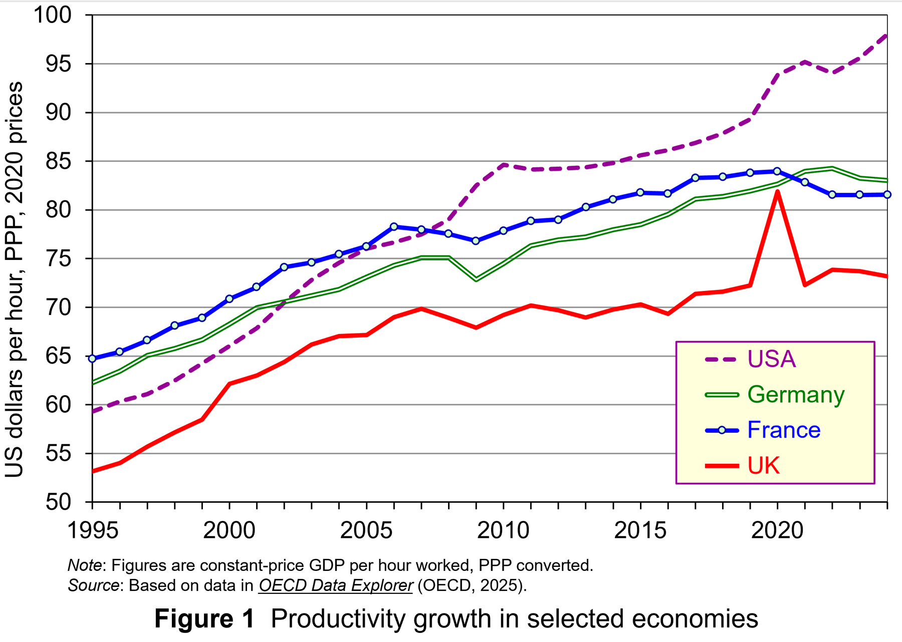 The productivity gap is not a new phenomenon. It has been substantial and growing over the past 20 years. (The exception was in 2020 during lockdowns when many of the least productive sectors, such as hospitality, were forced to close temporarily.)
The productivity gap is shown in the two figures. Both figures show labour productivity for the UK, France, Germany and the USA from 1995 to 2024.
Figure 1 shows output (GDP) per hour, measured in US dollars in PPP terms.
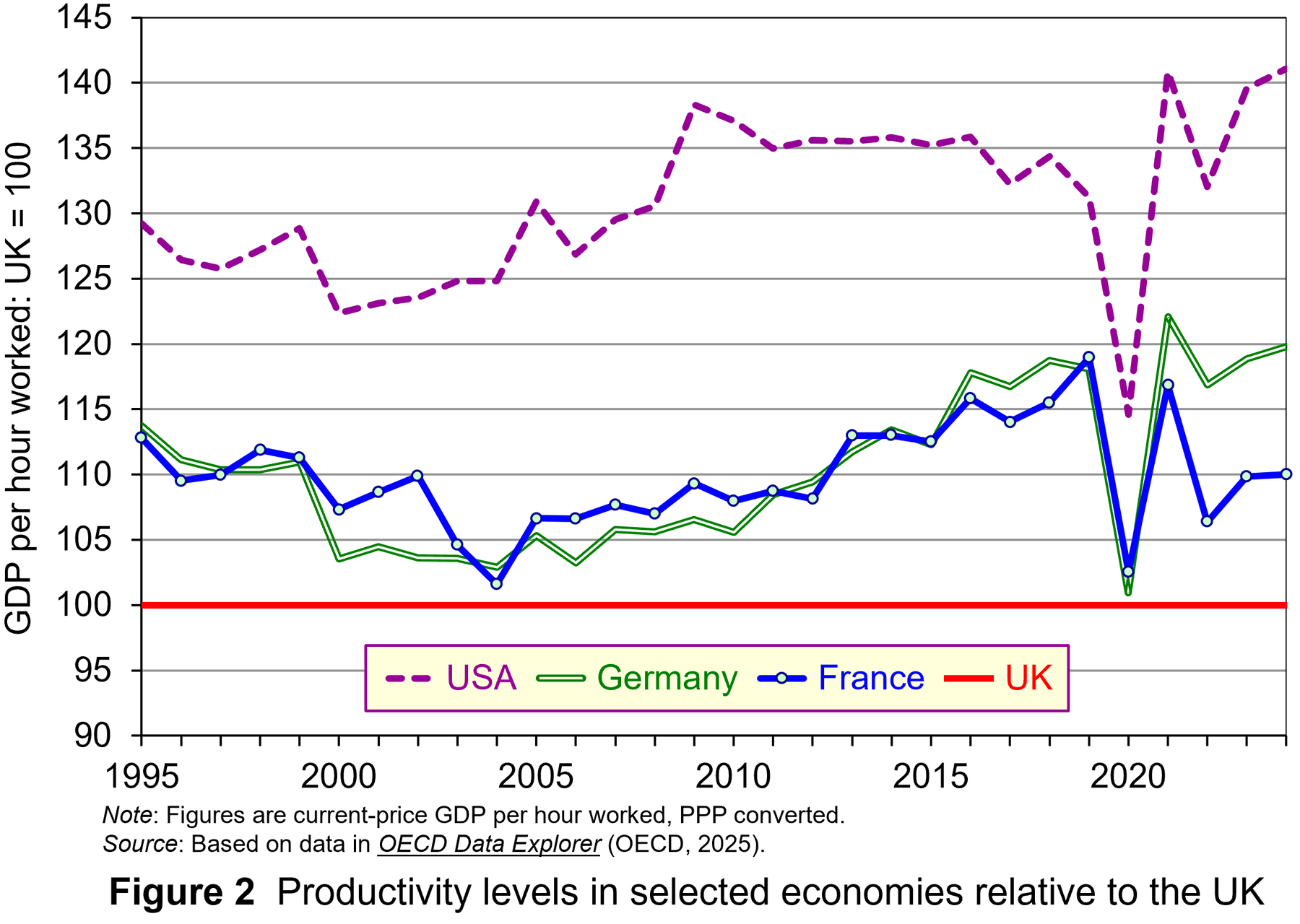 Figure 2 shows output (GDP) per hour relative to the UK, with the UK set at 100. The gap narrowed somewhat up to the early 2000s, but since then has widened.
Low UK productivity has been a source of concern for UK governments and business for many years. Not only does it constrain the growth in living standards, it also make the UK less attractive as a source of inward investment and less competitive internationally.
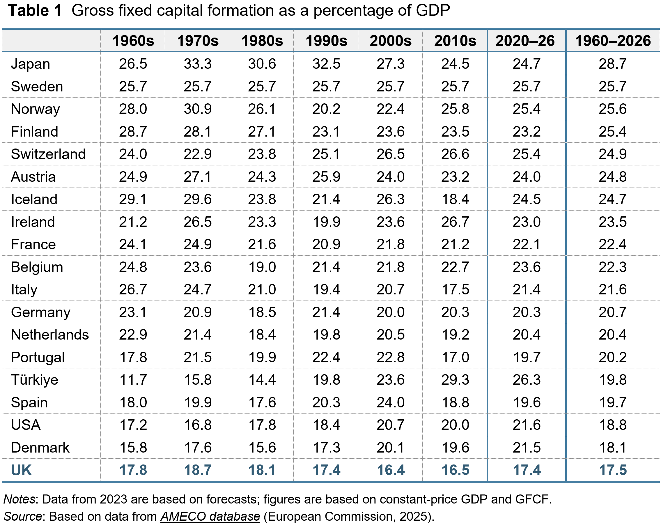
Part of the reason for low UK productivity compared to that in other countries is a low level of investment. As a proportion of GDP, the UK has persistently had the lowest, or almost the lowest, level of investment of its major competitors. This is illustrated in Table 1.
It is generally recognised by government, business and economists that if the economy is to be successful, the productivity gap must be closed. But there is no ‘quick fix’. The policies necessary to achieve increased productivity are long term. There is also a recognition that the productivity problem is a multi-faceted one and that to deal with it requires policy initiatives on a broad front: initiatives that encompass institutional changes as well as adjustments in policy.
So what can be done to improve productivity and how can this be achieved at the micro as well as the macro level?
Improving productivity: things that government can do
 Encouraging investment. Over the years, UK governments have increased investment allowances, enabling firms to offset the cost of investment against pre-tax profit, thereby reducing their tax liability. For example, in the UK, companies can offset a multiple of research and development costs against corporation tax. The rate of relief for small and medium-sized enterprises (SMEs) allows companies that work in science and technology to deduct an extra 86% of their qualifying expenditure from their trading profit in addition to the normal 100% deduction: i.e. a total of 186% deduction. Meanwhile, since April 2016, larger companies have been able to claim a R&D expenditure credit, initially worth 11 per cent of R&D expenditures, then 12 per cent from 2018 and 13 per cent from 2020. This was then raised to 20 per cent from 2023.
Strengthening competition. A number of studies have revealed that, with increasing market share, business productivity growth slows. As a result, government policy sought to strengthen competition policy. The Competition Act 1998, which came into force in March 2000, and the Enterprise Act of 2002, enhanced the powers of the Office of Fair Trading (OFT) (a predecessor to the Competition and Markets Authority) in respect to dealing with anti-competitive practices. It was given the ability to impose large fines on firms which had been found guilty of exploiting a dominant market position. Today, one of the strategic goals of the Competition and Markets Authority (CMA) is the aim of ‘extending competition frontiers’ in order to improve the way competition works.
Encouraging an enterprise culture. The creation of an enterprise culture is seen as a crucial factor not only to encourage innovation but also to stimulate technological progress. Innovation and technological progress are crucial to sustaining growth and raising living standards. The UK government launched the Small Business Service in April 2000, later renamed Business and Industry. Its role is to co-ordinate small-business policy within government and liaise with business, providing advice and information. However, according to the OECD, there remains considerable scope for increasing the level of government support for entrepreneurship in the UK.
Improving productivity: things that organisations can do
In the podcast from the BBC’s The Bottom Line series, titled ‘Productivity: How Can British Business Work Smarter’ (see link below), Evan Davis and guests discuss what productivity really looks like in practice – from offices and factories, to call centres and operating theatres.’ The episode identifies a number of ways in which labour productivity can be improved. These include:
- People could work harder;
- Workers could be better trained and more skilled and thus able to produce more per hour;
- Capital could be increased so that workers have more equipment or tools to enable them to produce more, or there could be greater automation, releasing labour to work on other tasks;
- Workplaces could be arranged more efficiently so that less time is spent moving from task to task;
- Systems could put in place to ensure that tasks are done correctly the first time and that time is not wasted having to repeat them or put them right;
- Workers could be better incentivised to work efficiently, whether through direct pay or promotion prospects, or by increasing job satisfaction or by management being better attuned to what motivates workers and makes them feel valued;
- Firms could move to higher-value products, so that workers produce a greater value of output per hour.
The three contributors to the programme discuss various initiatives in their organisations (an electronics manufacturer, NHS foundation trusts and a provider of office services to other organisations).
 They also discuss the role that AI plays, or could play, in doing otherwise time-consuming tasks, such as recording and paying invoices and record keeping in offices; writing grants or producing policy documents; analysing X-ray results in hospitals and performing preliminary diagnoses when patients present with various symptoms; recording conversations/consultations and then sorting, summarising and transcribing them; building AI capabilities into machines or robots to enable them to respond to different specifications or circumstances; software development where AI writes the code. Often, there is a shortage of time for workers to do more creative things. AI can help release more time by doing a lot of the mundane tasks or allowing people to do them much quicker.
There are huge possibilities for increasing labour productivity at an organisational level. The successful organisations will be those that can grasp these possibilities – and in many cases they will be incentivised to so so as it will improve their profitability or other outcomes.
Podcast
Articles
- Steeper UK productivity cut of more than £20bn makes tax rises more likely
The Guardian, Kalyeena Makortoff, Phillip Inman and Richard Partington (28/10/25)
- Reeves could face £20bn Budget hole as UK productivity downgraded
BBC News, Faisal Islam (27/10/25)
- To boost UK productivity, ordinary workers must bear more of the tax burden
Financial Times, Anatole Kaletsky (1/11/25)
- Neither China nor Japan – now it is the United States that adopts the brutal 9-9-6 model that redefines productivity and attrition
UnionRayo, Laura M. (1/11/25)
- ‘The money machine is misfiring’: City blames Brexit for UK’s £20bn productivity headache
The Guardian, Richard Partington (31/10/25)
- Organisations can achieve greater productivity and employee engagement with improved performance management, new research finds
WTW Press Release (29/10/25)
- Why does lower productivity mean tax rises are more likely?
BBC Verify, Ben Chu (4/11/25)
- Why is technology not making us more productive?
BBC News, Jonty Bloom (24/7/23)
Data
Questions
- In what different ways can productivity be measured? What is the most appropriate measure for assessing the effect of productivity on (a) GDP and (b) human welfare generally?
- Why has the UK had a lower level of labour productivity than France, Germany and the USA for many years? What can UK governments do to help close this gap?
- Find out how Japanese labour productivity has compared with that in the UK over the past 30 years and explain your findings.
- Research an organisation of your choice to find out ways in which labour productivity could be increased.
- Identify various ways in which AI can improve productivity. Will organisations be incentivised to adopt them?
- Has Brexit affected UK labour productivity and, if so, how and why?
 In a blog from March 2023 (reproduced below), we saw how there has been growing pressure around the world for employers to move to a four-day week. Increasing numbers of companies have adopted the model of 80% of the hours for 100% of the pay.
As we see below, the model adopted has varied across companies, depending on what was seen as most suitable for them. Some give everyone Friday off; others let staff choose which day to have off; others let staff work 80% of the hours on a flexible basis. Firms adopting the model have generally found that productivity and revenue have increased, as has employee well-being. To date, over 200 employers in the UK, employing more than 5000 people, have adopted a permanent four-day week.
This concept of 100-80-100, namely 100% of pay for 80% of hours, but 100% of output, has been trialled in several countries. In Germany, after trials over 2024, 73% of the companies involved plan to continue with the new model, with the remaining 27% either making minor tweaks or yet to decide. Generally hourly productivity rose, and in many cases total output also rose. As the fourth article below states:
The primary causal factor for this intriguing revelation was simple – efficiency became the priority. Reports from the trial showed that the frequency and duration of meetings was reduced by 60%, which makes sense to anyone who works in an office – many meetings could have been a simple email. 25% of companies tested introduced new digitised ways of managing their workflow to optimise efficiency.
Original post
In two previous posts, one at the end of 2019 and one in July 2021, we looked at moves around the world to introduce a four-day working week, with no increase in hours on the days worked and no reduction in weekly pay. Firms would gain if increased worker energy and motivation resulted in a gain in output. They would also gain if fewer hours resulted in lower costs.
Workers would be likely to gain from less stress and burnout and a better work–life balance. What is more, firms’ and workers’ carbon footprint could be reduced as less time was spent at work and in commuting.
If the same output could be produced with fewer hours worked, this would represent an increase in labour productivity measured in output per hour.
The UK’s poor productivity record since 2008
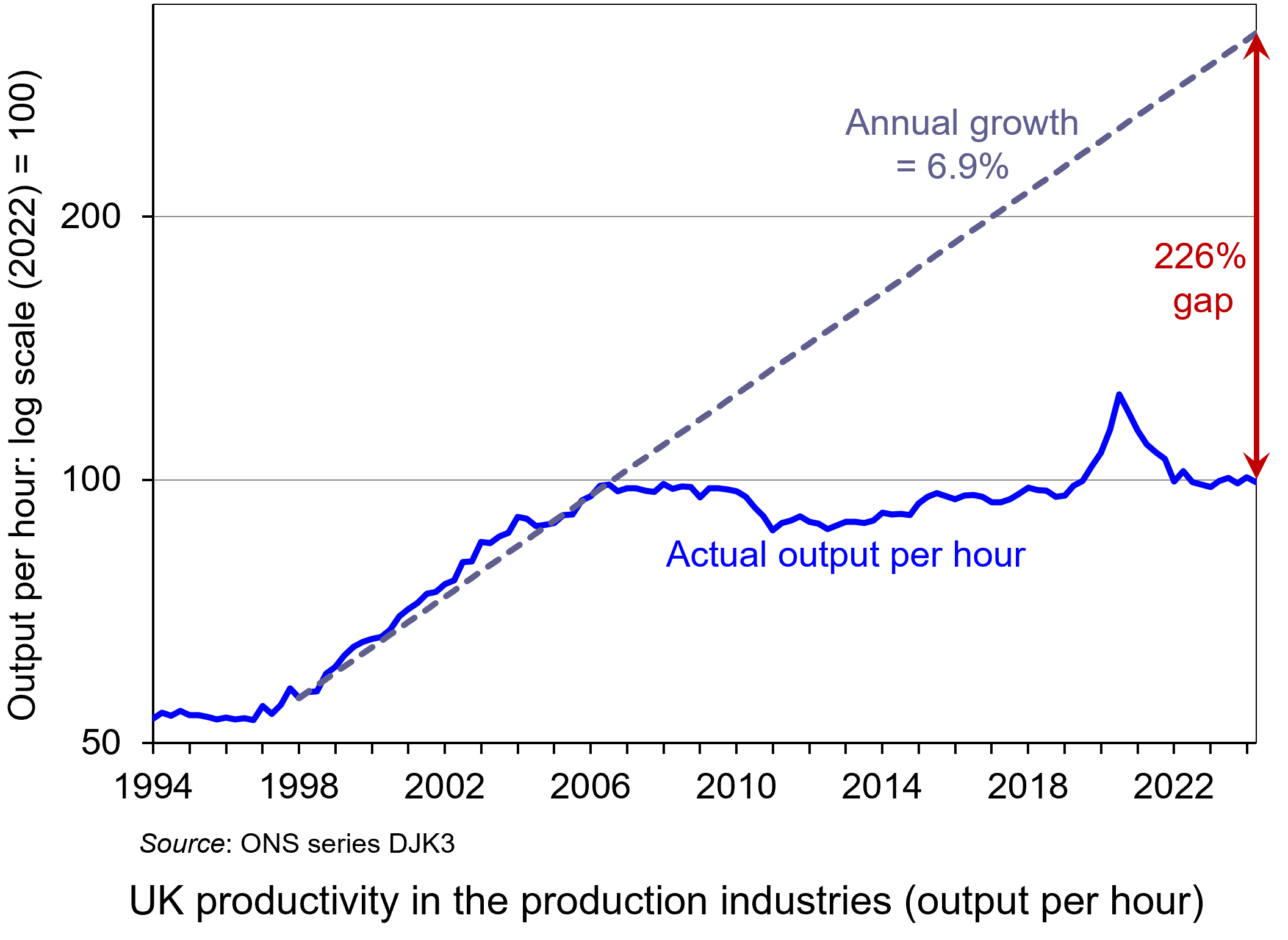 Since the financial crisis of 2007–8, the growth in UK productivity has been sluggish. This is illustrated in the chart, which looks at the production industries: i.e. it excludes services, where average productivity growth tends to be slower. The chart has been updated to 2024 Q2 – the latest data available. (Click here for a PowerPoint of the chart.)
Prior to the crisis, from 1998 to 2006, UK productivity in the production industries grew at an annual rate of 6.9%. From 2007 to the start of the pandemic in 2020, the average annual productivity growth rate in these industries was a mere 0.2%.
It grew rapidly for a short time at the start of the pandemic, but this was because many businesses temporarily shut down or went to part-time working, and many of these temporary job cuts were low-wage/low productivity jobs. If you take services, the effect was even stronger as sectors such as hospitality, leisure and retail were particularly affected and labour productivity in these sectors tends to be low. As industries opened up and took on more workers, so average productivity rapidly fell back. Since then productivity has flatlined.
If you project the average productivity growth rate from 1998 to 2007 of 6.9% forwards (see grey dashed line), then by 2024 Q3, output per hour in the production industries would have been 3.26 times higher than it actually was: a gap of 226%. This is a huge productivity gap.
 Productivity in the UK is lower than in many other competitor countries. According to the ONS, output per hour in the UK in 2021 was $59.14 in the UK. This compares with an average of $64.93 for the G7 countries, $66.75 in France, £68.30 in Germany, $74.84 in the USA, $84.46 in Norway and $128.21 in Ireland. It is lower, however, in Italy ($54.59), Canada ($53.97) and Japan ($47.28).
As we saw in the blog, The UK’s poor productivity record, low UK productivity is caused by a number of factors, not least the lack of investment in physical capital, both by private companies and in public infrastructure, and the lack of investment in training. Other factors include short-termist attitudes of both politicians and management and generally poor management practices. But one cause is the poor motivation of many workers and the feeling of being overworked. One solution to this is the four-day week.
Latest evidence on the four-day week
Results have just been released of a pilot programme involving 61 companies and non-profit organisations in the UK and nearly 3000 workers. They took part in a six-month trial of a four-day week, with no increase in hours on the days worked and no loss in pay for employees – in other words, 100% of the pay for 80% of the time. The trial was a success, with 91% of organisations planning to continue with the four-day week and a further 4% leaning towards doing so.
 The model adopted varied across companies, depending on what was seen as most suitable for them. Some gave everyone Friday off; others let staff choose which day to have off; others let staff work 80% of the hours on a flexible basis.
There was little difference in outcomes across different types of businesses. Compared with the same period last year, revenues rose by an average of 35%; sick days fell by two-thirds and 57% fewer staff left the firms. There were significant increases in well-being, with 39% saying they were less stressed, 40% that they were sleeping better; 75% that they had reduced levels of burnout and 54% that it was easier to achieve a good work–life balance. There were also positive environmental outcomes, with average commuting time falling by half an hour per week.
There is growing pressure around the world for employers to move to a four-day week and this pilot provides evidence that it significantly increases productivity and well-being.
Additional articles
Original set of articles
- Results from world’s largest 4 day week trial bring good news for the future of work
4 Day Week Global, Charlotte Lockhart (21/2/23)
- Four-day week: ‘major breakthrough’ as most UK firms in trial extend changes
The Guardian, Heather Stewart (21/2/23)
- Senedd committee backs four-day working week trial in Wales
The Guardian, Steven Morris (24/1/23)
- ‘Major breakthrough’: Most firms say they’ll stick with a four-day working week after successful trial
Sky News, Alice Porter (21/2/23)
- Major four-day week trial shows most companies see massive staff mental health benefits and profit increase
Independent, Anna Wise (21/2/23)
- Four-day week: Which countries have embraced it and how’s it going so far?
euronews, Josephine Joly and Luke Hurst (23/2/23)
- Firms stick to four-day week after trial ends
BBC News, Simon Read, Lucy Hooker & Emma Simpson (21/2/23)
- The climate benefits of a four-day workweek
BBC Future Planet, Giada Ferraglioni and Sergio Colombo (21/2/23)
- Four-day working week: why UK businesses and workers will continue with new work pattern, plus pros and cons
National World, Rochelle Barrand (22/2/23)
- Most companies in UK four-day week trial to continue with flexible working
Financial Times, Daniel Thomas and Emma Jacobs (21/2/23)
- The pros and cons of a four-day working week
Financial Times, Editorial (13/2/23)
- Explaining the UK’s productivity slowdown: Views of leading economists
VoxEU, Ethan Ilzetzki (11/3/20)
- Why the promised fourth industrial revolution hasn’t happened yet
The Conversation, Richard Markoff and Ralf Seifert (27/2/23)
Questions
- What are the possible advantages of moving to a four-day week?
- What are the possible disadvantages of moving to a four-day week?
- What types of companies or organisations are (a) most likely, (b) least likely to gain from a four-day week?
- Why has the UK’s productivity growth been lower than that of many of its major competitors?
- Why, if you use a log scale on the vertical axis, is a constant rate of growth shown as a straight line? What would a constant rate of growth line look like if you used a normal arithmetical scale for the vertical axis?
- Find out what is meant by the ‘fourth industrial revolution’. Does this hold out the hope of significant productivity improvements in the near future? (See, for example, last link above.)
 On 25 October 2024, Moody’s, one of the major credit ratings agencies, announced that it was downgrading France’s economic outlook to negative. This was its first downgrading of France since 2012. It followed a similar revision by Fitch’s, another ratings agency, on 11 October.
While Fitch’s announcement did not have a significant impact on the yields of French government bonds, expectations around Moody’s did. In the week preceding the announcement, the net increases in the yield on generic 10-year government debt was approximately 9 basis points (0.09 percentage points). On the day itself, the yield rose by approximately 5.6 basis points (0.056 percentage points).
The yield rose further throughout the rest of October, finishing nearly 0.25 percentage points above its level at the start of the month. However, as Figure 1 illustrates, these increases are part of a longer-term trend of rising yields for French government debt (click here for a PowerPoint).
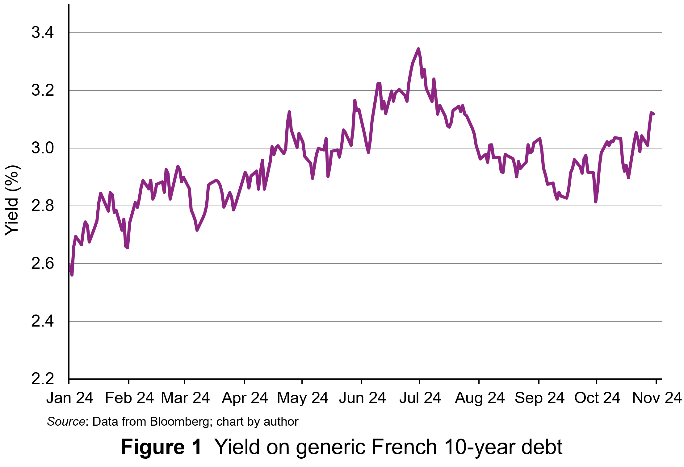 The yield on 10-year French government debt began 2024 at 2.56% and had an upward trend for the first half of the year. The yield peaked at 3.34% on 1 July. It then fell back below 3% for a while. The negative economic outlook then pushed yields back above 3% and they finished October at 3.12%, half a percentage point above the level at the start of the year. This represents a significant increase in borrowing costs for the French government.
In this blog, we will explain why the changes in France’s economic outlook translate into increases in yields for French government bonds. We will also analyse why yields have increased and examine the prospects for the markets in French government bonds.
Pricing signals of bond yields
A bond is a tradable debt instrument issued by governments to finance budget deficits – the difference between tax receipts and spending. Like any financial instruments, investment in bonds involves a commitment of funds today in anticipation of interest payments through time as compensation, with a repayment of its redemption value on the date the bond matures.
Since the cash flows associated with holding a bond occur at different points in time, discounted cash flow analysis is used to determine its value. This gives the present value of the cash flows discounted at the appropriate expected rate of return. In equilibrium this will be equal to the bond’s market price, as the following equation shows.

Where:
P = the equilibrium price of the bond
C = cash coupon payments
M = redemption value at maturity
r = yield (expected rate of return in equilibrium.
Interest payments tend to be fixed at the time a bond is issued and reflect investors’ expected rate of return, expressed as the yield in bond markets. This is determined by prevailing interest rates and perceived risk. Over time, changes in interest rates and perceptions of risk will change the expected rate of return (yield), which will, in turn, change the present value of the cash flows, and hence fundamental value.
Prices move in response to changes in fundamental value and since this happens frequently, this means that prices change a lot. For bonds, as the coupon payments (C each year and the redemption price () are fixed, the only factor that can change is the expected rate of return (yield). This is reflected in the observed yield at each price.
 If the expected rate of return rises, this increases the discount rate applied to future cash flows and reduces their present value. At the current price, the fixed coupon is not sufficient to compensate investors. So, investors sell the bonds and price falls until it reaches a point where the yield offered is equal to that required. The reverse happens if the expected rate of return falls.
The significant risk associated with bonds is credit default risk – the risk that the debt will not be repaid. The potential for credit default is a significant influence of the compensation investors require for holding debt instruments like bonds (ceteris paribus). An increase in expected credit default risk will increase the expected return (compensation). This will be reflected in a lower price and higher yield.
Normally, with the bonds issued by high-income countries, such as those in Europe and North America, the risk of default is extremely low. However, if a country’s annual deficits or accumulated debt increase to what markets consider to be unsustainable levels, the perceived risk of default may rise. Countries’ levels of risk are rated by international ratings agencies, such as Moody’s and Fitch. Investors pay a lot of attention to the information provided by such agencies.
Moody’s downgrade in its economic outlook for France from ‘stable’ to ‘negative’ indicated weak economic performance and higher credit default risk. This revision rippled through bond markets as investors adjusted their views of the country’s economic risk. The rise in yields observed is a signal that bond investors perceive higher credit default risk associated with French government debt and are demanding a higher rates of return as compensation.
Why has France’s credit default risk premium risen now?
As we have seen, credit default risk is not normally considered a significant issue for sovereign borrowers like France. Some of the issue around perceived credit default risk for the French government relate to the size of the French government’s deficit and the projections for it. Following a spike in borrowing associated with the COVID-19 pandemic in 2020, the annual government budget deficit and the overall level of debt as percentages of GDP have remained high. The annual deficit is projected to be 6% for 2024 and still 5% for 2025. The ratio of outstanding French government debt to Gross Domestic Product (GDP) ballooned to 123% in 2020 and is still expected to be 115% by the end of 2025. France has been put on notice to reduce its debt towards the Eurozone limit of 60% of GDP.
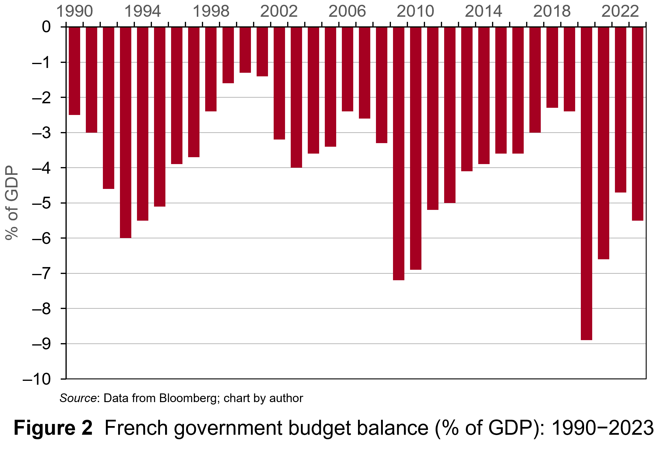 Governments in France last achieved a balanced budget in 1974. They have run deficits ever since. Figure 2 illustrates the French government budget deficits from 1990 to 2023 (click here for a PowerPoint). The figure shows that France experienced deficits in the past similar to today’s. These, however, did not tend to worry bond markets too much.
So why are investors currently worried? This stems from France’s debt mountain and from concerns that the government will not be able to deal with it. Investors are concerned that both weak growth and increasingly volatile politics will thwart efforts to reduce debt levels.
Let’s take growth. Even by contemporary European standards, France’s growth prospects are anaemic. GDP is expected to grow by just 1.1% for 2024 and 1% for 2025. Both consumer and business confidence are low. None of this suggests a growth spurt soon which will boost the tax revenues of the French government sufficiently to address the deficit.
 Further, political instability has grown due to the inconclusive parliamentary elections which Emmanuel Macron surprisingly called in July. No single political grouping has a majority and the President has appointed a Centrist Prime Minister, Michel Barnier (the former EU Brexit negotiator). His government is trying to pass a budget through the Assemblée Nationale involving a mixture of spending cuts and tax hikes which amount to savings of €60 billion ($66 billion). This is equivalent to 2% of GDP.
The parliamentary path of the budget bill is set to be torturous with both the left and right wing blocs in the Assemblée opposing most of the provisions. Debate in the Assemblée Nationale and Senate are expected to drag on into December, with the real prospect that the government may have to use presidential decree to pass the budget. Commentators argue that this will fuel further political chaos.
France looks more like Southern Europe
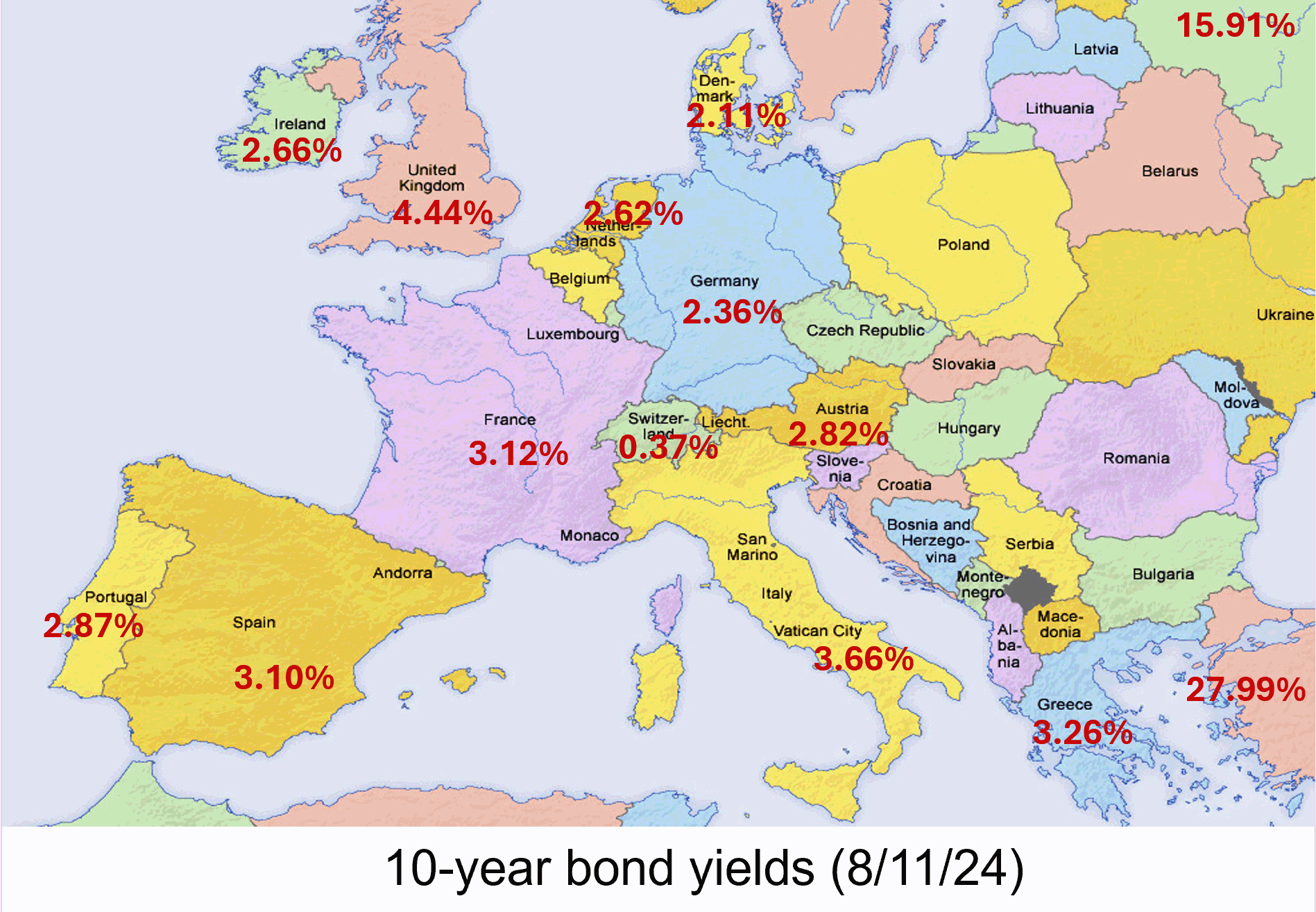 In the past, bond investors were more tolerant of France’s budget deficits. French government bonds were attractive options for investors wanting to hold euro-denominated bonds while avoiding riskier Southern European countries such as Greece, Italy, Portugal and Spain. Since France has run persistent government deficits for a long time, it offered bond investors a more liquid market than more fiscally-parsimonious Northern European neighbours, such as Germany and the Netherlands. Consequently, France’s debt instruments offered a slight risk premium on the yields for those countries.
However, that has changed. France’s credit default risk premium is rising to levels comparable to its Southern neighbours. On 26 September 2024, the yield on generic French government 10-year debt rose above its Spanish equivalent for the first time since 2008.
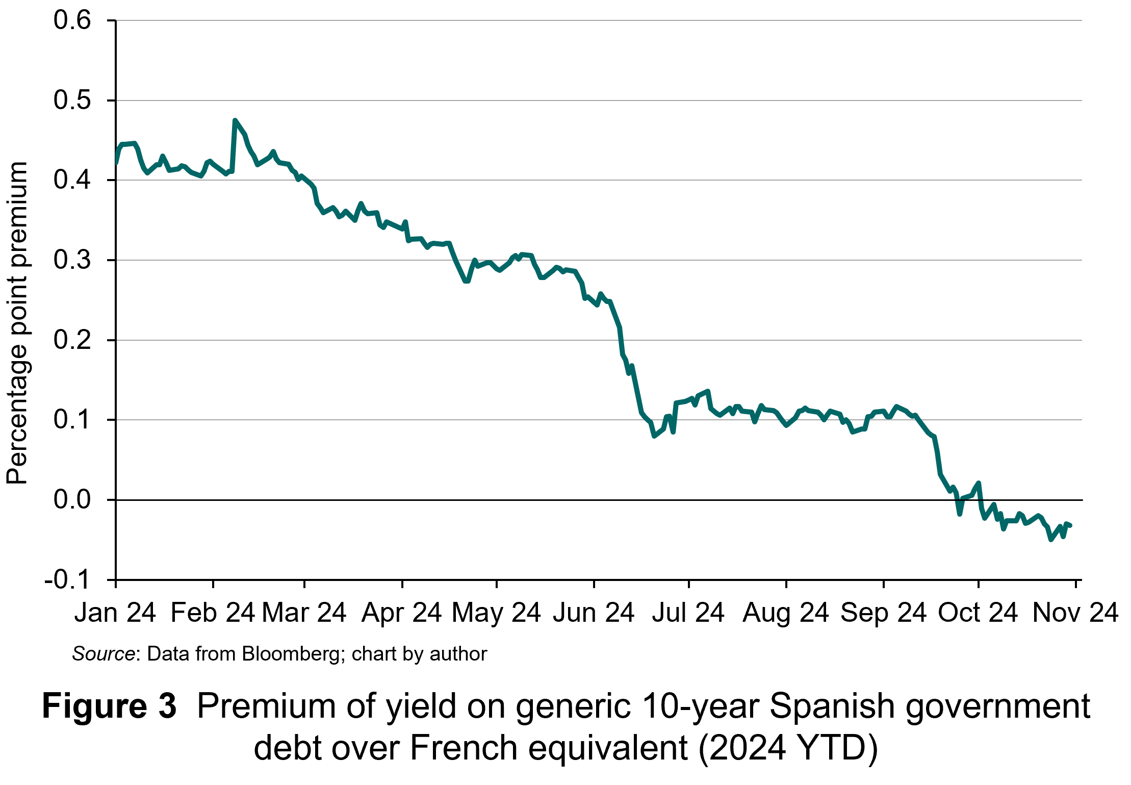 As Figure 3 illustrates, this was the culmination of a trend evident throughout 2024, with the difference in yields between the two declining steadily (click here for a PowerPoint). At the start of the year, the yield on Spanish debt offered a 40 basis points premium over the French equivalent. By October, the yield on Spanish debt was consistently below that of French debt. All of this is due to bond investors’ rising expectations about France’s credit default risk. Now, France’s borrowing costs are not only above Spain, but also closer to those of Greece and Italy than of Germany.
Strikingly, Spain’s budget deficit was 3.5% in 2023 and is expected to narrow to 2.6% by 2025. The percentage of total debt to GDP is 104% and falling. Moreover, following Spain’s inconclusive election in 2023, the caretaker government put forward budgetary plans involving fiscal tightening without the need for legislation. This avoided the political wrangling France is facing.
For France, these developments raise the prospect of yields rising further as bond investors now see alternatives to French government debt in the form of Spain’s. This country have already undertaken the painful fiscal adjustments that France seems incapable of completing.
Articles
Data
Questions
- What is credit default risk?
- Explain why higher credit default risk is associated with higher yields on France’s government debt.
- Why would low economic growth worsen the government’s budget deficit?
- Why would political instability increase credit default risk?
- What has happened to investors’ perceptions of the risk associated with French government debt relative to Spain’s?
- How has this manifested itself in the relative yields of the two countries’ government debt?
 At the fourth anniversary of Russia’s invasion of Ukraine, we look at the effect of the war on the Russian economy. Two years ago, in the blog The Russian economy after two years of war, we argued that the Russian economy had seemingly weathered the war successfully.
 But two years further on, the Russian economy is looking a lot weaker and on the verge of recession. GDP growth fell to 0.6 per cent in 2025 and is forecast to be no more than 1 per cent for the next two years. (Click here for a PowerPoint of the chart.) And despite growth still being positive (just), this is largely because of the growth in military expenditure. Retail and wholesale trade fell by 1.1% in 2025, reflecting supply chain problems and high inflation dampening consumer demand.
 Official CPI inflation averaged 8.7 per cent in 2025, although the prices of food and other consumer essentials rose by more, especially in recent months. At the beginning of 2026, supermarket prices rose by 2.3% in just one month, made worse by a rise in VAT from 20% to 22%. The central bank has responded to the high inflation with high interest rates, which averaged 19.2% in 2025, giving a real rate of 10.5%. With such a high real rate, the response of households has been to save. This has masked the constraints on production, or imports, of consumer goods. Savings have also been boosted by large payments to soldiers and bereaved families, with the money saved by the recipients being used in part to fund future such payments. So far there has been trust in the banking system, but if that trust waned and people starting making large withdrawals of savings, it could be seriously destabilising.
 The balance of payments and government finances are turning less favourable. The balance of trade surplus has declined from US$173bn in 2021 to US$67bn in 2025. This could decline further, or even become a deficit, if oil prices continue to be weak, if Western sanctions are tightened (such as stopping the flow of Russian oil exports in the ‘shadow’ fleet of tankers) or if major importing countries stop buying Russian oil. Indian refiners have announced that they are not taking Russian crude in March/April as India seeks to finalise a trade deal with the USA.
  What to Expect From the Russian Economy in 2026
 “Several think tanks warning of a recession in Russia”: Russian paper
 ‘This party is almost over’, expert says as Russia slashes 2025 forecast
 The approach towards mergers remains the most controversial area of competition policy. Some argue that policy makers in both the UK and EU have been too easily persuaded by the arguments put forward by firms and so have allowed too many mergers to proceed. Others claim that the opposite is true and that merger policy has prohibited mergers that should have been allowed to proceed. This, then, has a negative impact on investment, innovation, productivity and growth.
 In February 2025, in response to this criticism, the CMA launched its new ‘4 Ps’ approach to merger policy: Pace, Predictability, Proportionality and Process. Various changes to the investigation process have been proposed in the past 12 months using this framework.
  Proportionality. Proportionality refers to the objective of addressing any competition issues in merger cases in a way that places the minimum burden on the businesses involved. To improve proportionality, the CMA has indicated that in future cases it will be more willing to use behavioural remedies – requiring firms to take or desist from certain actions. New draft guidelines identify more situations where the use of behavioural remedies may be appropriate. However, they also show that the CMA still views structural remedies (e.g. preventing the merger or requiring firms to demerge or to sell certain assets) as more effective in many situations. Another important measure to improve proportionality is the introduction of a new ‘wait and see’ approach to global mergers. The CMA will now wait to see if the actions taken by other competition authorities in global cases address any concerns in the UK market before deciding whether to launch a review.
  The productivity gap between the UK and its main competitors is significant. In 2024, compared to the UK, output per hour worked was 10.0% higher in France, 19.8% higher in Germany and 41.1% higher in the USA. These percentages are in purchasing-power parity terms: in other words, they reflect the purchasing power of the respective currencies – the pound, the euro and the US dollar.
 The productivity gap is not a new phenomenon. It has been substantial and growing over the past 20 years. (The exception was in 2020 during lockdowns when many of the least productive sectors, such as hospitality, were forced to close temporarily.)

 Encouraging investment. Over the years, UK governments have increased investment allowances, enabling firms to offset the cost of investment against pre-tax profit, thereby reducing their tax liability. For example, in the UK, companies can offset a multiple of research and development costs against corporation tax. The rate of relief for small and medium-sized enterprises (SMEs) allows companies that work in science and technology to deduct an extra 86% of their qualifying expenditure from their trading profit in addition to the normal 100% deduction: i.e. a total of 186% deduction. Meanwhile, since April 2016, larger companies have been able to claim a R&D expenditure credit, initially worth 11 per cent of R&D expenditures, then 12 per cent from 2018 and 13 per cent from 2020. This was then raised to 20 per cent from 2023.
 They also discuss the role that AI plays, or could play, in doing otherwise time-consuming tasks, such as recording and paying invoices and record keeping in offices; writing grants or producing policy documents; analysing X-ray results in hospitals and performing preliminary diagnoses when patients present with various symptoms; recording conversations/consultations and then sorting, summarising and transcribing them; building AI capabilities into machines or robots to enable them to respond to different specifications or circumstances; software development where AI writes the code. Often, there is a shortage of time for workers to do more creative things. AI can help release more time by doing a lot of the mundane tasks or allowing people to do them much quicker.
 In a blog from March 2023 (reproduced below), we saw how there has been growing pressure around the world for employers to move to a four-day week. Increasing numbers of companies have adopted the model of 80% of the hours for 100% of the pay.
 Since the financial crisis of 2007–8, the growth in UK productivity has been sluggish. This is illustrated in the chart, which looks at the production industries: i.e. it excludes services, where average productivity growth tends to be slower. The chart has been updated to 2024 Q2 – the latest data available. (Click
  Productivity in the UK is lower than in many other competitor countries.
  On 25 October 2024, Moody’s, one of the major credit ratings agencies, announced that it was downgrading France’s economic outlook to negative. This was its first downgrading of France since 2012. It followed a similar revision by Fitch’s, another ratings agency, on 11 October.
 The yield on 10-year French government debt began 2024 at 2.56% and had an upward trend for the first half of the year. The yield peaked at 3.34% on 1 July. It then fell back below 3% for a while. The negative economic outlook then pushed yields back above 3% and they finished October at 3.12%, half a percentage point above the level at the start of the year. This represents a significant increase in borrowing costs for the French government.
 If the expected rate of return rises, this increases the discount rate applied to future cash flows and reduces their present value. At the current price, the fixed coupon is not sufficient to compensate investors. So, investors sell the bonds and price falls until it reaches a point where the yield offered is equal to that required. The reverse happens if the expected rate of return falls.
  Governments in France last achieved a balanced budget in 1974. They have run deficits ever since. Figure 2 illustrates the French government budget deficits from 1990 to 2023 (click
  Further, political instability has grown due to the inconclusive parliamentary elections which Emmanuel Macron surprisingly called in July. No single political grouping has a majority and the President has appointed a Centrist Prime Minister, Michel Barnier (the former EU Brexit negotiator). His government is trying to pass a budget through the Assemblée Nationale involving a mixture of spending cuts and tax hikes which amount to savings of €60 billion ($66 billion). This is equivalent to 2% of GDP.
 In the past, bond investors were more tolerant of France’s budget deficits. French government bonds were attractive options for investors wanting to hold euro-denominated bonds while avoiding riskier Southern European countries such as Greece, Italy, Portugal and Spain. Since France has run persistent government deficits for a long time, it offered bond investors a more liquid market than more fiscally-parsimonious Northern European neighbours, such as Germany and the Netherlands. Consequently, France’s debt instruments offered a slight risk premium on the yields for those countries.
  As Figure 3 illustrates, this was the culmination of a trend evident throughout 2024, with the difference in yields between the two declining steadily (click