 The past decade or so has seen large-scale economic turbulence. As we saw in the blog Fiscal impulses, governments have responded with large fiscal interventions. The COVID-19 pandemic, for example, led to a positive fiscal impulse in the UK in 2020, as measured by the change in the structural primary balance, of over 12 per cent of national income.
The scale of these interventions has led to a significant increase in the public-sector debt-to-GDP ratio in many countries. The recent interest rates hikes arising from central banks responding to inflationary pressures have put additional pressure on the financial well-being of governments, not least on the financing of their debt. Here we discuss these pressures in the context of the ‘r – g’ rule of sustainable public debt.
Public-sector debt and borrowing
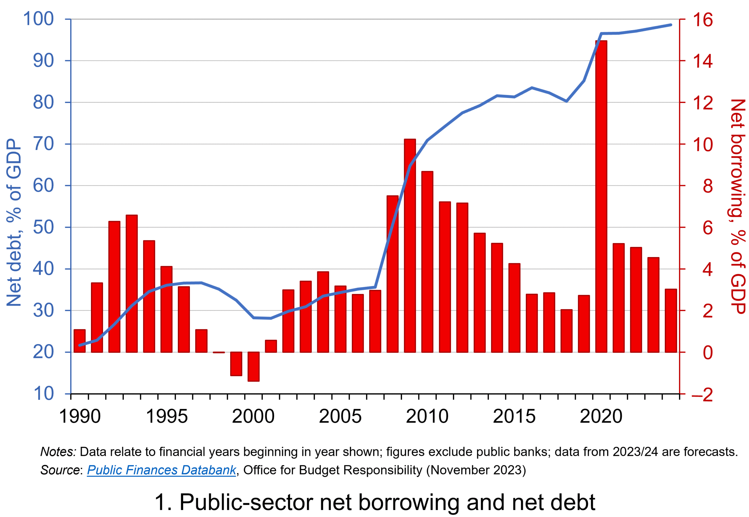 Chart 1 shows the path of UK public-sector net debt and net borrowing, as percentages of GDP, since 1990. Debt is a stock concept and is the result of accumulated flows of past borrowing. Net debt is simply gross debt less liquid financial assets, which mainly consist of foreign exchange reserves and cash deposits. Net borrowing is the headline measure of the sector’s deficit and is based on when expenditures and receipts (largely taxation) are recorded rather than when cash is actually paid or received. (Click here for a PowerPoint of Chart 1)
Chart 1 shows the impact of the fiscal interventions associated with the global financial crisis and the COVID-19 pandemic, when net borrowing rose to 10 per cent and 15 per cent of GDP respectively. The former contributed to the debt-to-GDP ratio rising from 35.6 per cent in 2007/8 to 81.6 per cent in 2014/15, while the pandemic and subsequent cost-of-living interventions contributed to the ratio rising from 85.2 per cent in 2019/20 to around 98 per cent in 2023/24.
Sustainability of the public finances
 The ratcheting up of debt levels affects debt servicing costs and hence the budgetary position of government. Yet the recent increases in interest rates also raise the costs faced by governments in financing future deficits or refinancing existing debts that are due to mature. In addition, a continuation of the low economic growth that has beset the UK economy since the global financial crisis also has implications for the burden imposed on the public sector by its debts, and hence the sustainability of the public finances. After all, low growth has implications for spending commitments, and, of course, the flow of receipts.
The analysis therefore implies that the sustainability of public-sector debt is dependent on at least three factors: existing debt levels, the implied average interest rate facing the public sector on its debts, and the rate of economic growth. These three factors turn out to underpin a well-known rule relating to the fiscal arithmetic of public-sector debt. The rule is sometimes known as the ‘r – g’ rule (i.e. the interest rate minus the growth rate).
Underpinning the fiscal arithmetic that determines the path of public-sector debt is the concept of the ‘primary balance’. This is the difference between the sector’s receipts and its expenditures less its debt interest payments. A primary surplus (a positive primary balance) means that receipts exceed expenditures less debt interest payments, whereas a primary deficit (a negative primary balance) means that receipts fall short. The fiscal arithmetic necessary to prevent the debt-to-GDP ratio rising produces the following stable debt equation or ‘r – g’ rule:
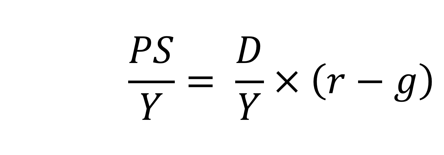
On the left-hand side of the stable debt equation is the required primary surplus (PS) to GDP (Y) ratio. Moving to the right-hand side, the first term is the existing debt-to-GDP ratio (D/Y). The second term ‘r – g’, is the differential between the average implied interest rate the government pays on its debt and the growth rate of the economy. These terms can be expressed in either nominal or real terms as this does not affect the differential.
To illustrate the rule consider a country whose existing debt-to-GDP ratio is 1 (i.e. 100 per cent) and the ‘r – g’ differential is 0.02 (2 percentage points). In this scenario they would need to run a primary surplus to GDP ratio of 0.02 (i.e. 2 percent of GDP).
The ‘r – g‘ differential
The ‘r – g’ differential reflects macroeconomic and financial conditions. The fiscal arithmetic shows that these are important for the dynamics of public-sector debt. The fiscal arithmetic is straightforward when r = g as any primary deficit will cause the debt-to-GDP ratio to rise, while a primary surplus will cause the ratio to fall. The larger is g relative to r the more favourable are the conditions for the path of debt. Importantly, if the differential is negative (r < g), it is possible for the public sector to run a primary deficit, up to the amount that the stable debt equation permits.
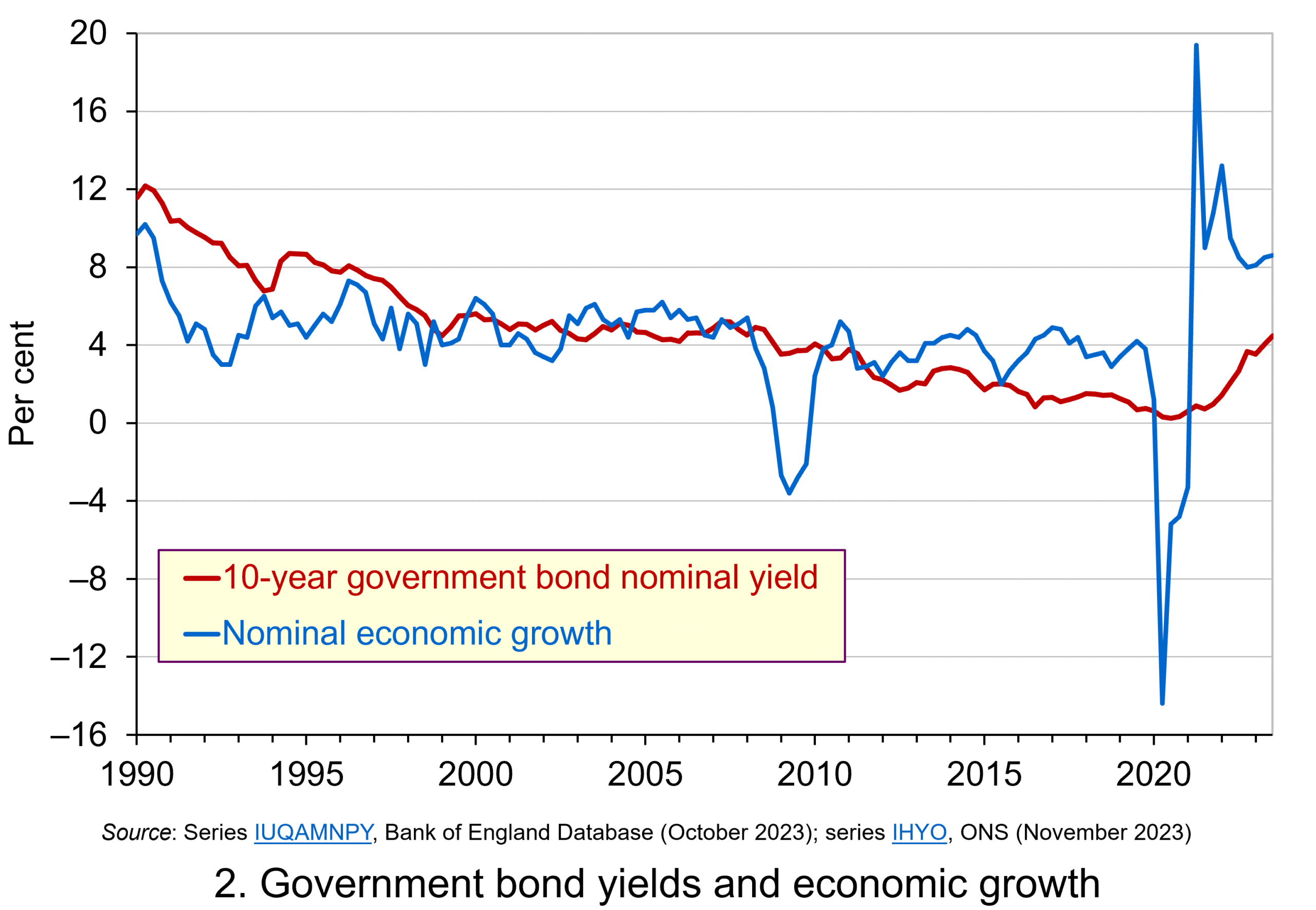 Consider Charts 2 and 3 to understand how the ‘r – g’ differential has affected debt sustainability in the UK since 1990. Chart 2 plots the implied yield on 10-year government bonds, alongside the annual rate of nominal growth (click here for a PowerPoint). As John explains in his blog The bond roller coaster, the yield is calculated as the coupon rate that would have to be paid for the market price of a bond to equal its face value. Over the period, the average annual nominal growth rate was 4.5 per cent, while the implied interest rate was almost identical at 4.6 per cent. The average annual rate of CPI inflation over this period was 2.8 per cent.
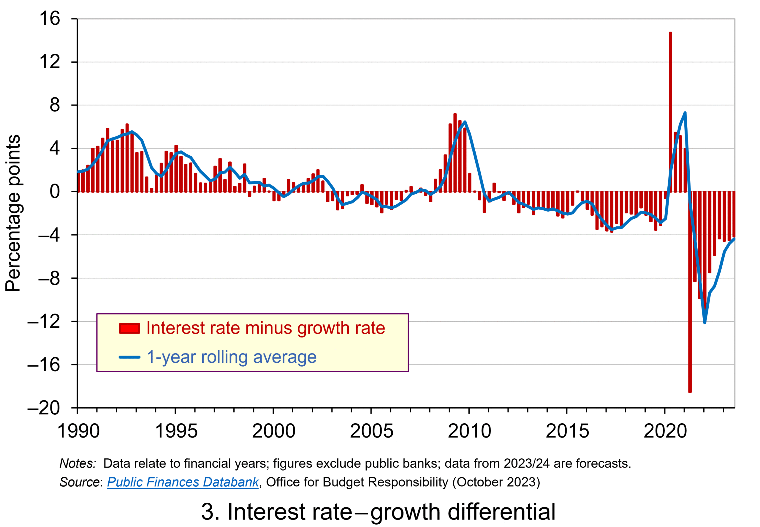 Chart 3 plots the ‘r – g’ differential which is simply the difference between the two series in Chart 2, along with a 12-month rolling average of the differential to help show better the direction of the differential by smoothing out some of the short-term volatility (click here for a PowerPoint). The differential across the period is a mere 0.1 percentage points implying that macroeconomic and financial conditions have typically been neutral in supporting debt sustainability. However, this does mask some significant changes across the period.
We observe a general downward trend in the ‘r – g’ differential from 1990 up to the time of the global financial crisis. Indeed between 2003 and 2007 we observe a favourable negative differential which helps to support the sustainability of public debt and therefore the well-being of the public finances. This downward trend of the ‘r – g’ differential was interrupted by the financial crisis, driven by a significant contraction in economic activity. This led to a positive spike in the differential of over 7 percentage points.
 Yet the negative differential resumed in 2010 and continued up to the pandemic. Again, this is indicative of the macroeconomic and financial environments being supportive of the public finances. It was, however, largely driven by low interest rates rather than by economic growth.
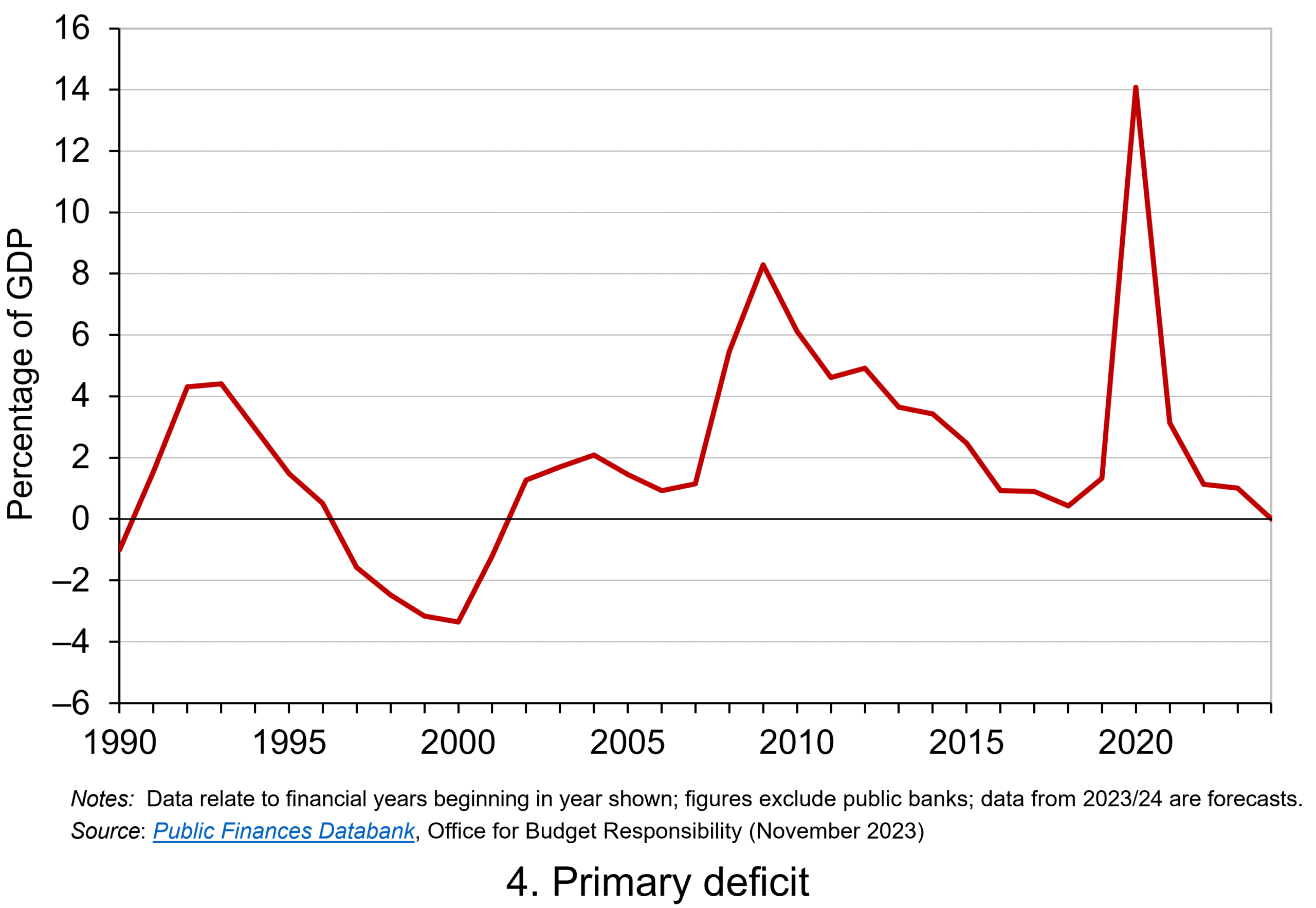
Consequently, the negative ‘r – g’ differential meant that the public sector could continue to run primary deficits during the 2010s, despite the now much higher debt-to-GDP ratio. Yet, weak growth was placing limits on this. Chart 4 indeed shows that primary deficits fell across the decade (click here for a PowerPoint).
The pandemic and beyond
 The pandemic saw the ‘r – g’ differential again turn markedly positive, averaging 7 percentage points in the four quarters from Q2 of 2020. While the differential again turned negative, the debt-to-GDP ratio had also increased substantially because of large-scale fiscal interventions. This made the negative differential even more important for the sustainability of the public finances. The question is how long the negative differential can last.
Looking forward, the fiscal arithmetic is indeed uncertain and worryingly is likely to be less favourable. Interest rates have risen and, although inflationary pressures may be easing somewhat, interest rates are likely to remain much higher than during the past decade. Geopolitical tensions and global fragmentation pose future inflationary concerns and a further drag on growth.
As well as the short-term concerns over growth, there remain long-standing issues of low productivity which must be tackled if the growth of the UK economy’s potential output is to be raised. These concerns all point to the important ‘r – g’ differential become increasingly less negative, if not positive. If so the fiscal arithmetic could mean increasingly hard maths for policymakers.
Articles
- The budget deficit: a short guide
House of Commons Library (8/6/23)
- If markets are right about long real rates, public debt ratios will increase for some time. We must make sure that they do not explode.
Peterson Institute for International Economics, Olivier Blanchard (6/11/23)
- The UK government’s debt nightmare
ITV News, Robert Peston (13/7/23)
- National debt could hit 300% of GDP by 2070s, independent watchdog the OBR warns
Sky News, James Sillars (13/7/23)
- How much money is the UK government borrowing, and does it matter?
BBC News (20/10/23)
- Cost of national debt hits 20-year high
BBC News, Vishala Sri-Pathma & Faisal Islam (4/10/23)
- Bond markets could see ‘mini boom-bust cycles’ as global government debt to soar by $5 trillion a yea
Markets Insider, Filip De Mott (16/11/23)
- The counterintuitive truth about deficits for bond investors
Financial Times, Matt King (17/11/23)
- UK government borrowing almost £20bn lower than expected
The Guardian, Richard Partington (20/10/23)
- Controlling debt is just a means — it is not a government’s end
Financial Times, Martin Wolf (13/11/23)
Data
Questions
- What is meant by each of the following terms: (a) net borrowing; (b) primary deficit; (c) net debt?
- Explain how the following affect the path of the public-sector debt-to-GDP ratio: (a) interest rates; (b) economic growth; (c) the existing debt-to-GDP ratio.
- Which factors during the 2010s were affecting the fiscal arithmetic of public debt positively, and which negatively?
- Discuss the prospects for the fiscal arithmetic of public debt in the coming years.
- Assume that a country has an existing public-sector debt-to-GDP ratio of 60 percent.
(a) Using the ‘rule of thumb’ for public debt dynamics, calculate the approximate primary balance it would need to run in the coming year if the expected average real interest rate on the debt were 3 per cent and real economic growth were 2 per cent?
(b) Repeat (a) but now assume that real economic growth is expected to be 4 per cent.
(c) Repeat (a) but now assume that the existing public-sector debt-to-GDP ratio is 120 per cent.
(d) Using your results from (a) to (c) discuss the factors that affect the fiscal arithmetic of the growth of public-sector debt.
 To make a sensible comparison of one year’s national income generated from the production of goods and services with another we need to take inflation into account. Changes in inflation-adjusted GDP represent changes in the volume of production of a country’s goods and services: in other words, the real value of goods and services. We revisit the blog written back in April 2019, prior the pandemic, to show how changes in real GDP evidence what we may refer to as the twin characteristics of economic growth: positive long-term growth but with fluctuating short-term rates of growth.
Real and nominal GDP
The nominal or current-price estimate for UK Gross Domestic Product in 2020 is £2.156 trillion. It is the value of output produced within the country in 2020. This was a fall of 4.4 per cent on the £2.255 trillion recorded in 2019. These values make no adjustment for inflation and therefore reflect the prices of output that were prevailing at the time.
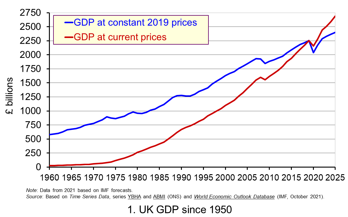 Chart 1 shows current-price estimates of GDP from 1950 when the value of GDP was estimated at £12.7 billion. The increase to £2.156 trillion in 2020 amounts to a proportionate increase of almost 170 times, a figure that rises to 211 times if we compare the 1950 value with the latest IMF estimate for 2025 of £2.689 trillion. However, if we want to make a more meaningful comparison of the country’s national income by looking at the longer-term increase in the volume of production, we need to adjust for inflation. (Click here to download a PowerPoint copy of the chart.)
Long-term growth in real GDP
If we measure GDP at constant prices, we eliminate the effect of inflation. To construct a constant-price series for GDP a process known as chain-linking is used. This involves taking consecutive pairs of years, e.g. 2020 and 2021, and estimating what GDP would be in the most recent year (in this case, 2021) if the previous year’s prices (i.e. 2020) had continued to prevail. By calculating the percentage change from the previous year’s GDP value we have an estimate of the volume change. If this is repeated for other pairs of years, we have a series of percentage changes that capture the volume changes from year-to-year. Finally, a reference year is chosen and the percentage changes are applied backwards and forwards from the nominal GDP value for the reference year – the volume changes forwards and backwards from this point.
In effect, a real GDP series creates a quantity measure in monetary terms. Chart 1 shows GDP at constant 2019 prices (real GDP) alongside GDP at current prices (nominal GDP). Consider first the real GDP numbers for 1950 and 2020. GDP in 1950 at 2019 prices was £410.1 billion. This is higher than the current-price value because prices in 2019 (the reference year) were higher than those in 1950. Meanwhile, GDP in 2020 when measured at 2019 prices was £2.037 trillion. This constant-price value is smaller than the corresponding current-price value because prices in 2019 where lower than those in 2020.
Between 1950 and 2020 real GDP increased 5.0 times. If we extend the period to 2025, again using the latest IMF estimates, the increase is 5.9 times. Because we have removed the effect of inflation, the real growth figure is much lower than the nominal growth figure. Crucially, what we are left with is an indicator of the long-term growth in the volume of the economy’s output and hence an increase in national income that is backed up by an increase in production. Whereas nominal growth rates are affected both by changes in volumes and prices, real growth rates reflect only changes in volumes.
The upward trajectory observed in constant-price GDP is therefore evidence of positive longer-term growth. This is one of the twin characteristics of growth.
Short-term fluctuations in the growth of real GDP
The second characteristic is fluctuations in the rate of growth from period to period. We can see this second characteristic more clearly by plotting the percentage change in real GDP from year to year.
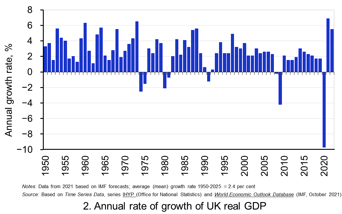 Chart 2 shows the annual rate of growth in real GDP each year since 1950. From it, we see the inherent instability that is a key characteristic of the macroeconomic environment. This instability is, of course, mirrored in the output path of real GDP in Chart 1, but the annual rates of growth show the instability more clearly. We can readily see the impact on national output of the global financial crisis and the global health emergency.
In 2009, constant-price GDP in the UK fell by 4.25 per cent. Then, in 2020, constant-price GDP and, hence, the volume of national output fell by 9.7 per cent, as compared to a 4.4 per cent fall in current-price GDP that we identified earlier. These global, ‘once-in-a-generation’ shocks are stark examples of the instability that characterises economies and which generate the ‘ups and downs’ in an economy’s output path, known more simply as ‘the business cycle’. (Click here to download a PowerPoint copy of the chart.)
Determinants of long-and short-term growth
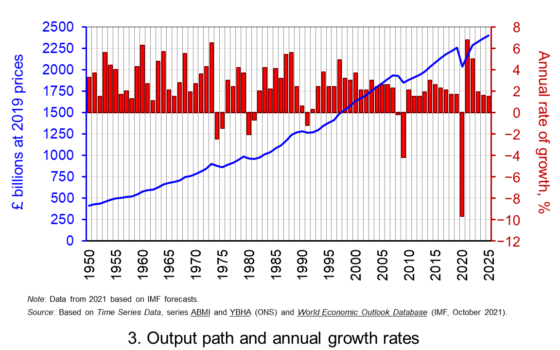 The twin characteristics of growth can be seen simultaneously by combining the output path captured by the levels of real GDP with the annual rates of growth. This is shown in Chart 3. The longer-term growth seen in the economy’s output path is generally argued to be driven by the quantity and quality of the economy’s resources, and their effectiveness when combined in production. In other words, it is the supply-side that determines the trajectory of the output path over the longer term. (Click here to download a PowerPoint copy of the chart.)
However, the fluctuations we observe in short-term growth rates tend to reflect impulses that affect the ability and or willingness of producers to supply (supply-side shocks) and purchasers to consume (demand-side shocks). These impulses are then propagated and their effects, therefore, transmitted through the economy.
Effects of the pandemic
The pandemic is unusual in that the health intervention measures employed by governments around the world resulted in simultaneous negative aggregate demand and aggregate supply shocks. Economists were particularly concerned that the magnitude of these impulses and their propagation had the potential to generate scarring effects and hence negative hysteresis effects. The concern was that these would affect the level of real GDP in the medium-to-longer term and, hence, the vertical position of the output path, as well as the longer-term rate of growth and, hence, the steepness of the output path.
The extent of these scarring effects continues to be debated. The ability of businesses and workers to adapt their practices, the extraordinary fiscal and monetary measures that were undertaken in many countries, and the roll-out of vaccines programmes, especially in advanced economies, have helped to mitigate some of these effects. For example, the latest IMF forecasts for output in the USA in 2024 are over 2 per cent higher than those made back in October 2019.
Scarring effects are, however, thought to be an ongoing issue in the UK. The IMF is now expecting output in the UK to be nearly 3 per cent lower than it originally forecast back in October 2019. Therefore, whilst UK output is set to recover, scarring effects on the UK economy will mean that the output path traced out by real GDP will remain, at least in the medium term, vertically lower than was expected before the pandemic.
Data and Reports
Articles
Questions
- What do you understand by the term ‘macroeconomic environment’? What data could be used to describe the macroeconomic environment?
- When a country experiences positive rates of inflation, which is higher: nominal economic growth or real economic growth?
- Does an increase in nominal GDP mean a country’s production has increased? Explain your answer.
- Does a decrease in nominal GDP mean a country’s production has decreased? Explain your answer.
- Why does a change in the growth of real GDP allow us to focus on what has happened to the volume of production?
- What does the concept of the ‘business cycle’ have to do with real rates of economic growth?
- When would falls in real GDP be classified as a recession?
- Distinguish between the concepts of ‘short-term growth rates’ and ‘longer-term growth’.
- What do you understand by the term hysteresis? By what means can hysteresis effects be generated?
- Discuss the proposition that the pandemic could have a positive effect on longer-term growth rates because of the ways that people and business have had to adapt.
 The coronavirus pandemic and the climate emergency have highlighted the weaknesses of free-market capitalism.
Governments around the world have intervened massively to provide economic support to people and businesses affected by the pandemic through grants and furlough schemes. They have also stressed the importance of collective responsibility in abiding by lockdowns, social distancing and receiving vaccinations.
The pandemic has also highlighted the huge inequalities around the world. The rich countries have been able to offer much more support to their people than poor countries and they have had much greater access to vaccines. Inequality has also been growing within many countries as rich people have gained from rising asset prices, while many people find themselves stuck in low-paid jobs, suffering from poor educational opportunities and low economic and social mobility.
The increased use of working from home and online shopping has accelerated the rise of big tech companies, such as Amazon and Google. Their command of the market makes it difficult for small companies to compete – and competition is vital if capitalism is to benefit societies. There have been growing calls for increased regulation of powerful companies and measures to stimulate competition. The problem has been recognised by governments, central banks and international agencies, such as the IMF and the OECD.
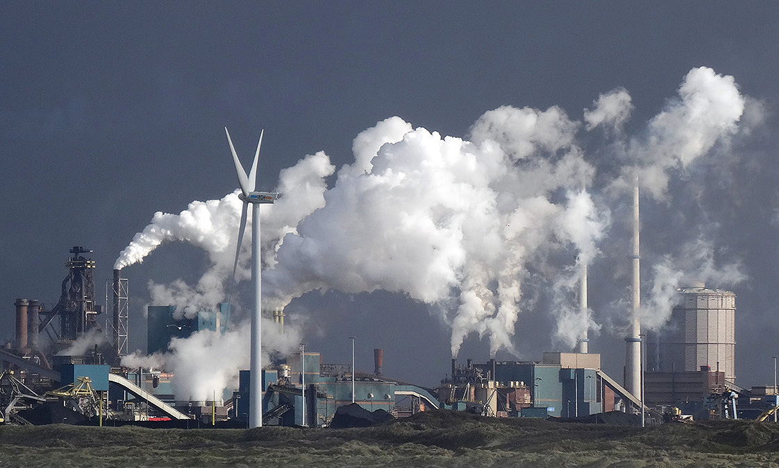 At the same time as the world has been grappling with the pandemic, global warming has contributed to extreme heat and wildfires in various parts of the world, such as western North America, the eastern Mediterranean and Siberia, and major flooding in areas such as western Europe and China. Governments again have intervened by providing support to people whose property and livelihoods have been affected. Also there is a growing urgency to tackle global warming, with some movement, albeit often limited, in implementing policies to achieve net zero carbon emissions by some specified point in the future. Expectations are rising for concerted action to be agreed at the international COP26 climate meeting in Glasgow in November this year.
An evolving capitalism
So are we seeing a new variant of capitalism, with a greater recognition of social responsibility and greater government intervention?
 Western governments seem more committed to spending on socially desirable projects, such as transport, communications and green energy infrastructure, education, science and health. They are beginning to pursue more active industrial and regional policies. They are also taking measures to tax multinationals (see the blog The G7 agrees on measures to stop corporate tax avoidance). Many governments are publicly recognising the need to tackle inequality and to ‘level up’ society. Active fiscal policy, a central plank of Keynesian economics, has now come back into fashion, with a greater willingness to fund expenditure by borrowing and, over the longer term, to use higher taxes to fund increased government expenditure.
But there is also a growing movement among capitalists themselves to move away from profits being their sole objective. A more inclusive ‘stakeholder capitalism’ is being advocated by many companies, where they take into account the interests of a range of stakeholders, from customers, to workers, to local communities, to society in general and to the environment. For example, the Council for Inclusive Capitalism, which is a joint initiative of the Vatican and several world business and public-sector leaders, seeks to make ‘the world fairer, more inclusive, and sustainable’.
If there is to be a true transformation of capitalism from the low-tax free-market capitalism of neoclassical economists and libertarian policymakers to a more interventionist mixed market capitalism, where capitalists pursue a broader set of objectives, then words have to be matched by action. Talk is easy; long-term plans are easy; taking action now is what matters.
Articles and videos
- Why the next stage of capitalism is coming
BBC Future, Matthew Wilburn King (27/5/21)
- During the pandemic, a new variant of capitalism has emerged
The Guardian, Larry Elliott (30/7/21)
- When it comes to social and environmental justice, words don’t cut it
GreenBiz, C J Clouse (28/4/21)
 Introducing the Council for Inclusive Capitalism with the Vatican
Inclusive Capitalism (7/12/20)
- The State and Direction of Inclusive Capitalism
Saïd Business School, Ford Foundation and Deloitte Social Impact practice, Richard Barker, Mary Johnstone-Louis, Colin Mayer, Pradeep Prabhala, Noah Rimland Flower, Theodore Roosevelt Malloch, Tony Siesfeld and Peter Tufano (2018)
- Rising Market Power—A Threat to the Recovery?
IMF Blog, Kristalina Georgieva, Federico J Díez, Romain Duval and Daniel Schwarz (15/3/21)
- The Pandemic Alone Can’t Transform Capitalism
Jacobin, Ramaa Vasudevan (30/7/21)
- Down to earth: How entrepreneurs can collaborate to rejuvenate capitalism
EU-Startups, Luca Sabia (4/8/21)
Questions
- How similar is the economic response of Western governments to the pandemic to their response to the financial crisis of 2007–8?
- What do you understand by ‘inclusive capitalism’? How can stakeholders hold companies to account?
- What indicators are there of market power? Why have these been on the rise?
- How can entrepreneurs contribute to ‘closing the inequality gap for a more sustainable and inclusive form of society’?
- What can be done to hold governments to account for meeting various social and environmental objectives? How successful is this likely to be?
- Can inequality be tackled without redistributing income and wealth from the rich to the poor?
 One of the major economic concerns about the COVID-19 pandemic has been the likely long-term scarring effects on economies from bankruptcies, a decline in investment, lower spending on research and development, a loss of skills, discouragement of workers, disruption to education, etc. The result would be a decline in potential output or, at best, a slower growth. These persistent effects are known as ‘hysteresis’ – an effect that persists after the original cause has disappeared.
In a speech by Dave Ramsden, the Bank of England’s Deputy Governor for Markets & Banking, he argued that, according to MPC estimates, the pandemic will have caused a loss of potential output of 1.75%. This shortfall may seem small at first sight, so does it matter? According to Ramsden:
The answer is definitely yes for two reasons. First, a 1¾% shortfall as a share of annual GDP for the UK … represents roughly £39 billion – for context, that’s about half of the education budget. And second, that 1¾% represents a permanent shortfall, or at least a very persistent one, on top of the impact of the immediate downturn. If you lose 1¾% of GDP every year for ten years, then in total you have lost 17.5% of one year’s GDP, or around £390bn in 2019 terms
However, as the IMF blog linked below argues, there may be positive supply-side effects which outweigh these scarring effects, causing a net rise in potential GDP growth. There are two possible reasons for this.
 The first is that the pandemic may have hastened the process of digitalisation and automation. Examples include ‘video conferencing and file sharing applications to drones and data-mining technologies’. According to evidence from a sample of 15 countries cited in the blog, a 10% rise in such intangible capital investment is associated with about a 4½% rise in labour productivity. ‘As COVID-19 recedes, the firms which invested in intangible assets, such as digital technologies and patents may see higher productivity as a result.’
The second is a reallocation of workers and capital to more productive sectors. Firms in some sectors, such as leisure, hospitality and retail, have relatively low labour productivity. Many parts of these industries have declined during the pandemic, especially those with high labour intensity. At the same time, there has been a rise in employment in firms where output per worker is higher. Such sectors include e-commerce and those where remote working is possible. The greater the reallocation from low labour-productivity to high labour-productivity sectors, the more will overall labour productivity rise and hence the more will potential output increase.
The size of these two effects will depend to a large extent on expectations, incentives and government policy. The blog cites four types of policy that can help investment and reallocation.
- Improved insolvency and restructuring procedures to enable capital in failed firms to be reallocated to sectors with potential for growth.
- Promoting competition to enable the exit and entry of firms into expanding sectors and to prevent powerful firms from blocking the process.
- Refocusing policy from retaining labour in existing jobs to reskilling workers for new jobs, thereby improving labour mobility from declining to expanding sectors.
- Addressing financial bottlenecks, so as to ensure adequate access to financing for viable firms.
Whether there will be a net increase or decrease in productivity from the pandemic very much depends on the extent to which firms and workers are able and willing to take advantage of new opportunities and the extent to which government supports investment in and reallocation to high-productivity sectors.
Blogs, articles and speeches
Questions
- Can actual economic growth be greater than potential economic growth (a) in the short run; (b) in the long run?
- Give some example of scarring effects from the COVID-19 pandemic.
- What effects might short-term policies to tackle the recession caused by the pandemic have on longer-term potential economic growth?
- What practical policies could governments adopt to encourage the positive supply-side effects of the pandemic? To what extent would these policies have negative short-term effects?
- Why might (endogenous) financial crises result in larger and more persistent reductions in potential output than exogenous crises, such as a pandemic or a war?
- Distinguish between interventionist and market-orientated supply-side policies to encourage the reallocation of labour and capital to higher-productivity sectors.
 Many developing countries are facing a renewed debt crisis. This is directly related to Covid-19, which is now sweeping across many poor countries in a new wave.
Between 2016 and 2020, debt service as a percentage of GDP rose from an average of 7.1% to 27.1% for South Asian countries, from 8.1% to 14.1% for Sub-Saharan African countries, from 13.1% to 42.3% for North African and Middle Eastern countries, and from 5.6% to 14.7% for East Asian and Pacific countries. These percentages are expected to climb again in 2021 by around 10% of GDP.
Incomes have fallen in developing countries with illness, lockdowns and business failures. This has been compounded by a fall in their exports as the world economy has contracted and by a 19% fall in aid in 2020. The fall in incomes has led to a decline in tax revenues and demands for increased government expenditure on healthcare and social support. Public-sector deficits have thus risen steeply.
And the problem is likely to get worse before it gets better. Vaccination roll-outs in most developing countries are slow, with only a tiny fraction of the population having received just one jab. With the economic damage already caused, growth is likely to be subdued for some time.
This has put developing countries in a ‘trilemma’, as the IMF calls it. Governments must balance the objectives of:
- meeting increased spending needs from the emergency and its aftermath;
- limiting the substantial increase in public debt;
- trying to contain rises in taxes.
Developing countries are faced with a difficult trade-off between these objectives, as addressing one objective is likely to come at the expense of the other two. For example, higher spending would require higher deficits and debt or higher taxes.
The poorest countries have little scope for increased domestic borrowing and have been forced to borrow on international markets. But such debt is costly. Although international interest rates are generally low, many developing countries have had to take on increasing levels of borrowing from private lenders at much higher rates of interest, substantially adding to the servicing costs of their debt.
Debt relief
 International agencies and groups, such as the IMF, the World Bank, the United Nations and the G20, have all advocated increased help to tackle this debt crisis. The IMF has allocated $100bn in lending through the Rapid Financing Instrument (RFI) and the Rapid Credit Facility (RCF) and nearly $500m in debt service relief grants through the Catastrophe Containment and Relief Trust (CCRT). The World Bank is increasing operations to $160bn.
The IMF is also considering an increase in special drawing rights (SDRs) from the current level of 204.2bn ($293.3bn) to 452.6bn ($650bn) – a rise of 121.6%. This would be the first such expansion since 2009. It has received the support of both the G7 and the G20. SDRs are reserves created by the IMF whose value is a weighted average of five currencies – the US dollar (41.73%), the euro (30.93%), the Chinese yuan (10.92%), the Japanese yen (8.33%) and the pound sterling (8.09%).
Normally an increase in SDRs would be allocated to countries according their IMF quotas, which largely depend on the size of their GDP and their openness. Any new allocation under this formula would therefore go mainly to developed countries, with developing economies getting only around $60bn of the extra $357bn. It has thus been proposed that developed countries give much of their allocation to developing countries. These could then be used to cancel debts. This proposal has been backed by Janet Yellen, the US Secretary of the Treasury, who said she would “strongly encourage G20 members to channel excess SDRs in support of recovery efforts in low-income countries, alongside continued bilateral financing”.
 The G20 countries, with the support of the IMF and World Bank, have committed to suspend debt service payments by eligible countries which request to participate in its Debt Service Suspension Initiative (DSSI). There are 73 eligible countries. The scheme, now extended to 31 December 2021, provides a suspension of debt-service payments owed to official bilateral creditors. In return, borrowers commit to use freed-up resources to increase social, health or economic spending in response to the crisis. As of April 2021, 45 countries had requested to participate, with savings totalling more than $10bn. The G20 has also called on private creditors to join the DSSI, but so far without success.
Despite these initiatives, the scale of debt relief (as opposed to extra or deferred lending) remains small in comparison to earlier initiatives. Under the Heavily Indebted Poor Countries initiative (HIPC, launched 1996) and the Multilateral Debt Relief Initiative (MDRI, launched 2005) more than $100bn of debt was cancelled.
Since the start of the pandemic, major developed countries have spent between $10 000 and $20 000 per head in stimulus and social support programmes. Sub-Saharan African countries on average are seeking only $365 per head in support.
Articles and blogs
Podcast
Report
Data
Questions
- Imagine you are an economic advisor to a developing country attempting to rebuild the economy after the coronavirus pandemic. How would you advise it to proceed, given the ‘trilemma’ described above?
- How does the News24 article define ‘smart debt relief’. Do you agree with the definition and the means of achieving smart debt relief?
- To what extent is it in the interests of the developed world to provide additional debt relief to poor countries whose economies have been badly affected by the coronavirus pandemic?
- Research ‘debt-for-nature swaps’. To what extent can debt relief for countries affected by the coronavirus pandemic be linked to tackling climate change?
 The past decade or so has seen large-scale economic turbulence. As we saw in the blog Fiscal impulses, governments have responded with large fiscal interventions. The COVID-19 pandemic, for example, led to a positive fiscal impulse in the UK in 2020, as measured by the change in the structural primary balance, of over 12 per cent of national income.
  Chart 1 shows the path of UK public-sector net debt and net borrowing, as percentages of GDP, since 1990. Debt is a stock concept and is the result of accumulated flows of past borrowing. Net debt is simply gross debt less liquid financial assets, which mainly consist of foreign exchange reserves and cash deposits. Net borrowing is the headline measure of the sector’s deficit and is based on when expenditures and receipts (largely taxation) are recorded rather than when cash is actually paid or received. (Click here for a PowerPoint of Chart 1)
 The ratcheting up of debt levels affects debt servicing costs and hence the budgetary position of government. Yet the recent increases in interest rates also raise the costs faced by governments in financing future deficits or refinancing existing debts that are due to mature. In addition, a continuation of the low economic growth that has beset the UK economy since the global financial crisis also has implications for the burden imposed on the public sector by its debts, and hence the sustainability of the public finances. After all, low growth has implications for spending commitments, and, of course, the flow of receipts.
 Consider Charts 2 and 3 to understand how the ‘r – g’ differential has affected debt sustainability in the UK since 1990. Chart 2 plots the implied yield on 10-year government bonds, alongside the annual rate of nominal growth (click here for a PowerPoint). As John explains in his blog The bond roller coaster, the yield is calculated as the coupon rate that would have to be paid for the market price of a bond to equal its face value. Over the period, the average annual nominal growth rate was 4.5 per cent, while the implied interest rate was almost identical at 4.6 per cent. The average annual rate of CPI inflation over this period was 2.8 per cent.
 Chart 3 plots the ‘r – g’ differential which is simply the difference between the two series in Chart 2, along with a 12-month rolling average of the differential to help show better the direction of the differential by smoothing out some of the short-term volatility (click here for a PowerPoint). The differential across the period is a mere 0.1 percentage points implying that macroeconomic and financial conditions have typically been neutral in supporting debt sustainability. However, this does mask some significant changes across the period.
  Yet the negative differential resumed in 2010 and continued up to the pandemic. Again, this is indicative of the macroeconomic and financial environments being supportive of the public finances. It was, however, largely driven by low interest rates rather than by economic growth.
  The pandemic saw the ‘r – g’ differential again turn markedly positive, averaging 7 percentage points in the four quarters from Q2 of 2020. While the differential again turned negative, the debt-to-GDP ratio had also increased substantially because of large-scale fiscal interventions. This made the negative differential even more important for the sustainability of the public finances. The question is how long the negative differential can last.
 To make a sensible comparison of one year’s national income generated from the production of goods and services with another we need to take inflation into account. Changes in inflation-adjusted GDP represent changes in the volume of production of a country’s goods and services: in other words, the real value of goods and services. We revisit the
  Chart 1 shows current-price estimates of GDP from 1950 when the value of GDP was estimated at £12.7 billion. The increase to £2.156 trillion in 2020 amounts to a proportionate increase of almost 170 times, a figure that rises to 211 times if we compare the 1950 value with the latest IMF estimate for 2025 of £2.689 trillion. However, if we want to make a more meaningful comparison of the country’s national income by looking at the longer-term increase in the volume of production, we need to adjust for inflation. (Click
  Chart 2 shows the annual rate of growth in real GDP each year since 1950. From it, we see the inherent instability that is a key characteristic of the macroeconomic environment. This instability is, of course, mirrored in the output path of real GDP in Chart 1, but the annual rates of growth show the instability more clearly. We can readily see the impact on national output of the global financial crisis and the global health emergency.
 The twin characteristics of growth can be seen simultaneously by combining the output path captured by the levels of real GDP with the annual rates of growth. This is shown in Chart 3. The longer-term growth seen in the economy’s output path is generally argued to be driven by the quantity and quality of the economy’s resources, and their effectiveness when combined in production. In other words, it is the supply-side that determines the trajectory of the output path over the longer term. (Click
  The coronavirus pandemic and the climate emergency have highlighted the weaknesses of free-market capitalism.
  At the same time as the world has been grappling with the pandemic, global warming has contributed to extreme heat and wildfires in various parts of the world, such as western North America, the eastern Mediterranean and Siberia, and major flooding in areas such as western Europe and China. Governments again have intervened by providing support to people whose property and livelihoods have been affected. Also there is a growing urgency to tackle global warming, with some movement, albeit often limited, in implementing policies to achieve net zero carbon emissions by some specified point in the future. Expectations are rising for concerted action to be agreed at the international
  Western governments seem more committed to spending on socially desirable projects, such as transport, communications and green energy infrastructure, education, science and health. They are beginning to pursue more active industrial and regional policies. They are also taking measures to tax multinationals (see the blog
 One of the major economic concerns about the COVID-19 pandemic has been the likely long-term scarring effects on economies from bankruptcies, a decline in investment, lower spending on research and development, a loss of skills, discouragement of workers, disruption to education, etc. The result would be a decline in potential output or, at best, a slower growth. These persistent effects are known as ‘hysteresis’ – an effect that persists after the original cause has disappeared.
  The first is that the pandemic may have hastened the process of digitalisation and automation. Examples include ‘video conferencing and file sharing applications to drones and data-mining technologies’. According to evidence from a sample of 15 countries cited in the blog, a 10% rise in such intangible capital investment is associated with about a 4½% rise in labour productivity. ‘As COVID-19 recedes, the firms which invested in intangible assets, such as digital technologies and patents may see higher productivity as a result.’
 Many developing countries are facing a renewed debt crisis. This is directly related to Covid-19, which is now sweeping across many poor countries in a new wave.
  International agencies and groups, such as the IMF, the World Bank, the United Nations and the G20, have all advocated increased help to tackle this debt crisis. The IMF has allocated $100bn in lending through the Rapid Financing Instrument (
 The G20 countries, with the support of the IMF and World Bank, have committed to suspend debt service payments by eligible countries which request to participate in its Debt Service Suspension Initiative (