 With relentless bombing of Iran by Israel and the USA, and with Iranian counterattacks on Gulf states, the costs of the war are mounting. The most obvious are in terms of human lives, injuries and suffering. But there are significant economic costs too. Some of these are immediate, such as the rising price of oil and hence the costs of fuel, or the fall in stock market prices. Some will be longer term, depending on how the war develops. For example, prices could rise more generally as supply chains are disrupted.
 The impacts will vary across the world and across markets. The most obvious markets to be affected are those where significant supply comes from the Persian Gulf. Approximately 20% of total global oil consumption passes through the Strait of Hormuz, which connects the Persian Gulf with the Arabian Sea and the Indian Ocean.
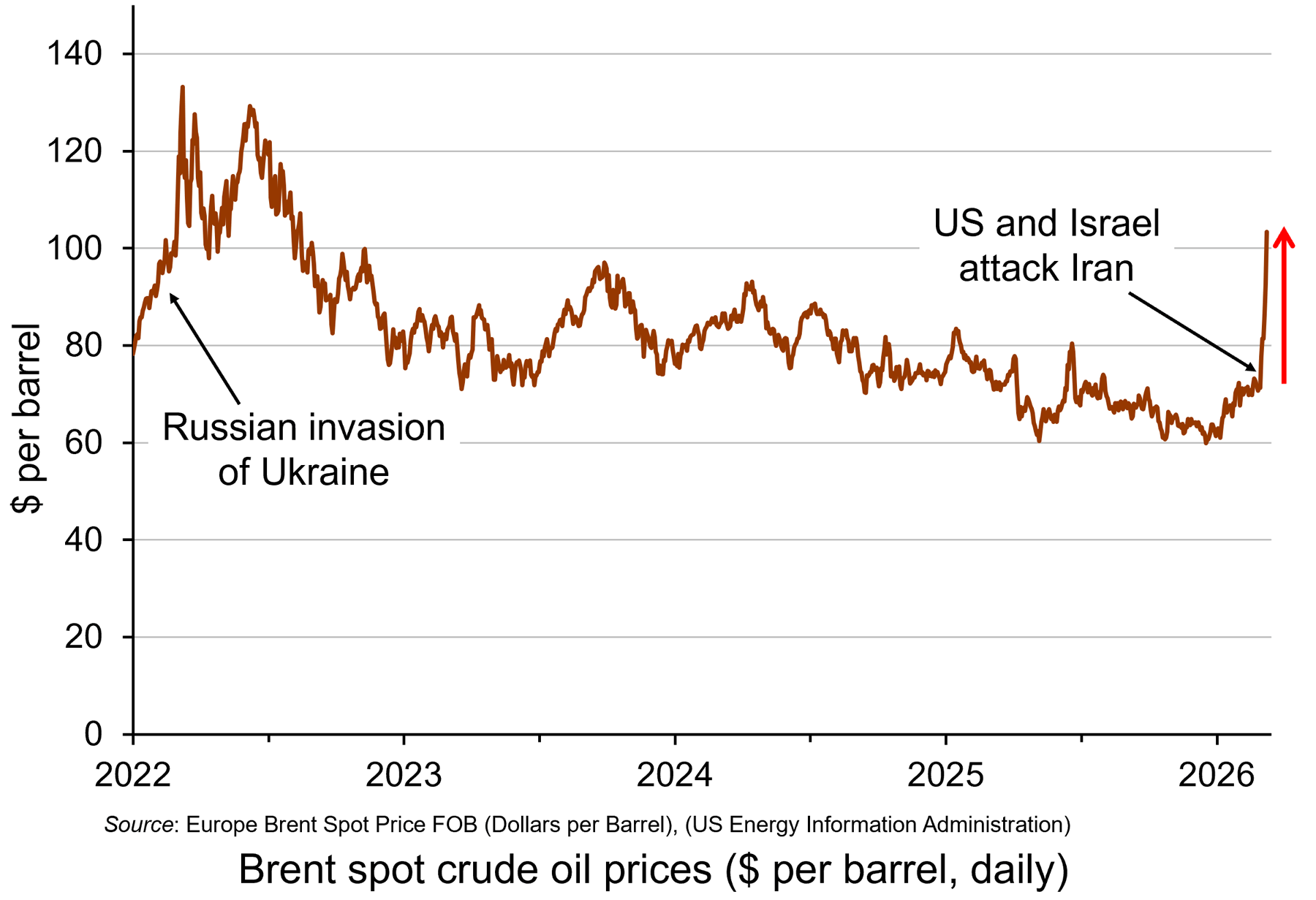
Oil prices rose considerably in the days following the start of the war on 28 February, with Brent crude, a key measure of international oil prices, rising from $71.3 on 27 February to a peak of $119.4 per barrel by the morning of 9 March – a rise of 67%. It was possible that they would rise even further in the short term. However, prices fell back substantially later on 9 March after G7 finance ministers declared that the group ‘stands ready’ to release oil from strategic reserves if needed. By late in the day, the price had fallen to around $90. (Click here for a PowerPoint of the chart.)
However, despite the announcement on 11 March that 32 countries had agreed to release 400m barrels of oil reserves, oil prices began rising again and reached $100 on 12 March after three tankers had been struck in the Gulf, two of them close to the Strait of Hormuz. With Iran pledging to keep the Strait closed, there were worries that the release of oil reserves would provide only temporary relief. Just over 20m barrels of oil normally pass through the Strait of Hormuz. The 400m barrels released from storage is the equivalent, therefore, of only 20 days’ worth of lost oil from the Gulf.
 Rising oil prices will drive up inflation. For those countries with a heavy dependence on Gulf oil, particularly countries in Asia, there could be significant supply problems. For oil exporters in the Persian Gulf, with tankers unable to traverse the Strait of Hormuz, the economic impact is huge. Oil exporters outside the Gulf, such as Russia, Norway and Canada, however, will gain from the higher prices. Clearly the size of these effects will depend on how long the conflict continues and how long the Strait of Hormuz remains closed.
And it is not just oil that is affected. Other products, such as liquified natural gas (LNG), petrochemicals, industrial materials, fertilizers, metals and minerals are transported through the Strait of Hormuz. Gulf countries import much of their food through the Strait.
Cuts in supplies of oil and other products represent an adverse supply shock. Such shocks push up prices (cost-push inflation), while adversely affecting aggregate output. This can lead to stagflation – a combination of higher inflation and stagnation or even falling output. Central banks with a simple mandate to keep inflation to a target are likely to raise interest rates, or at least delay in reducing them. In the USA, with a dual mandate of controlling inflation but also maximising employment, the response may be less deflationary, depending on the judgement of the Federal Reserve.
Uncertainty
 There is great uncertainty about how long the conflict will last. There is also a lack of clarity and consistency from the US administration about its war aims. This uncertainty has affected financial markets, which have seen considerable volatility. Stock markets have seen widespread falls, with airline, travel and AI-heavy stocks being particularly vulnerable.
If the war is concluded relatively swiftly, the economic effects could be relatively small. If the war continues, and especially if the Gulf countries are drawn further into the conflict and if the conflict spreads to other countries, the economic effects could be much more substantial. A prolonged conflict could see oil prices remaining above $100 per barrel, potentially increasing global inflation by 1 percentage point or more. This would slow or halt the move by central banks to cut rates and thereby reduce global economic growth – potentially, as we have seen, leading to stagflation.
Then there is the issue of a potential new international refugee crisis. If the economic and political system in Iran deteriorates rapidly, this could trigger a wave of migration to neighbouring countries, such as Turkey, already hosting large numbers of refugees. Many could seek sanctuary further afield in Europe, with several countries already facing a backlash against immigration. The political and economic effects of this on host countries could be significant – but as yet, highly uncertain.
Articles
- Assessing the global economic impact of the Middle East war
ING, Carsten Brzeski, Warren Patterson, James Knightley and Deepali Bhargava (5/3/26)
- How will the Iran war affect the global economy?
Chatham House, Neil Shearing (6/3/26)
- Iran war is latest threat to a global economy rattled by Trump
Aljazeera, John Power (7/3/26)
- Why an Iran war inflation shock could wreck global economic recovery
The Guardian, Phillip Inman and Kalyeena Makortoff (8/3/26)
- Why has the Iran war sparked fears of stagflation for the global economy?
The Guardian, Luca Ittimani (9/2/26)
- Why surging oil prices are a shock for the global economy – but not yet a crisis
The Conversation, Stella Huangfu (3/3/26)
- Why the price of oil matters more than you might think
BBC News, Natalie Sherman and Mitchell Labiak (10/3/26)
- Strait of Hormuz: Factsheet
IEA (February 2026)
- Strait of Hormuz: Gulf states’ food security is at immediate risk but wider shortages could push up consumer prices globally
The Conversation, Gokcay Balci and Ebru Surucu-Balci (4/3/26)
- Faisal Islam: Oil price spiral may be slowed but not stopped by G7 emergency move
BBC News, Faisal Islam (9/3/26)
- What on earth is going on with the oil price?
BBC News, Jemma Crew (12/3/26)
- Asia scrambles to confront energy crisis unleashed by Iran war – with no end in sight
The Guardian, Callum Jones (12/3/26)
- The grim choice facing the Trump administration: Economic or naval collapse?
CNN, Phil Mattingly and Zachary Cohen (9/3/26)
- How the Iran Conflict May Fuel a New International Refugee Crisis
Forbes, Andy J Semotiuk (5/3/26)
Data
Questions
- Who are the biggest gainers and losers from disruption to oil supplies from the Persian Gulf?
- Illustrate the effect of the current oil price shock on an aggregate demand and supply diagram (either static or dynamic).
- Why is the Iranian war likely to be less damaging to the European economy than the Ukrainian war has been?
- Why have AI-related stock prices been vulnerable to the uncertainty caused by the Iranian war?
- How are the Bank of England and the Federal Reserve Bank likely to respond to the rising price of oil and the broader economic effects of the war? Why might their responses be different?
- What is the likely impact of the Iranian war on global economic recovery?
- How might the Iranian war affect global economic alliances?
- How is the current oil price shock likely to affect the eurozone? Will it be different from the oil price shock that followed the Russian invasion of Ukraine?
- What are the likely economic effects of large-scale migration caused by the war?
 At the fourth anniversary of Russia’s invasion of Ukraine, we look at the effect of the war on the Russian economy. Two years ago, in the blog The Russian economy after two years of war, we argued that the Russian economy had seemingly weathered the war successfully.
Unlike Ukraine, very little of its infrastructure had been destroyed; it had started the war with a current account balance of payments surplus, a budget surplus and a low general government debt-to-GDP ratio; it had achieved a lot of success in diverting its exports, including oil, away from countries imposing sanctions to countries such as China and India; it was the same with imports, with China especially becoming a major suppliers of machinery, components and vehicles; it has a strong central bank, which engenders a high level of confidence in managing inflation; the military expenditure provided a Keynesian boost to the economy, with production and employment rising.
The situation today
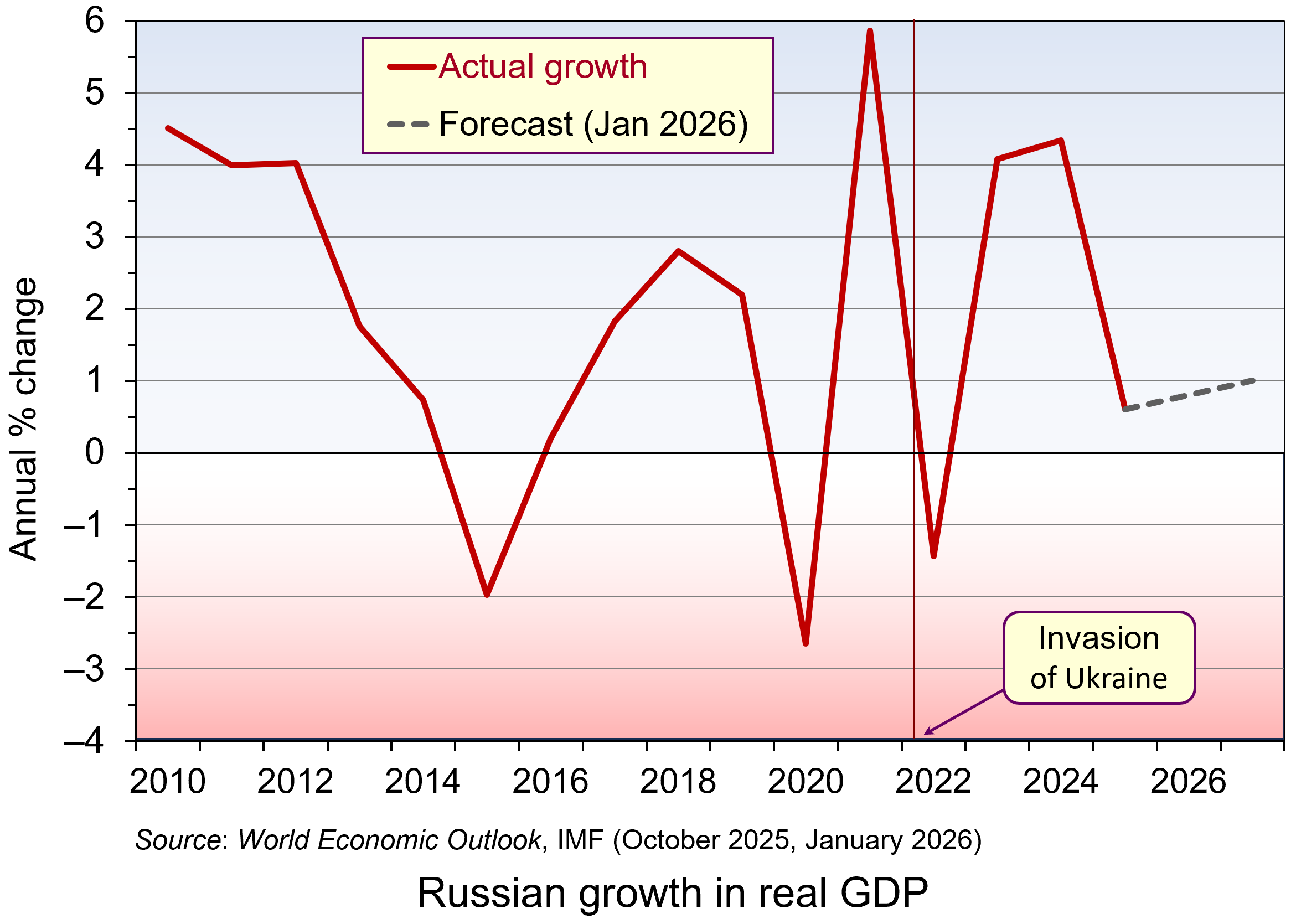 But two years further on, the Russian economy is looking a lot weaker and on the verge of recession. GDP growth fell to 0.6 per cent in 2025 and is forecast to be no more than 1 per cent for the next two years. (Click here for a PowerPoint of the chart.) And despite growth still being positive (just), this is largely because of the growth in military expenditure. Retail and wholesale trade fell by 1.1% in 2025, reflecting supply chain problems and high inflation dampening consumer demand.
With labour being diverted into the armaments and allied industries or into the armed forces, this has led to labour shortages. This has been compounded by the emigration of up to 1 million people by 2025 – often young, educated and skilled professionals.
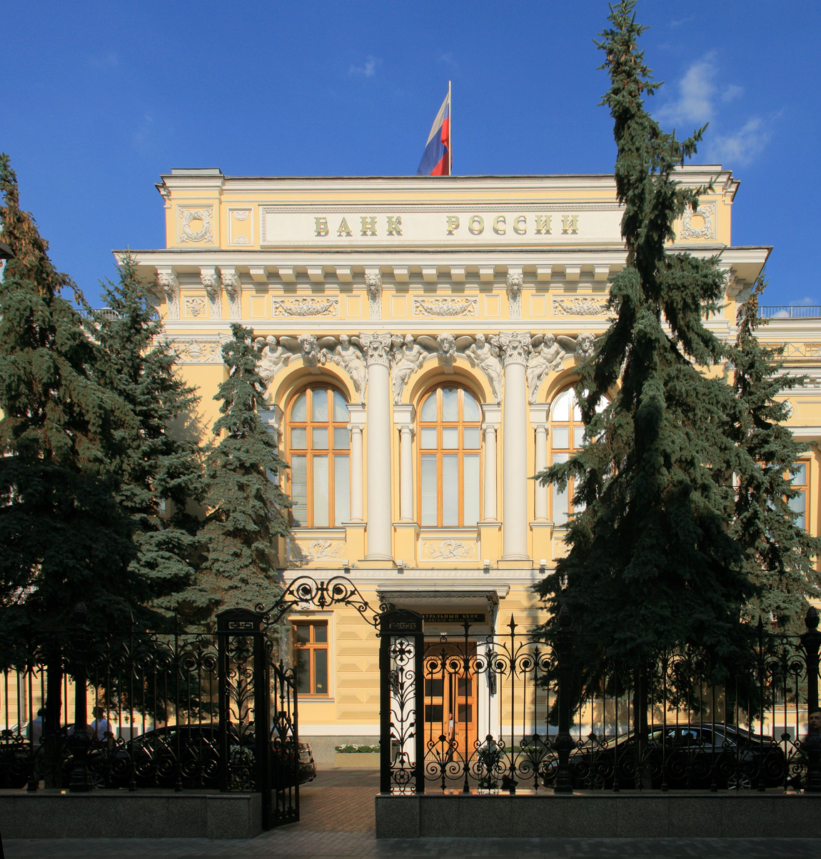 Official CPI inflation averaged 8.7 per cent in 2025, although the prices of food and other consumer essentials rose by more, especially in recent months. At the beginning of 2026, supermarket prices rose by 2.3% in just one month, made worse by a rise in VAT from 20% to 22%. The central bank has responded to the high inflation with high interest rates, which averaged 19.2% in 2025, giving a real rate of 10.5%. With such a high real rate, the response of households has been to save. This has masked the constraints on production, or imports, of consumer goods. Savings have also been boosted by large payments to soldiers and bereaved families, with the money saved by the recipients being used in part to fund future such payments. So far there has been trust in the banking system, but if that trust waned and people starting making large withdrawals of savings, it could be seriously destabilising.
Whilst the high real interest rates have helped to mask shortages of consumer goods, they have had a seriously dampening effect on investment by domestic companies. Gross capital formation fell by 3% in 2025, not helped by an increase in the corporation tax from 20% to 25%. At the same time, foreign direct investment remains subdued due to high perceived risks. The lack of investment, plus the labour shortages, will have profound effects on the supply side of the economy, with potential output in the non-military sector likely to decline over the medium term.
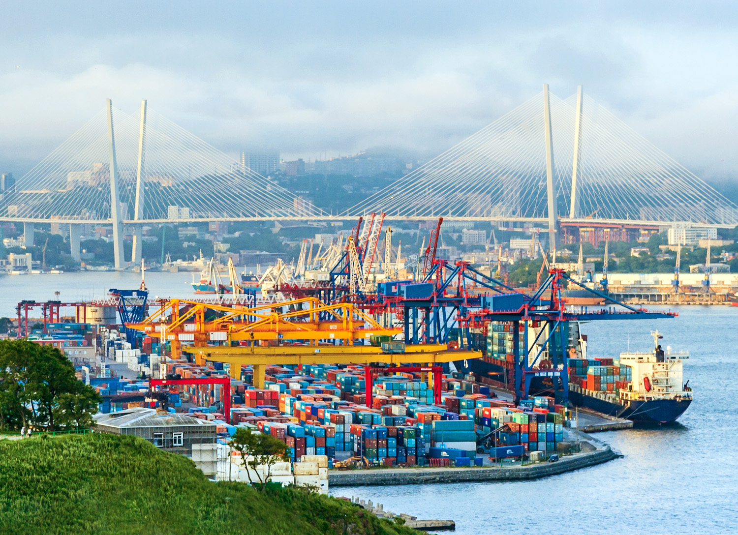 The balance of payments and government finances are turning less favourable. The balance of trade surplus has declined from US$173bn in 2021 to US$67bn in 2025. This could decline further, or even become a deficit, if oil prices continue to be weak, if Western sanctions are tightened (such as stopping the flow of Russian oil exports in the ‘shadow’ fleet of tankers) or if major importing countries stop buying Russian oil. Indian refiners have announced that they are not taking Russian crude in March/April as India seeks to finalise a trade deal with the USA.
The budget balance has moved from a small surplus of 0.8% of GDP in 2021 to a deficit of 2.9% in 2025. Although the government debt-to-GDP ratio remains low by international standards at 23.1% of GDP in 2025, this was up from 16.5% in 2021 and is set to rise further as budget deficits deepen. Nevertheless, as long as the saving rate remains high, the debt can be serviced by domestic bond purchase.
Russia’s economy is definitely weakening and labour shortages and low investment will create major problems for the future. But whether this deterioration will be enough to change Russia’s stance on the war in Ukraine remains to be seen.
Articles
- The Russian economy is finally stagnating. What does it mean for the war – and for Putin?
The Guardian, Alex Clark (6/2/26)
- Exclusive: Russia’s budget deficit may almost triple this year as oil revenues decline
Reuters (4/2/26)
- Russia’s war economy is not collapsing, but neither is it stable
The Conversation, Yerzhan Tokbolat (17/12/25)
- Food prices are surging in Russia. Is the war hitting Russians in the pocket?
BBC News, Olga Shamina, Yaroslava Kiryukhina and Sergei Kagermazov (18/2/26)
- [Russian] GDP data — what it reveals, what it conceals
The Bell, Denis Kasyanchuk (18/2/26)
 What to Expect From the Russian Economy in 2026
Carnegie Endowment for International Peace, Alexandra Prokopenko and Alexander Gabuev (12/2/26)
- Indian refiners avoid Russian oil in push for US trade deal
Reuters, Nidhi Verma (8/2/26)
- What Breaks First – Russia’s Economy or Its War?
Visegrad Insight, Tomasz Kasprowicz (3/2/26)
Videos
Reports
Data
Questions
- What constraints are there currently on the supply side of the Russian economy?
- Some economists have argued that the economic effects of a stalemate in the Ukraine war would suit the Russian leadership more than peace or victory. Why might this be so?
- Under what circumstances might a deep recession in Russia be more likely than stagnation?
- In what ways does Russia’s current financial system resemble a pyramid scheme?
- What cannot a Keynesian boost contunue to support the Russian economy indefinitely?
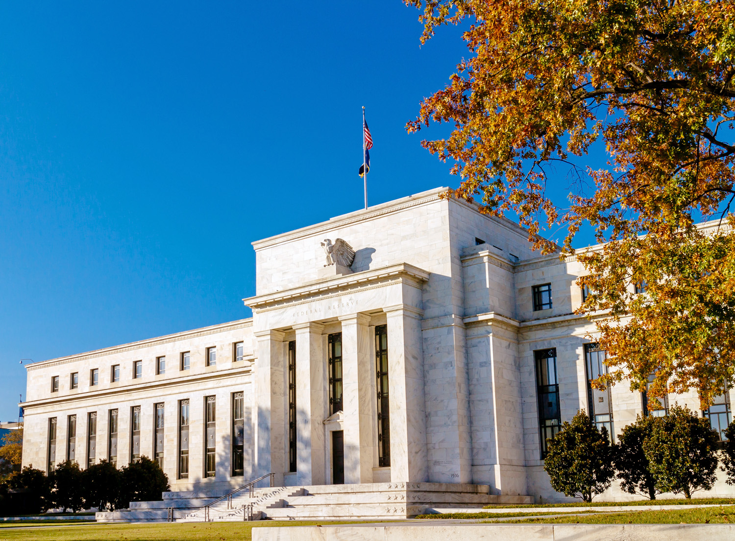 Donald Trump is keen to lower US interest rates substantially and rapidly in order to provide a boost to the US economy. He is also keen to reduce the cost of living for US citizens and sees lower interest rates as a means of reducing the burden of debt servicing for both consumers and firms alike.
But interest rates are set by the US central bank, the Federal Reserve (the ‘Fed’), which is formally independent from government. This independence is seen as important for providing stability to the US economy and removing monetary policy from short-term political pressures to cut interest rates. Succumbing to political pressures would be likely to create uncertainty and damage long-term stability and growth.
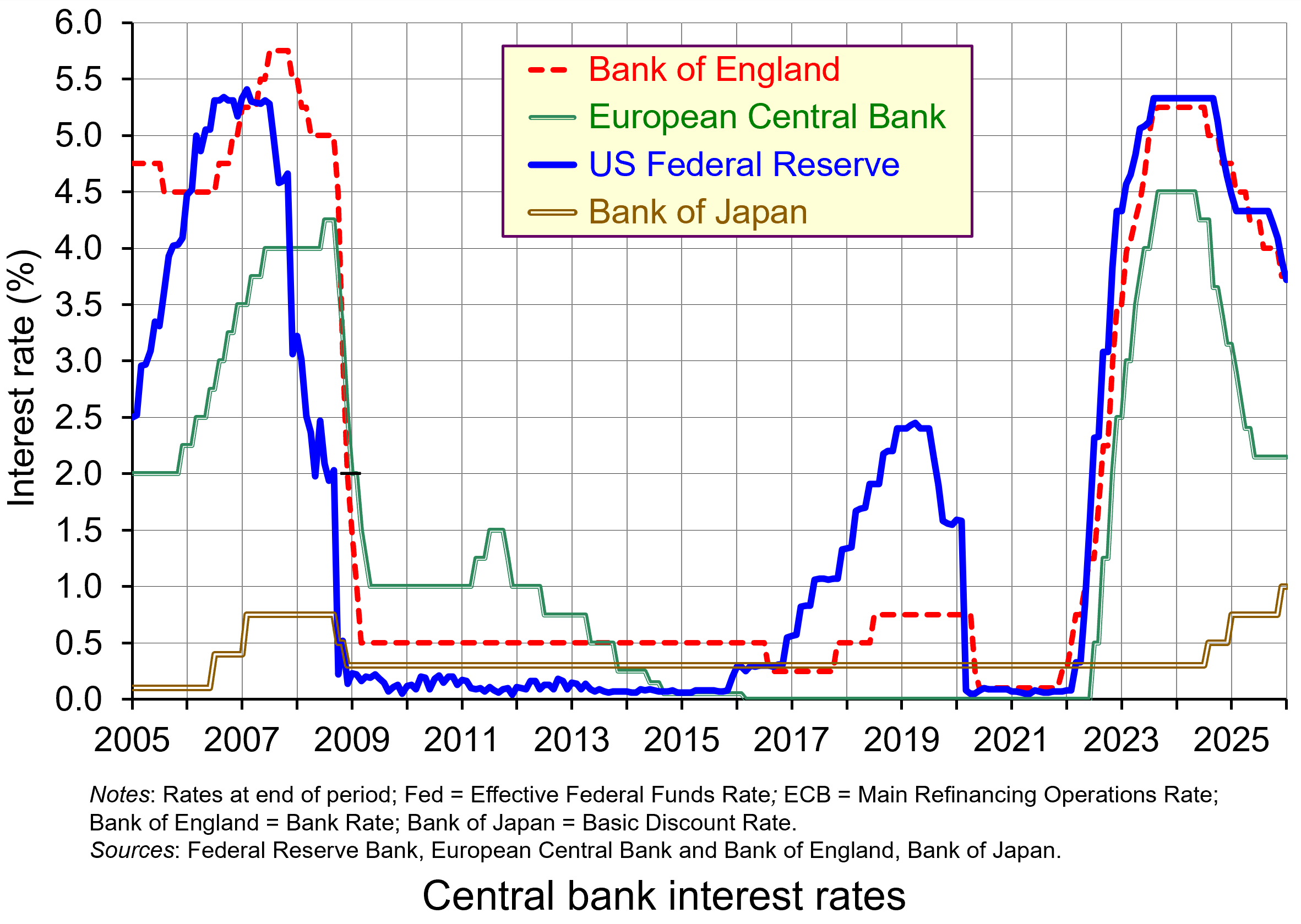
Yet President Trump is pushing the Fed to lower interest rates rapidly and despite three cuts in a row of 0.25 percentage points in the last part of 2025 (see chart below), he thinks this as too little and is annoyed by suggestions that the Fed is unlikely to lower rates again for a while. He has put great pressure on Jerome Powell, the Fed Chair, to go further and faster and has threatened to replace him before his term expires in May this year. He has also made clear that he is likely to appoint someone more willing to cutting rates.
The Federal Reserve headquarters in Washington is currently being renovated. The nine-year project is costing $2.5 billion and is due to be completed next year. President Trump has declared that the project’s costs are excessive and unnecessary.
On 11 January, Federal prosecutors confirmed that they were opening a criminal investigation into Powell, accusing him of lying to Congress in his June 2025 testimony regarding the scope and costs of the renovations.
Powell responded by posting a video in which he claimed that the real reason that he was being threatened with criminal charges was not because of the renovations but because the Fed had ignored President Trump’s pressure and had set interest rates:
based on our best assessment of what will serve the public, rather than following the preferences of the President. This is about whether the Fed will be able to continue to set interest rates based on evidence and economic conditions – or whether, instead, monetary policy will be directed by political pressure or intimidation.
The Fed’s mandate
 The Federal Reserve Board decides on monetary policy and then the Federal Open Market Committee (FOMC) decides how to carry it out. It decides on interest rates and asset sales or purchases. The FOMC meets eight times a year.
The Fed is independent of both the President and Congress, and its Chair is generally regarded as having great power in determining the country’s economic policy.
Since 1977, the Fed’s statutory mandate has been to promote the goals of stable prices and maximum employment. Because of the reference to both prices and employment, the mandate is commonly referred to as a ‘dual mandate’. Its inflation target is 2 per cent over the long run with ‘well anchored’ inflationary expectations.
The dual mandate is unlike that of the Bank of England, the European Central Bank, the Bank of Japan and most other central banks, which all have a single key mandate of achieving a target of a 2 per cent annual rate of consumer price inflation over a particular time period.
With a dual mandate, the two objectives may well conflict from time to time. Moreover, changes in monetary policy affect these objectives with a lag and potentially over different time horizons. Hence, an assessment may have to be made of which is the most pressing problem. This does give some leeway in setting interest rates somewhat lower than if there were a single inflation-rate target. Nevertheless, the assessment is in terms of how best to achieve the mandate and not to meet current political goals.
Statement by former Fed Chairs and Governors
On 12 January, three former Chairs of the Federal Reserve (Janet Yellen, Ben Bernanke and Alan Greenspan), four former Treasury Secretaries (Timothy Geithner, Jacob Lew, Henry Paulson and Robert Rubin) and seven other top former economic officials issued the following statement (see Substack link in the Articles section below):
The Federal Reserve’s independence and the public’s perception of that independence are critical for economic performance, including achieving the goals Congress has set for the Federal Reserve of stable prices, maximum employment, and moderate long-term interest rates. The reported criminal inquiry into Federal Reserve Chair Jay Powell is an unprecedented attempt to use prosecutorial attacks to undermine that independence. This is how monetary policy is made in emerging markets with weak institutions, with highly negative consequences for inflation and the functioning of their economies more broadly. It has no place in the United States whose greatest strength is the rule of law, which is at the foundation of our economic success.
Response of investors
 What will happen to the dollar, US bond prices, share prices and US inflation, and what will happen to investment, depends on how people respond to the threat to the Fed’s independence. Initially, there was little response from markets, with investors probably concluding that President Trump is unlikely to be able to sway FOMC members. What is more, several Republican lawmakers have begun criticising the Trump administration’s criminal investigation, making it harder for the President to influence Fed decisions.
Even if Powell is replaced, either in the short term or in May, by a chair keen to pursue the Trump agenda, that chair will still be just one of twelve voting members of the FOMC.
Seven are appointed by the President, but serve for staggered 14-year terms. Four have been appointed by President Trump, but the other three were appointed by President Biden, although one – Lisa Cook – is being indicted by the Supreme Court for mortgage fraud, with the hearing scheduled for January 21. She claims that this is a trumped-up charge to provide grounds for removing her from the Fed. If she is removed, President Trump could appoint a replacement minded to cut rates.
The other five members include the President of the New York Fed and four of the eleven other regional Fed Presidents serving in rotation. These four are generally hawkish and would oppose early rate cuts.
Thus it is unlikely that President Trump will succeed in pushing the Fed to lower interest rates earlier than they would have done. For that reason, markets have remained relatively sanguine.
 Nevertheless, Donald Trump’s actions could well cause investors to become more worried. Will he try to find other ways to undermine the Fed? Will his actions over Venezuela, Cuba, Greenland and Iran, let alone his policies towards Ukraine and Russia and towards Israel and Gaza, heighten global uncertainty? Will his actions towards Venezuela and his desire to take over Greenland embolden China to attempt to annex Taiwan, and Russia to continue to resist plans to end the war in Ukraine or to make stronger demands?
Such developments could cause investor confidence to wane and for stock markets to fall. Time will tell. I think we need a crystal ball!
Videos
Articles
- Federal prosecutors open criminal investigation into the Fed and Jerome Powell
CNN, Bryan Mena (11/1/26)
- The Fed just gave a rare look at its $2.5 billion renovation — right before Trump’s tour
CNN, Bryan Mena (24/7/25)
- ‘A bone-headed move’: Trump’s shocking battle with Powell could badly backfire
CNN, Matt Egan (12/1/26)
- Why Powell is fighting back against Trump: The US economy is at stake
CNN, Bryan Mena (13/1/26)
- Fed chair Powell hits out at ‘unprecedented’ probe by US justice department
BBC News, Ana Faguy and Osmond Chia (12/1/26)
- Justice department opens investigation into Jerome Powell as Trump ramps up campaign against Federal Reserve
The Guardian, Callum Jones (12/1/26)
- Some Republicans speak out against DoJ investigation into Fed chair
The Guardian, Joseph Gedeon (12/1/26)
- Trump’s attempts to influence Fed risk 1970s-style inflation and global backlash
The Guardian, Richard Partington (12/1/26)
- Statement on the Federal Reserve
Substack, 14 signatories (12/1/26)
- Yellen says Powell probe ‘extremely chilling’ for Fed independence, market should be concerned
CNBC, Jeff Cox (12/1/26)
- Global central bankers unite in defense of Fed Chair Jerome Powell
CNBC, Holly Ellyatt (13/1/26)
- Trump attacks Powell again amid Fed independence fears: ‘That jerk will be gone soon’
CNBC, Kevin Breuninger (13/1/26)
- Former Fed chairs condemn criminal investigation into Jerome Powell
BBC News, Danielle Kaye (12/1/26)
- Fed: Towards a very divided Fed in the coming months and quarters
CPR AM, Bastien Drut (28/11/25)
- Treasury Yields Diverge as Powell Probe Rekindles Fed Independence Risk
Investing.com, Khasay Hashimov (12/1/26)
- Instant View: Investors react as Trump-Fed feud escalates
Reuters (12/1/26)
- Fighting the Fed, Trump tries credit easing by decree
Reuters, Mike Dolan (13/1/26)
- Trump’s attacks on the Federal Reserve risk fuelling US inflation and ending dollar dominance
The Conversation, Emre Tarim (13/1/26)
Questions
- What are the arguments for central bank independence?
- What are the arguments for control of monetary policy by the central government?
- Assess the above arguments.
- Find out what has happened to interest rates, the US stock market and the dollar since this blog was written.
- How do the fiscal decisions by government affect monetary policy?
- Compare the benefits of the dual mandate system of the Fed with those of the single mandate of the Bank of England and ECB.
 The following blog is inspired by my teaching of macroeconomic issues to my final year students at Aston University. In the classes we’ve been discussing important aspects of monetary and fiscal policy design. What has become clear to me and my students is that the trade-offs which characterise the discipline of economics are certainly alive and well in the current environment in which monetary and fiscal policy choices are being made.
To demonstrate this we consider here some of the discussions we’ve had in class around central bank independence and monetary policy mandates. We’ve also looked at fiscal policy. Here we’ve examined the state of the public finances and the importance that seems to be attached to debt stabilisation and the imposition of debt rules.
Delegation and central bank mandates
My teaching this term began by introducing my students to one of the most important and influential monetary policy models. This is the model of Kydland and Prescott. Their model, published in the Journal of Political Economy in 1977 has become the theoretical bedrock for the modern-day operational independence of central banks.1
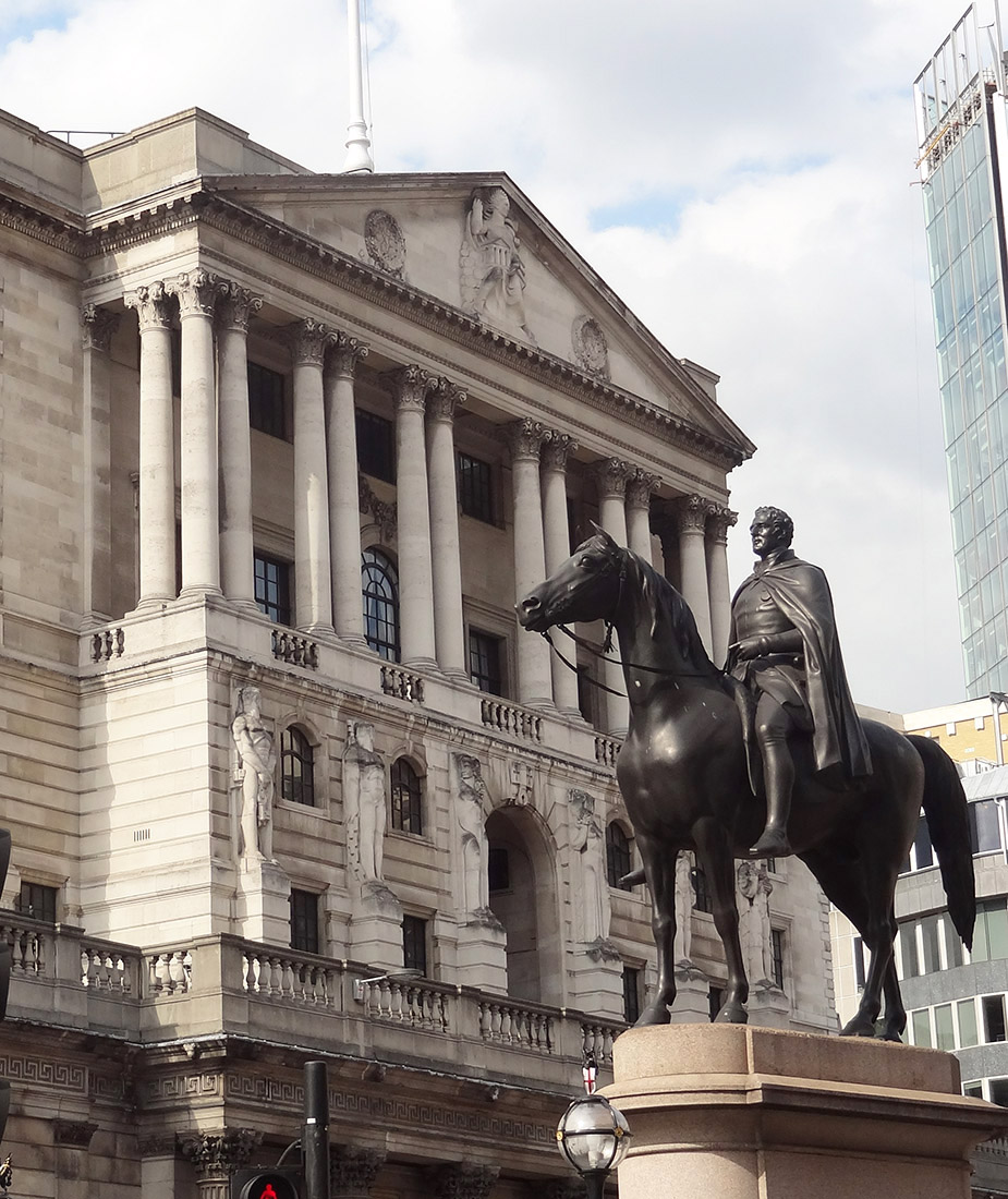 The model explores how systemically high inflation can become established in economies when policymakers have the political incentive to lower unemployment or increase output above its long-run equilibrium value. This may be the case if governments operate monetary policy rather than the central bank (of if the central bank operates monetary policy but follows government objectives). By adopting expansionary monetary policy, governments can increase their popularity.
But this is likely to be short-lived, as any increased economic activity will only be temporary (assuming that the natural-rate hypothesis holds). Soon, inflation will rise.
But, if an election is on the horizon, there may be enough time to boost output and employment before inflation rises. In other words, an expectations-augmented Phillips curve may present governments with an incentive to loosen monetary policy and worry about the inflation consequences after the election.
However, the resulting ‘inflation surprise’ through the loosening of monetary policy means a fall in real pay and therefore in purchasing power. If people suspect that governments will be tempted to loosen policy, they will keep their expectations of inflation higher than the socially optimal inflation rate. Consequently, low-inflation targets lack credibility when governments have the temptation to loosen monetary policy. Such targets are time-inconsistent because governments have an incentive to renege and deliver higher inflation through a looser monetary policy. The result is an inflation bias.
Central bank independence
To prevent this inflationary bias arising, many central banks around the world have been given some form of operational independence with a mandate centred around an inflation-rate target. By delegating monetary policy to a more conservative central bank, the problem of inflationary bias can be addressed.
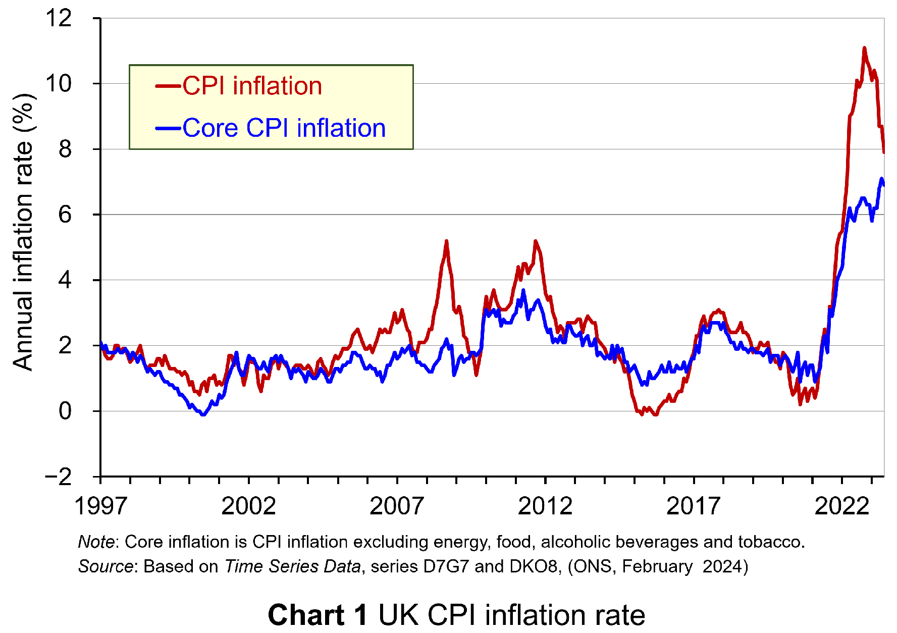 Yet central bank independence is not without its own issues and this has been an important part of the discussions with my students. Today, many economies are continuing to experience the effects of the inflationary shocks that began in 2021 (see Chart 1 for the UK CPI inflation rate: click here for a PowerPoint). The question is whether the appointment of a conservative or hard-nosed hawkish central banker trades off the stabilisation of inflation for greater volatility in output or unemployment.
The inflation–output stabilisation trade-off is closely associated with the works of Kenneth Rogoff2 and John Taylor3. The latter is known for his monetary policy rule, which has become known as the ‘Taylor rule’. This advocates that a rules-based central bank ought to place weight on both inflation and output stabilisation.
This is not without its own issues, however, since, by also placing weight on output stabilisation, we are again introducing the possibility of greater inflationary bias in policy making. Hence, while the act of delegation and a rules- or target-based approach may mitigate the extent of the bias relative to that in the Kydland and Prescott model, there nonetheless still remain issues around the design of the optimal framework for the conduct of monetary policy.
Indeed, the announcement that the UK had moved into recession in the last two quarters of 2023 can be seen as evidence that an otherwise abstract theoretical trade-off between inflation and output stabilisation is actually very real.
My classroom discussions have also shown how economic theory struggles to identify an optimal inflation-rate target. Beyond accepting that a low and stable inflation rate is desirable, it is difficult to address fully the student who asks what is so special about a 2% inflation target. Would not a 3% target, for example, be preferable, they might ask?
Whilst this may sound somewhat trivial, it has real-world consequences. In a world that now seems to be characterised by greater supply-side volatility and by more frequent inflation shocks than we were used to in recent history, might a higher inflation rate target be preferable? Certainly, one could argue that, with an inflation–output stabilisation trade-off, there is the possibility that monetary policy could be unduly restrictive in our potential new macroeconomic reality. Hence, we might come to see governments and central banks in the near future revisiting the mandates that frame the operation of their monetary policy. Time will tell.
Fiscal policy and debt stabilisation
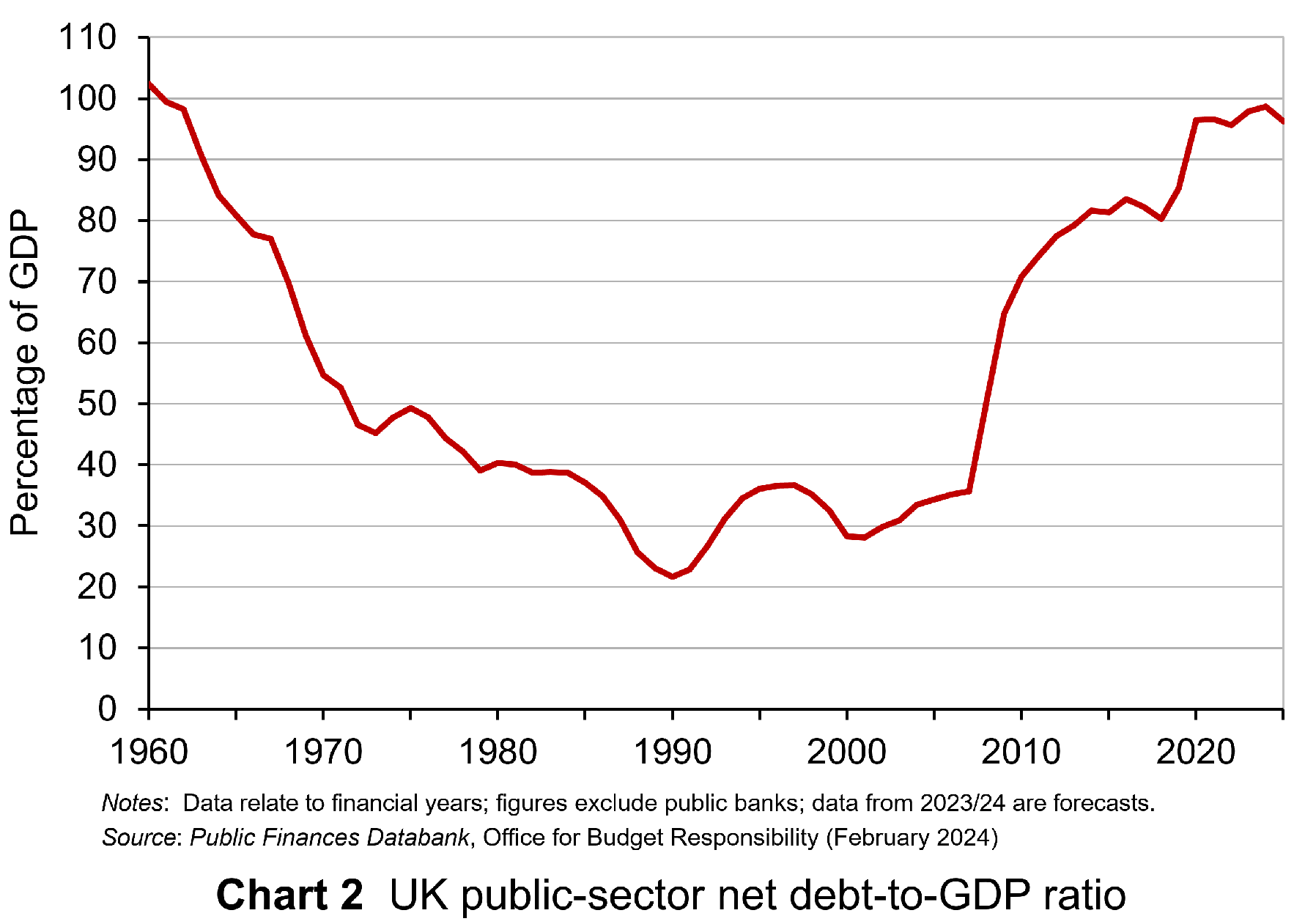 The second topic area that I have been discussing in my final-year macroeconomics classes has centred around fiscal policy and the state of the public finances. The context for this is that we have seen a significant increase in public debt-to-GDP ratios over the past couple of decades as the public sector has attempted to absorb significant economic shocks. These include the global financial crisis of 2007–8, the COVID-19 pandemic and the cost-of-living crisis. These interventions in the case of the UK have seen its public debt-to-GDP ratio more than triple since the early 2000s to close to 100% (see Chart 2: click here for a PowerPoint).
Understandably, given the stresses placed on the public finances, economists have increasingly debated issues around debt sustainability. These debates have been mirrored by politicians and policymakers. A key question is whether to have a public debt rule. The UK has in recent years adopted such a rule. The arguments for a rule centre on ensuring sound public finances and maintaining the confidence of investors to purchases public debt. A debt rule therefore places a discipline on fiscal policy, with implications for taxation and spending.
How easy it is to stick to a debt rule depends on three key factors. It will be harder to stick to the rule:
- The higher the current debt-to-GDP ratio and hence the more it needs to be reduced to meet the rule.
- The higher the rate of interest and hence the greater the cost of servicing the public debt.
- The lower the rate of economic growth and hence the less quickly will tax revenues rise.
With a given debt-to-GDP ratio, a given average interest rate payable on its debt, and a given rate of economic growth, we can determine the primary fiscal balance relative to GDP a government would need to meet for the debt-to-GDP ratio to remain stable. This is known as the ‘debt-stabilising primary balance’. The primary balance is the difference between a government’s receipts and its expenditures less the interest payments on its debt.
 This fiscal arithmetic is important in determining a government’s fiscal choices. It shows the implications for spending and taxation. These implications become ever more important and impactful on people, businesses, and society when the fiscal arithmetic becomes less favourable. This is a situation that appears to be increasingly the case for many countries, including the UK, as the rate of interest on public debt rises relative to a country’s rate of economic growth. As this happens, governments are increasingly required to run healthier primary balances. This of course implies a tightening of their fiscal stance.
Hence, the fiscal conversations with my students have focused on both the benefits and the costs of debt-stabilisation. In respect of the costs, a few issues have arisen.
First, as with the inflation-rate target, it is hard to identify an optimal public debt-to-GDP ratio number. While the fiscal arithmetic may offer some clue, it is not straightforward to address the question as to whether a debt-to-GDP ratio of say 100% or 120% would be excessive for the UK.
Second, it is possible that the debt stabilisation itself can make the fiscal arithmetic of debt stabilisation more difficult. This occurs if fiscal consolidation itself hinders long-term economic growth, which then makes the fiscal arithmetic more difficult. This again points to the difficulties in designing policy frameworks, whether they be for monetary or fiscal policy.
Third, a focus on debt stabilisation alone ignores the fact that there are two sides to any sector’s balance sheet. It would be very unusual when assessing the well-being of businesses or households if we were to ignore the asset side of their balance sheet. Yet, this is precisely the danger of focusing on public debt at the exclusion of what fiscal choices can mean for public-sector assets, from which we all can potentially benefit. Hence, some would suggest a more balanced approach to assessing the soundness of the public finances might involve a net worth (assets less liabilities) measure. This has parallels with the debates around whether mandates of central banks should be broader.
Applications in macroeconomics
What my teaching of a topics-based macroeconomics module this term has vividly demonstrated is that concepts, theories, and models come alive, and are capable of being understood better, when they are used to shine a light on real-world issues. The light being shone on monetary and fiscal policy in today’s turbulent macroeconomic environment is perhaps understandably very bright.
Indeed, the light being shone on fiscal policy in the UK and some other countries facing an upcoming election, is intensified further with the state of the public finances shaping much of the public discourse on fiscal choices. Hopefully, my students will continue to debate these important issues beyond their graduation, stressing their importance for people’s lives and, in doing so, going beyond the abstract.
References
- Rules rather than discretion: The inconsistency of optimal plans
The Journal of Political Economy, Finn E Kydland and Edward C. Prescott (1977, 85(3), pp 473–92)
- The optimal degree of commitment to an intermediate monetary target
Quarterly Journal of Economics, Kenneth Rogoff (November 1985, 100(4), pp 1169–89)
- Discretion versus policy rules in practice
Carnegie-Rochester Conference Series on Public Policy, John B Taylor (December 1993, 39, pp 195–214)
Articles
Questions
- What is meant by time-inconsistent monetary policy announcements? How has this concept been important for the way in which many central banks now conduct monetary policy?
- What is meant by a ‘conservative’ central banker? Why is the appointment of this type of central banker thought to be important in affecting inflation?
- What is the contemporary macroeconomic relevance of the inflation–output (or inflation–unemployment) stabilisation trade-off?
- How is the primary balance different from the actual budget balance?
- What do you understand by the concept of ‘the fiscal arithmetic’. Explain how each element of the fiscal arithmetic affects the debt-stabilising primary balance?
- Analyse the costs of benefits of a debt-based fiscal rule.
 It’s two years since Russia invaded Ukraine. Western countries responded by imposing large-scale sanctions. These targeted a range of businesses, banks and other financial institutions, payments systems and Russian exports and imports. Some $1 trillion of Russian assets were frozen. Many Western businesses withdrew from Russia or cut off commercial ties. In addition, oil and gas imports from Russia have been banned by most developed countries and some developing countries, and a price cap of $60 per barrel has been imposed on Russian oil. What is more, sanctions have been progressively tightened over the past two years. For example, on the second anniversary of the invasion, President Biden announced more than 500 new sanctions against individuals and companies involved in military production and supply chains and in financing Russia’s war effort.
The economy in Russia has also been affected by large-scale emigration of skilled workers, the diversion of workers to the armed forces and the diversion of capital and workers to the armaments industry.
So has the economy of Russia been badly affected by sanctions and these other factors? The IMF in its World Economic Forecast of April 2022 predicted that the Russian economy would experience a steep, two-year recession. But, the Russian economy has fared much better than first predicted and the steep recession never materialised.
In this blog we look at Russia’s economic performance. First, we examine why the Russian economy seems stronger today than forecast two years ago. Then we look at its economic weaknesses directly attributable to the war.
Apparent resilience of the Russian economy
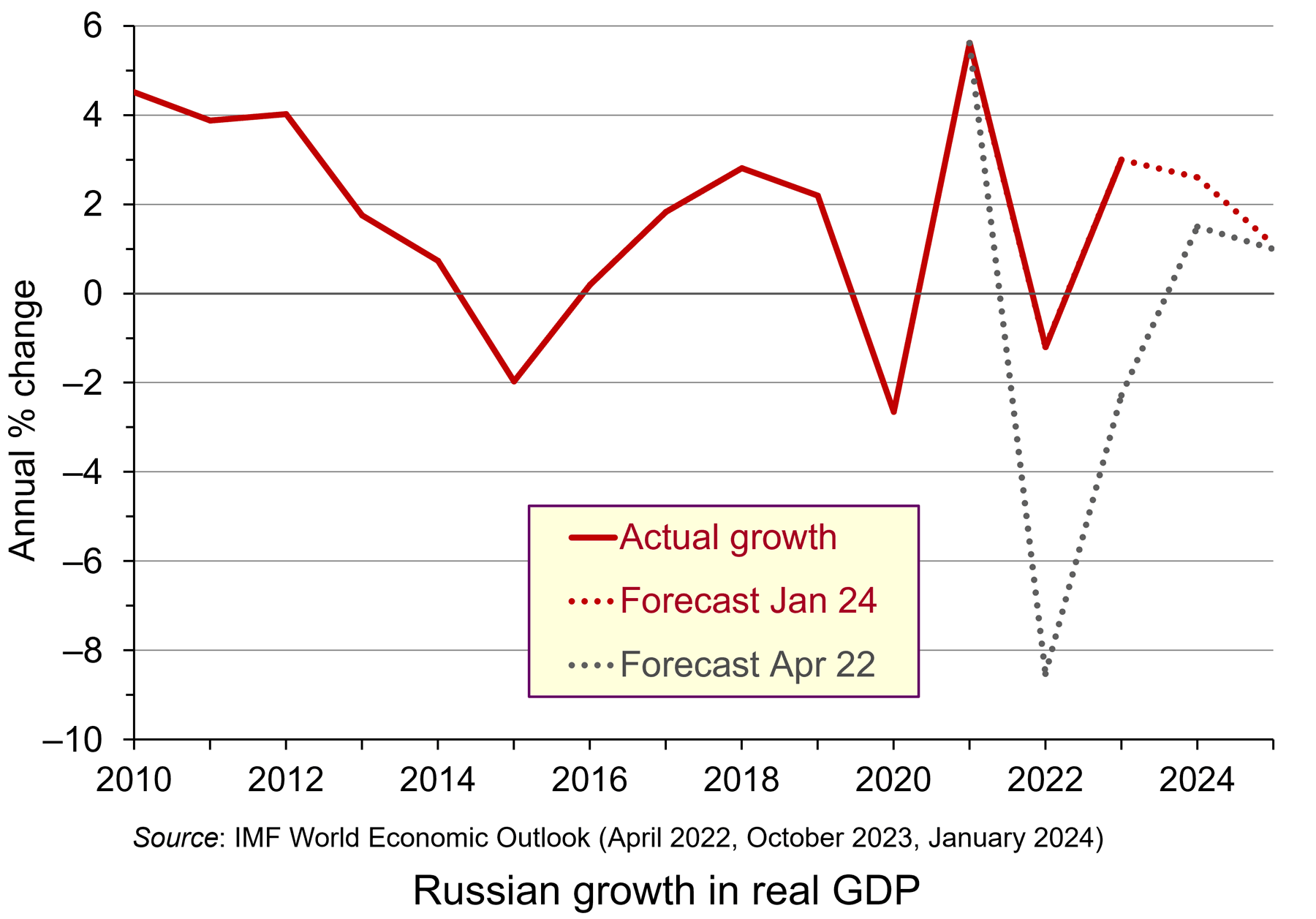 GDP forecasts have proved wrong. In April 2022, just after the start of the war, the IMF was forecasting that the Russian economy would decline by 8.5% in 2022 and by 2.3% in 2023 and grow by just 1.5% in 2024. In practice, the economy declined by only 1.2% in 2022 and grew by 3.0% in 2023. It is forecast by the IMF to grow by 2.6% in 2024. This is illustrated in the chart (click here for a PowerPoint).
Similarly, inflation forecasts have proved wrong. In April 2022, Russian consumer price inflation was forecast to be 21.3% in 2022 and 14.3% in 2023. In practice, inflation was 13.8% in 2022 and 7.4% in 2023. What is more, consumer spending in Russia has remained buoyant. In 2023, retail sales rose by 10.2% in nominal terms – a real rise of 2.8%. Wage growth has been strong and unemployment has remained low, falling from just over 4% in February 2022 to just under 3% today.
So why has the Russian economy seemingly weathered the war so successfully?
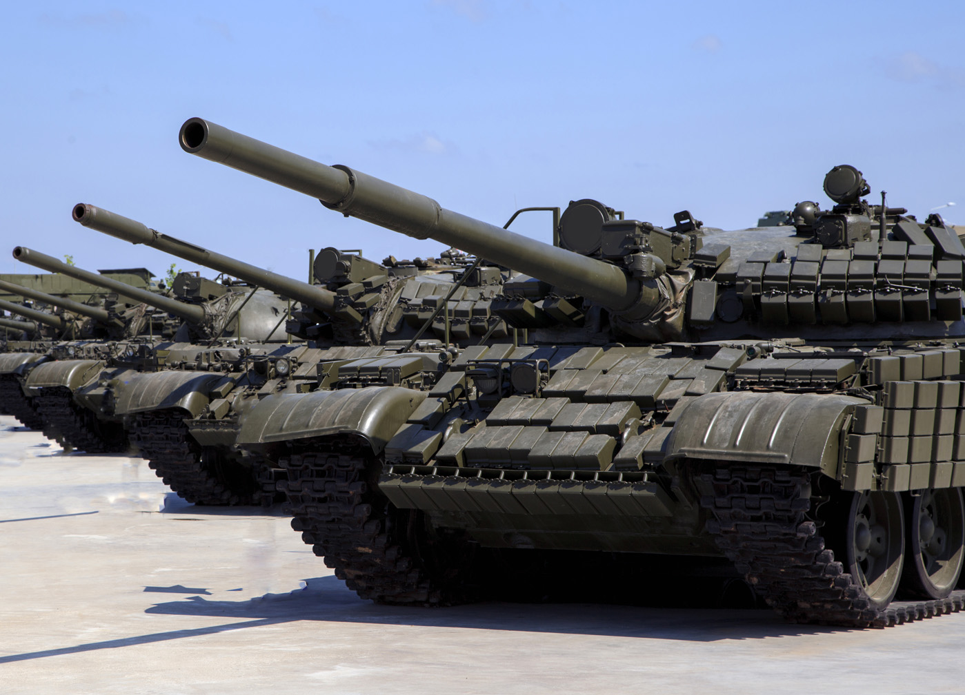 The first reason is that, unlike Ukraine, very little of its infrastructure has been destroyed. Even though it has lost a lot of its military capital, including 1120 main battle tanks and some 2000 other armoured vehicles, virtually all of its production capacity remains intact. What is more, military production is replacing much of the destroyed vehicles and equipment.
The second is that its economy started the war in a strong position economically. In 2021, it had a surplus on the current account of its balance of payments of 6.7% of GDP, reflecting large revenues from oil, gas and mineral exports. This compares with a G7 average deficit of 0.7%. It had fiscal surplus (net general government lending) of 0.8% of GDP. The G7 countries had an average deficit of 9.1% of GDP. Its gross general government debt was 16% of GDP. The G7’s was an average of 134%. This put Russia in a position to finance the war and gave it a considerable buffer against economic sanctions.
 The third reason is that Russia has been effective in switching the destinations of exports and sources of imports. Trade with the West, Japan and South Korea has declined, but trade with China and various neutral countries, such as India have rapidly increased. Take the case of oil: in 2021, Russia exported 4.4 billion barrels of oil per day to the USA, the EU, the UK, Japan and South Korea. By 2023, this had fallen to just 0.6 billion barrels. By contrast, in 2021, it exported 1.9 billion barrels per day to China, India and Turkey. By 2023, this had risen to 4.9 billion. Although exports of natural gas have fallen by around 42% since 2021, Russian oil exports have remained much the same at around 7.4 million barrels per day (until a voluntary cut of 0.5 billion barrels per day in 2024 Q1 as part of an OPEC+ agreement to prop up the price of oil).
China is now a major supplier to Russia of components (some with military uses), commercial vehicles and consumer products (such as cars and electrical goods). Total trade with China (both imports and exports) was worth $147 billion in 2021. By 2023, this had risen to $240 billion.
The use of both the Chinese yuan and the Russian rouble (or ruble) has risen dramatically as a means of payment for Russian imports. Their share has risen from around 5% in 2021 (mainly roubles) to nearly 75% in 2023 (just over 37% in each currency). Switching trade and payment methods has helped Russia to circumvent many of the sanctions.
 The fourth reason is that Russia has a strong and effective central bank. It has successfully used interest rates to control inflation, which is expected to fall from 7.4% in 2023 to under 5% this year and then to its target of 4% in subsequent years. The central bank policy rate was raised from 8.5% to 20% in February 2022. It then fell in steps to 7.5% in September 2022, where it remained until August 2023. It was then raised in steps to peak at 16% in December 2023, where it remains. There is a high level of confidence that the Russian central bank will succeed in bringing inflation back to target.
The fifth reason is that the war has provided a Keynesian stimulus to the economy. Military expenditure has doubled as a share of GDP – from 3.7% of GDP in 2021 to 7.5% in 2024. It now accounts for around 40% of government expenditure. The boost that this has given to production and employment has helped achieve the 3% growth rate in 2023, despite the dampening effect of a tight monetary policy.
Longer-term weaknesses
Despite the apparent resilience of the economy, there are serious weaknesses that are likely to have serious long-term effects.
There has been a huge decline in the labour supply as many skilled and professional workers have move abroad to escape the draft and as many people have been killed in battle. The shortage of workers has led to a rise in wages. This has been accompanied by a decline in labour productivity, which is estimated to have been around 3.6% in 2023.
 Higher wages and lower productivity is putting a squeeze on firms’ profits. This is being exacerbated by higher taxes on firms to help fund the war. Lower profit reduces investment and is likely to have further detrimental effects on labour productivity.
Although Russia has managed to circumvent many of the sanctions, they have still had a significant effect on the supply of goods and components from the West. As sanctions are tightened further, so this is likely to have a direct effect on production and living standards. Although GDP is growing, non-military production is declining.
The public finances at the start of the war, as we saw above, were strong. But the war effort has turned a budget surplus of 0.8% of GDP in 2021 to a deficit of 3.7% in 2023 – a deficit that will be difficult to fund with limited access to foreign finance and with domestic interest rates at 16%. As public expenditure on the military has increased, civilian expenditure has decreased. Benefits and expenditure on infrastructure are being squeezed. For example, public utilities and apartment blocks are deteriorating badly. This has a direct on living standards.
In terms of exports, although by diverting oil exports to China, India and other neutral countries Russia has manage to maintain the volume of its oil exports, revenue from them is declining. Oil prices have fallen from a peak of $125 per barrel in June 2022 to around $80 today. Production from the Arabian Gulf is likely to increase over the coming months, which will further depress oil prices.
Conclusions
With the war sustaining the Russian economy, it would be a problem for Russia if the war ended. If Russia won by taking more territory in Ukraine and forcing Ukraine to accept Russia’s terms for peace, the cost to Russia of rebuilding the occupied territories would be huge. If Russia lost territory and negotiated a settlement on Ukraine’s terms, the political cost would be huge, with a disillusioned Russian people facing reduced living standards that could lead to the overthrow of Putin. As The Conversation article linked below states:
A protracted stalemate might be the only solution for Russia to avoid total economic collapse. Having transformed the little industry it had to focus on the war effort, and with a labour shortage problem worsened by hundreds of thousands of war casualties and a massive brain drain, the country would struggle to find a new direction.
Articles
- How Russia’s economy survived two years of war
The Bell (23/2/24)
- How Russia uses China to get round sanctions
The Bell, Denis Kasyanchuk (20/2/24)
- As Ukraine’s economy burns, Russia clings to a semblance of prosperity
The Observer, Larry Elliott and Phillip Inman (24/2/24)
- ‘A lot higher than we expected’: Russian arms production worries Europe’s war planners
The Guardian, Andrew Roth (15/2/24)
- There are lessons from Russia’s GDP growth — but not the ones Putin thinks
Financial Times, Martin Sandbu (11/2/24)
 Russia’s economy going strong
DW, Miltiades Schmidt (21/2/24)
- The West tried to crush Russia’s economy. Why hasn’t it worked?
Politico, Nahal Toosi, Ari Hawkins, Koen Verhelst, Gabriel Gavin and Kyle Duggan (24/2/24)
- Don’t Buy Putin’s Bluff. The West Can Outspend Him.
Bloomberg UK, Editorial (23/2/24)
- Russia’s war economy cannot last but has bought time
BBC News, Faisal Islam (11/2/24)
- US targets Russia with more than 500 new sanctions
BBC News, George Wright and Will Vernon (24/2/24)
- Russia’s economy is now completely driven by the war in Ukraine – it cannot afford to lose, but nor can it afford to win
The Conversation, Renaud Foucart (22/2/24)
Questions
- Argue the case for and against including military production in GDP.
- How successful has the freezing of Russian assets been?
- How could Western sanctions against Russia be made more effective?
- What are the dangers to Western economies of further tightening financial sanctions against Russia?
- Would it be a desirable policy for a Western economy to divert large amounts of resources to building public infrastructure?
- Has the Ukraine war hastened the rise of the Chinese yuan as a reserve currency?
- How would you summarise Russia’s current public finances?
- How would you set about estimating the cost to Russia of its war with Ukraine?
 With relentless bombing of Iran by Israel and the USA, and with Iranian counterattacks on Gulf states, the costs of the war are mounting. The most obvious are in terms of human lives, injuries and suffering. But there are significant economic costs too. Some of these are immediate, such as the rising price of oil and hence the costs of fuel, or the fall in stock market prices. Some will be longer term, depending on how the war develops. For example, prices could rise more generally as supply chains are disrupted.
 The impacts will vary across the world and across markets. The most obvious markets to be affected are those where significant supply comes from the Persian Gulf. Approximately 20% of total global oil consumption passes through the Strait of Hormuz, which connects the Persian Gulf with the Arabian Sea and the Indian Ocean.
 Rising oil prices will drive up inflation. For those countries with a heavy dependence on Gulf oil, particularly countries in Asia, there could be significant supply problems. For oil exporters in the Persian Gulf, with tankers unable to traverse the Strait of Hormuz, the economic impact is huge. Oil exporters outside the Gulf, such as Russia, Norway and Canada, however, will gain from the higher prices. Clearly the size of these effects will depend on how long the conflict continues and how long the Strait of Hormuz remains closed.
 There is great uncertainty about how long the conflict will last. There is also a lack of clarity and consistency from the US administration about its war aims. This uncertainty has affected financial markets, which have seen considerable volatility. Stock markets have seen widespread falls, with airline, travel and AI-heavy stocks being particularly vulnerable.
 At the fourth anniversary of Russia’s invasion of Ukraine, we look at the effect of the war on the Russian economy. Two years ago, in the blog
  But two years further on, the Russian economy is looking a lot weaker and on the verge of recession. GDP growth fell to 0.6 per cent in 2025 and is forecast to be no more than 1 per cent for the next two years. (Click
  Official CPI inflation averaged 8.7 per cent in 2025, although the prices of food and other consumer essentials rose by more, especially in recent months. At the beginning of 2026, supermarket prices rose by 2.3% in just one month, made worse by a rise in VAT from 20% to 22%. The central bank has responded to the high inflation with high interest rates, which averaged 19.2% in 2025, giving a real rate of 10.5%. With such a high real rate, the response of households has been to save. This has masked the constraints on production, or imports, of consumer goods. Savings have also been boosted by large payments to soldiers and bereaved families, with the money saved by the recipients being used in part to fund future such payments. So far there has been trust in the banking system, but if that trust waned and people starting making large withdrawals of savings, it could be seriously destabilising.
 The balance of payments and government finances are turning less favourable. The balance of trade surplus has declined from US$173bn in 2021 to US$67bn in 2025. This could decline further, or even become a deficit, if oil prices continue to be weak, if Western sanctions are tightened (such as stopping the flow of Russian oil exports in the ‘shadow’ fleet of tankers) or if major importing countries stop buying Russian oil. Indian refiners have announced that they are not taking Russian crude in March/April as India seeks to finalise a trade deal with the USA.
 Donald Trump is keen to lower US interest rates substantially and rapidly in order to provide a boost to the US economy. He is also keen to reduce the cost of living for US citizens and sees lower interest rates as a means of reducing the burden of debt servicing for both consumers and firms alike.
 The Federal Reserve Board decides on monetary policy and then the Federal Open Market Committee (FOMC) decides how to carry it out. It decides on interest rates and asset sales or purchases. The FOMC meets eight times a year.
  What will happen to the dollar, US bond prices, share prices and US inflation, and what will happen to investment, depends on how people respond to the threat to the Fed’s independence. Initially, there was little response from markets, with investors probably concluding that President Trump is unlikely to be able to sway FOMC members. What is more, several Republican lawmakers have begun criticising the Trump administration’s criminal investigation, making it harder for the President to influence Fed decisions.
 Nevertheless, Donald Trump’s actions could well cause investors to become more worried. Will he try to find other ways to undermine the Fed? Will his actions over Venezuela, Cuba, Greenland and Iran, let alone his policies towards Ukraine and Russia and towards Israel and Gaza, heighten global uncertainty? Will his actions towards Venezuela and his desire to take over Greenland embolden China to attempt to annex Taiwan, and Russia to continue to resist plans to end the war in Ukraine or to make stronger demands?
 The following blog is inspired by my teaching of macroeconomic issues to my final year students at Aston University. In the classes we’ve been discussing important aspects of monetary and fiscal policy design. What has become clear to me and my students is that the trade-offs which characterise the discipline of economics are certainly alive and well in the current environment in which monetary and fiscal policy choices are being made.
 The model explores how systemically high inflation can become established in economies when policymakers have the political incentive to lower unemployment or increase output above its long-run equilibrium value. This may be the case if governments operate monetary policy rather than the central bank (of if the central bank operates monetary policy but follows government objectives). By adopting expansionary monetary policy, governments can increase their popularity.
 Yet central bank independence is not without its own issues and this has been an important part of the discussions with my students. Today, many economies are continuing to experience the effects of the inflationary shocks that began in 2021 (see Chart 1 for the UK CPI inflation rate: click
  The second topic area that I have been discussing in my final-year macroeconomics classes has centred around fiscal policy and the state of the public finances. The context for this is that we have seen a significant increase in public debt-to-GDP ratios over the past couple of decades as the public sector has attempted to absorb significant economic shocks. These include the global financial crisis of 2007–8, the COVID-19 pandemic and the cost-of-living crisis. These interventions in the case of the UK have seen its public debt-to-GDP ratio more than triple since the early 2000s to close to 100% (see Chart 2: click
  This fiscal arithmetic is important in determining a government’s fiscal choices. It shows the implications for spending and taxation. These implications become ever more important and impactful on people, businesses, and society when the fiscal arithmetic becomes less favourable. This is a situation that appears to be increasingly the case for many countries, including the UK, as the rate of interest on public debt rises relative to a country’s rate of economic growth. As this happens, governments are increasingly required to run healthier primary balances. This of course implies a tightening of their fiscal stance.
 GDP forecasts have proved wrong. In April 2022, just after the start of the war, the IMF was forecasting that the Russian economy would decline by 8.5% in 2022 and by 2.3% in 2023 and grow by just 1.5% in 2024. In practice, the economy declined by only 1.2% in 2022 and grew by 3.0% in 2023. It is forecast by the IMF to grow by 2.6% in 2024. This is illustrated in the chart (click
  The first reason is that, unlike Ukraine, very little of its infrastructure has been destroyed. Even though it has lost a lot of its military capital, including 1120 main battle tanks and some 2000 other armoured vehicles, virtually all of its production capacity remains intact. What is more, military production is replacing much of the destroyed vehicles and equipment.
 Higher wages and lower productivity is putting a squeeze on firms’ profits. This is being exacerbated by higher taxes on firms to help fund the war. Lower profit reduces investment and is likely to have further detrimental effects on labour productivity.