 In the first of a series of updated blogs focusing on the importance of the distinction between nominal and real values we look at the issue of earnings. Here we update the blog Getting Real with Pay written back in February 2019. Then, we noted how the macroeconomic environment since the financial crisis of the late 2000s had continued to affect people’s pay. Specifically, we observed that there had been no growth in real or inflation-adjusted pay. In other words, people were no better off in 2019 than in 2008.
In this updated blog, we consider to what extent the picture has changed five years down the line. While we do not consider the distributional impact on pay, the aggregate picture nonetheless continues to paint a very stark picture, with consequences for living standards and financial wellbeing.
While the distinction between nominal and real values is perhaps best known in relation to GDP and economic growth, the distinction is also applied frequently to analyse the movement of one price relative to prices in general. One example is that of movements in pay (earnings) relative to consumer prices.
Pay reflects the price of labour. The value of our actual pay is our nominal pay. If our pay rises more quickly than consumer prices, then our real pay increases. This means that our purchasing power rises and so the volume of goods and services we can afford increases. On the other hand, if our actual pay rises less quickly than consumer prices then our real pay falls. When real pay falls, purchasing power falls and the volume of goods and services we can afford falls.
Figures from the Office for National Statistics show that in January 2000 regular weekly pay (excluding bonuses and before taxes and other deductions from pay) was £293. By April 2024 this had risen to £640. This is an increase of 118 per cent. Over the same period, the consumer prices index known as the CPIH, which, unlike the better-known CPI, includes owner-occupied housing costs and council tax, rose by 82 per cent. Therefore, the figures are consistent with a rise both in nominal and real pay between January 2000 to April 2024. However, this masks a rather different picture that has emerged since the global financial crisis of the late 2000s.
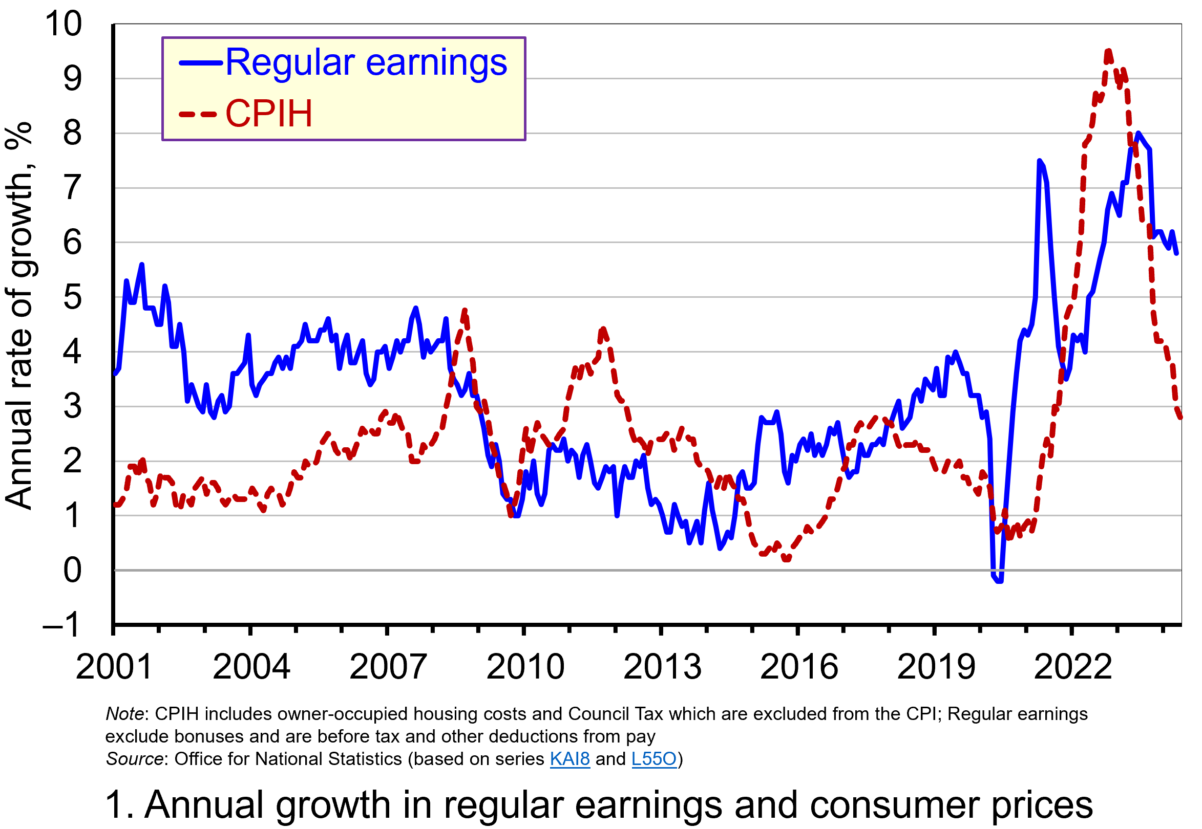 Chart 1 shows the annual percentage changes in actual (nominal) regular weekly pay and the CPIH since January 2001. Each value is simply the percentage change from 12 months earlier. The period up to June 2008 saw the annual growth of weekly pay outstrip the growth of consumer prices – the blue line in the chart is above the red dashed line. Therefore, the real value of pay rose. However, from June 2008 to August 2014 pay growth consistently fell short of the rate of consumer price inflation – the blue line is below the red dashed line. The result was that average real weekly pay fell. (Click here to download a PowerPoint copy of the chart.)
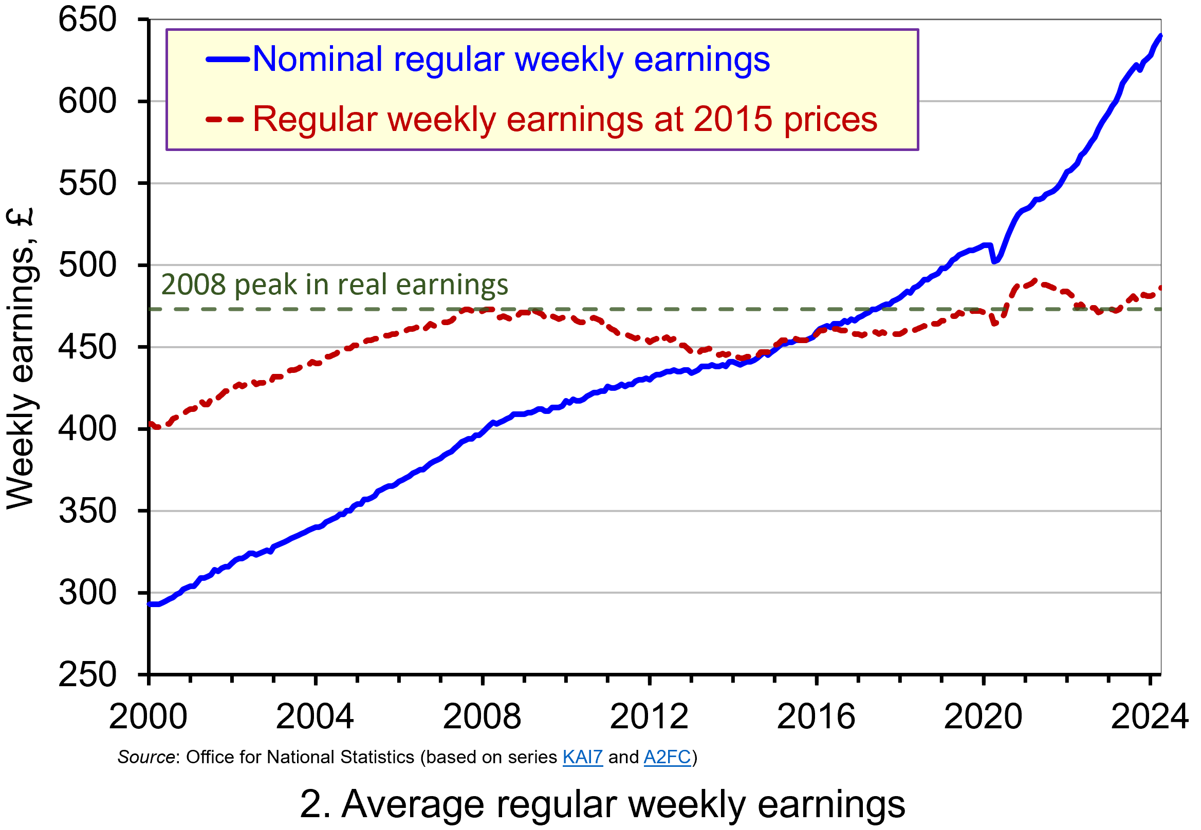 Chart 2 show the average levels of nominal and real weekly pay. The real series is adjusted for inflation. It is calculated by deflating the nominal pay values by the CPIH. Since the CPIH is a price index whose value averages 100 across 2015, the real pay values are at constant 2015 consumer prices. From the chart, we can see that the real value of weekly pay peaked in April 2008 at £473 at 2015 prices. The subsequent period saw rates of pay increases that were lower than rates of consumer price inflation. This meant that by March 2014 the real value of weekly pay had fallen by 6.3 per cent to £443 at 2015 prices. (Click here to download a PowerPoint copy of the chart.)
Although real (inflation-adjusted) pay recovered a little after 2014, 2017 again saw consumer price inflation rates greater than those of pay inflation (see Chart 1). This meant that at the start of 2018 real earnings were 3.2 per cent lower than their 2008-peak (see Chart 2). Real earnings then began to recover, buoyed by the economic rebound following the relaxation of COVID lockdown measures and increasing staffing pressures. Real earnings finally passed their 2008-peak in August 2020. By April 2021 regular weekly pay reached £491 at 2015 prices which was 3.8 per cent above the pre-global financial crisis peak.
However, the boost to real wages was to be short-lived as inflationary pressures rose markedly. While some of this was attributable to the same pressures that were driving up wages, inflationary pressures were fuelled further by the commodity price shock arising from Russia’s invasion of Ukraine and, in particular, its impact on energy prices. This saw the CPIH inflation rate rise to 9.6 per cent in October 2022 (while the CPI inflation rate peaked in the same month at 11.1 per cent). The result was that real weekly earnings fell by 2.7 per cent between January and October 2022 to stand at £471 at 2015 consumer prices. Consequently, average pay was once again below its pre-global financial crisis level.
Although inflationary pressures have recently weakened and real earnings have begun to recover, real regular weekly earnings in April 20024 (£486 at 2015 prices) were a mere 2.7 per cent higher than back in the first half of 2008. This compares to a nominal increase of around 58 per cent over the same period thereby demonstrating the importance of the distinction between nominal and real values in understanding what developments in pay mean for the purchasing power of households.
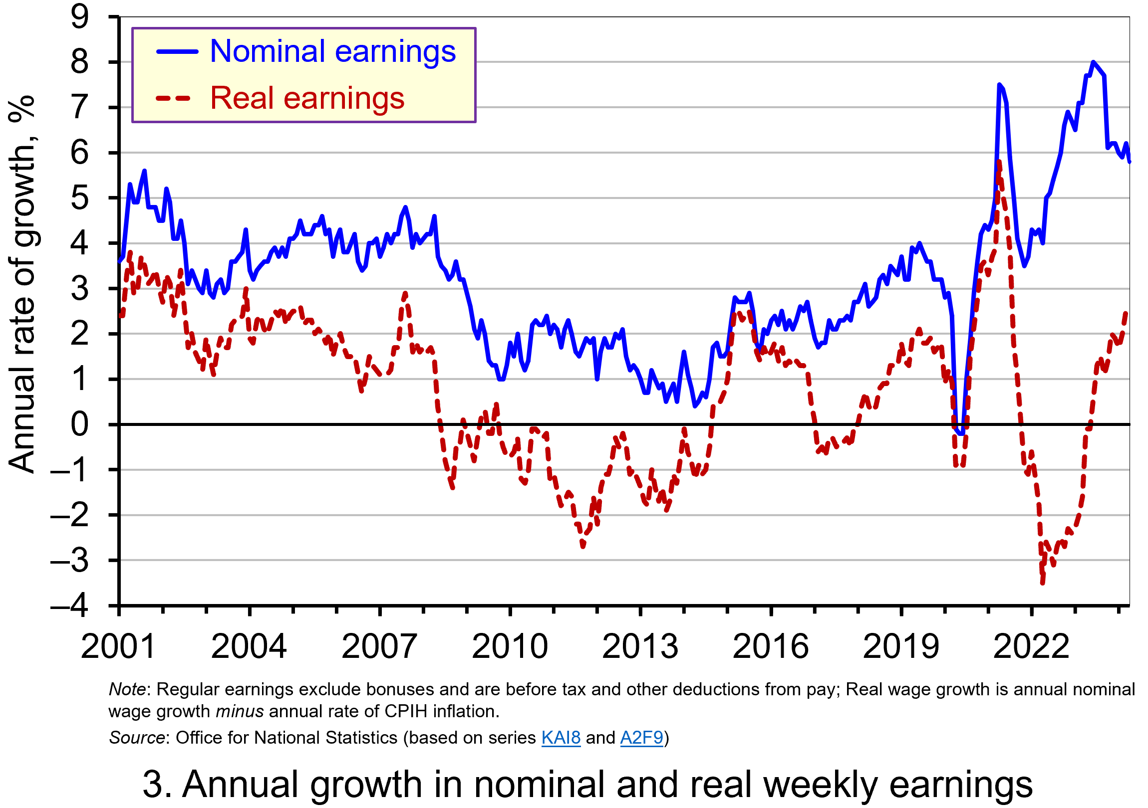 Chart 3 reinforces the importance of the nominal-real distinction. It shows nicely the sustained period of real pay deflation (negative rates of pay inflation) that followed the financial crisis, and the significant rates of real pay deflation associated with the recent inflation shock.
The result is that since June 2008 the average annual rate of growth of real regular weekly pay has been 0.1 per cent, despite nominal pay increasing at an annual rate of 2.9 per cent. In contrast, the period from January 2001 to May 2008 saw real regular weekly pay grow at an annual rate of 2.1 per cent with nominal pay growing at an annual rate of 4.0 per cent. (Click here to download a PowerPoint copy of the chart.)
If we think about the growth of nominal earnings, we can identify two important determinants.
The first is the expected rate of inflation. Workers will understandably want wage growth at least to match the growth in prices so as to maintain their purchasing power.
The second factor is the growth in labour productivity. Firms will be more willing to grant pay increases if workers are more productive, since productivity helps to offset pay increases and maintain firms’ profit margins. Consequently, since over time the actual rate of inflation will tend to mirror the expected rate, the growth of real pay is closely related to the growth of labour productivity. This is significant because, as John discusses in his blog The Productivity Puzzle (14 April 2024), labour productivity growth in the UK, as measured by national output per worker hour, has stalled since the global financial crisis.
Understanding the stagnation of real earnings therefore nicely highlights the interconnectedness of economic variables. In this case, it highlights the connections between productivity, levels of investment and people’s purchasing power. It is not surprising, therefore, that the stagnation of both real earnings and productivity growth since the global financial crisis have become two of the most keenly debated macroeconomic issues of recent times. Indeed, it is likely that their behaviour will continue to shape macroeconomic debates and broader conversations around government policy for some time.
Articles
Questions
- Using the examples of both GDP and earnings, explain how the distinction between nominal and real relates to the distinction between values and volumes.
- In what circumstances would an increase in actual pay translate into a reduction in real pay?
- In what circumstances would a decrease in actual pay translate into an increase in real pay?
- What factors might explain the reduction in real rates of pay seen in the UK following the financial crisis of 2007–8?
- Of what importance might the growth in real rates of pay be for consumption and aggregate demand?
- Why is the growth of real pay an indicator of financial well-being? What other indicators might be included in measuring financial well-being?
- Assume that you have been asked to undertake a distributional analysis of real earnings since the financial crisis. What might be the focus of your analysis? What information would you therefore need to collect?
 Global long-term economic growth has slowed dramatically since the financial crisis of 2007–8. This can be illustrated by comparing the two 20-year periods 1988 to 2007 and 2009 to 2028 (where IMF forecasts are used for 2024 to 2028: see WEO Database under the Data link below). Over the two periods, average annual world growth fell from 3.8% to 3.1%. In advanced countries it fell from 2.9% to 1.6% and in developing countries from 4.8% to 4.3%. In the UK it fell from 2.4% to 1.2%, in the USA from 3.1% to 1.8% and in Japan from 1.9% to 0.5%.
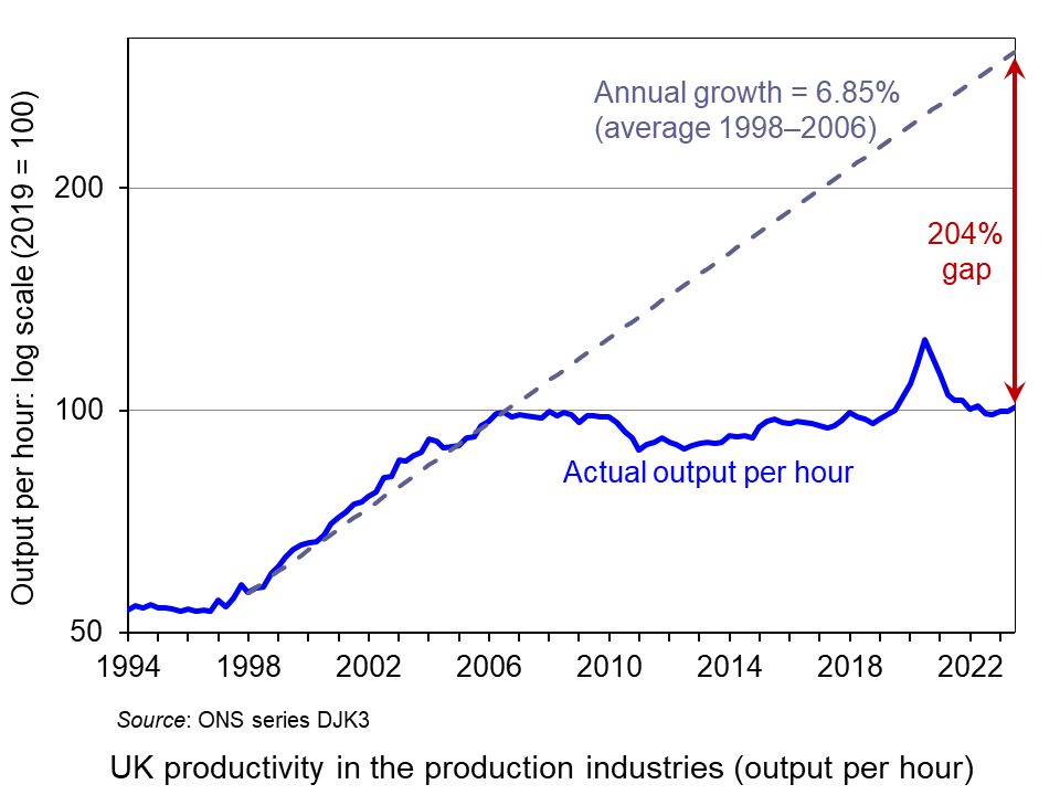 In the UK, labour productivity growth in the production industries was 6.85% per annum from 1998 to 2006. If this growth rate had been maintained, productivity would have been 204% higher by the end of 2023 than it actually was. This is shown in the chart (click here for a PowerPoint).
The key driver of long-term economic growth is labour productivity, which can best be measured by real GDP per hour worked. This depends on three things: the amount of capital per worker, the productivity of this capital and the efficiency of workers themselves – the latter two giving total factor productivity (TFP). Productivity growth has slowed, and with it the long-term rate of economic growth.
If we are measuring growth in output per head of the population, as opposed to simple growth in output, then another important factor is the proportion of the population that works. With ageing populations, many countries are facing an increase in the proportion of people not working. In most countries, these demographic pressures are likely to increase.
 A major determinant of long-term economic growth and productivity is investment. Investment has been badly affected by crises, such as the financial crisis and COVID, and by geopolitical tensions, such as the war in Ukraine and tensions between the USA and China and potential trade wars. It has also been adversely affected by government attempts to deal with rising debt caused by interventions following the financial crisis and COVID. The fiscal squeeze and, more recently higher interest rates, have dampened short-term growth and discouraged investment, thereby dampening long-term growth.
Another factor adversely affecting productivity has been a lower growth of allocative efficiency. Competition in many industries has declined as the rate of new firms entering and exiting markets has slowed. The result has been an increase in concentration and a growth in supernormal profits.
In the UK’s case, growth prospects have also been damaged by Brexit. According to Bank of England and OBR estimates, Brexit has reduced productivity by around 4% (see the blog: The costs of Brexit: a clearer picture). For many companies in the UK, Brexit has hugely increased the administrative burdens of trading with the EU. It has also reduced investment and led to a slower growth in the capital stock.
The UK’s poor productivity growth over many yeas is examined in the blog The UK’s poor productivity record.
Boosting productivity
So, how could productivity be increased and what policies could help the process?
 Artificial intelligence. One important driver of productivity growth is technological advance. The rapid advance in AI and its adoption across much of industry is likely to have a dramatic effect on working practices and output. Estimates by the IMF suggest that some 40% of jobs globally and 60% in advanced countries could be affected – some replaced and others complemented and enhanced by AI. The opportunities for raising incomes are huge, but so too are the dangers of displacing workers and deepening inequality, as some higher-paid jobs are enhanced by AI, while many lower paid jobs are little affected and other jobs disappear.
AI is also likely to increase returns to capital. This may help to drive investment and further boost economic growth. However, the increased returns to capital are also likely to exacerbate inequality.
To guard against the growth of market power and its abuse, competition policies may need strengthening to ensure that the benefits of AI are widely spread and that new entrants are encouraged. Also training and retraining opportunities to allow workers to embrace AI and increase their mobility will need to be provided.
 Training. And it is not just training in the use of AI that is important. Training generally is a key ingredient in encouraging productivity growth. In the UK, there has been a decline in investment in adult education and training, with a 70% reduction since the early 2000s in the number of adults undertaking publicly-funded training, and with average spending on training by employers decreasing by 27% per trainee since 2011. The Institute for Fiscal Studies identifies five main policy levers to address this: “public funding of qualifications and skills programmes, loans to learners, training subsidies, taxation of training and the regulation of training” (see link in articles below).
Competition. Another factor likely to enhance productivity is competition, both internationally and within countries. Removing trade restrictions could boost productivity growth; erecting barriers to protect inefficient domestic industry would reduce it.
Investment. Policies to encourage investment are also key to productivity growth. Private-sector investment can be encouraged by tax incentives. For example, in the UK the Annual Investment Allowance allows businesses to claim 100% of the cost of plant and machinery up to £1m in the year it is incurred. However, for tax relief to produce significant effects on investment, companies need to believe that the policy will stay and not be changed as economic circumstances or governments change.
 Public-sector investment is also key. Good road and rail infrastructure and public transport are vital in encouraging private investment and labour mobility. And investment in health, education and training are a key part in encouraging the development of human capital. Many countries, the UK included, cut back on public-sector capital investment after the financial crisis and this has had a dampening effect on economic growth.
Regional policy. External economies of scale could be encouraged by setting up development areas in various regions. Particular industries could be attracted to specific areas, where local skilled workers, managerial expertise and shared infrastructure can benefit all the firms in the industry. These ‘agglomeration economies’ have been very limited in the UK compared with many other countries with much stronger regional economies.
Changing the aims and governance of firms. A change in corporate structure and governance could also help to drive investment and productivity. According to research by the think tank, Demos (see the B Lab UK article and the second report below), if legislation required companies to consider the social, economic and environmental impact of their business alongside profitability, this could have a dramatic effect on productivity. If businesses were required to be ‘purpose-led’, considering the interests of all their stakeholders, this supply-side reform could dramatically increase growth and well-being.
Such stakeholder-governed businesses currently outperform their peers with higher levels of investment, innovation, product development and output. They also have higher levels of staff engagement and satisfaction.
Articles
- World Must Prioritize Productivity Reforms to Revive Medium-Term Growth
IMF Blog, Nan Li and Diaa Noureldin (10/4/24)
- Why has productivity slowed down?
Oxford Martin School News, Ian Goldin, Pantelis Koutroumpis, François Lafond and Julian Winkler (18/3/24)
- How can the UK revive its ailing productivity?
Economics Observatory, Michelle Kilfoyle (14/3/24)
- With the UK creeping out of recession, here’s an economist’s brief guide to improving productivity
The Conversation, Nigel Driffield (13/3/24)
- UK economy nearly a third smaller thanks to ‘catastrophically bad’ productivity slowdown
City A.M., Chris Dorrell (12/3/24)
- Can AI help solve the UK’s public sector productivity puzzle?
City A.M., Chris Dorrell (11/3/24)
- AI Will Transform the Global Economy. Let’s Make Sure it Benefits Humanity
IMF Blog, Kristalina Georgieva (14/1/24)
- Productivity and Investment: Time to Manage the Project of Renewal
NIESR, Paul Fisher (12/3/24)
- Productivity trends using key national accounts indicators
Eurostat (15/3/24)
- New report says change to company law could add £149bn to the UK economy
B Lab UK (28/11/23)
- Investment in training and skills: Green Budget Chapter 9
Institute for Fiscal Studies, Imran Tahir (12/10/23)
Reports
Data
Questions
- Why has global productivity growth been lower since 2008 than before 2008?
- Why has the UK’s productivity growth been lower than many other advanced economies?
- How does the short-run macroeconomic environment affect long-term growth?
- Find out why Japan’s productivity growth has been so poor compared with other countries.
- What are likely to be the most effective means of increasing productivity growth?
- How may demand management policies affect the supply side of the economy?
- How may the adoption of an ESG framework by companies for setting objectives affect productivity growth?
 It’s two years since Russia invaded Ukraine. Western countries responded by imposing large-scale sanctions. These targeted a range of businesses, banks and other financial institutions, payments systems and Russian exports and imports. Some $1 trillion of Russian assets were frozen. Many Western businesses withdrew from Russia or cut off commercial ties. In addition, oil and gas imports from Russia have been banned by most developed countries and some developing countries, and a price cap of $60 per barrel has been imposed on Russian oil. What is more, sanctions have been progressively tightened over the past two years. For example, on the second anniversary of the invasion, President Biden announced more than 500 new sanctions against individuals and companies involved in military production and supply chains and in financing Russia’s war effort.
The economy in Russia has also been affected by large-scale emigration of skilled workers, the diversion of workers to the armed forces and the diversion of capital and workers to the armaments industry.
So has the economy of Russia been badly affected by sanctions and these other factors? The IMF in its World Economic Forecast of April 2022 predicted that the Russian economy would experience a steep, two-year recession. But, the Russian economy has fared much better than first predicted and the steep recession never materialised.
In this blog we look at Russia’s economic performance. First, we examine why the Russian economy seems stronger today than forecast two years ago. Then we look at its economic weaknesses directly attributable to the war.
Apparent resilience of the Russian economy
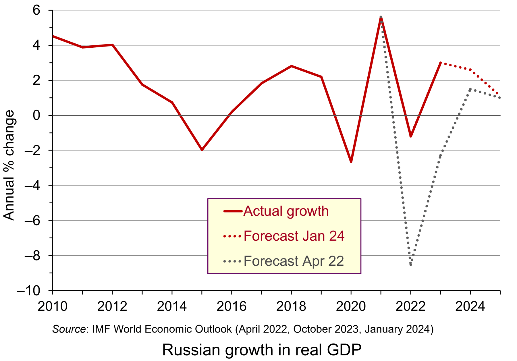 GDP forecasts have proved wrong. In April 2022, just after the start of the war, the IMF was forecasting that the Russian economy would decline by 8.5% in 2022 and by 2.3% in 2023 and grow by just 1.5% in 2024. In practice, the economy declined by only 1.2% in 2022 and grew by 3.0% in 2023. It is forecast by the IMF to grow by 2.6% in 2024. This is illustrated in the chart (click here for a PowerPoint).
Similarly, inflation forecasts have proved wrong. In April 2022, Russian consumer price inflation was forecast to be 21.3% in 2022 and 14.3% in 2023. In practice, inflation was 13.8% in 2022 and 7.4% in 2023. What is more, consumer spending in Russia has remained buoyant. In 2023, retail sales rose by 10.2% in nominal terms – a real rise of 2.8%. Wage growth has been strong and unemployment has remained low, falling from just over 4% in February 2022 to just under 3% today.
So why has the Russian economy seemingly weathered the war so successfully?
 The first reason is that, unlike Ukraine, very little of its infrastructure has been destroyed. Even though it has lost a lot of its military capital, including 1120 main battle tanks and some 2000 other armoured vehicles, virtually all of its production capacity remains intact. What is more, military production is replacing much of the destroyed vehicles and equipment.
The second is that its economy started the war in a strong position economically. In 2021, it had a surplus on the current account of its balance of payments of 6.7% of GDP, reflecting large revenues from oil, gas and mineral exports. This compares with a G7 average deficit of 0.7%. It had fiscal surplus (net general government lending) of 0.8% of GDP. The G7 countries had an average deficit of 9.1% of GDP. Its gross general government debt was 16% of GDP. The G7’s was an average of 134%. This put Russia in a position to finance the war and gave it a considerable buffer against economic sanctions.
 The third reason is that Russia has been effective in switching the destinations of exports and sources of imports. Trade with the West, Japan and South Korea has declined, but trade with China and various neutral countries, such as India have rapidly increased. Take the case of oil: in 2021, Russia exported 4.4 billion barrels of oil per day to the USA, the EU, the UK, Japan and South Korea. By 2023, this had fallen to just 0.6 billion barrels. By contrast, in 2021, it exported 1.9 billion barrels per day to China, India and Turkey. By 2023, this had risen to 4.9 billion. Although exports of natural gas have fallen by around 42% since 2021, Russian oil exports have remained much the same at around 7.4 million barrels per day (until a voluntary cut of 0.5 billion barrels per day in 2024 Q1 as part of an OPEC+ agreement to prop up the price of oil).
China is now a major supplier to Russia of components (some with military uses), commercial vehicles and consumer products (such as cars and electrical goods). Total trade with China (both imports and exports) was worth $147 billion in 2021. By 2023, this had risen to $240 billion.
The use of both the Chinese yuan and the Russian rouble (or ruble) has risen dramatically as a means of payment for Russian imports. Their share has risen from around 5% in 2021 (mainly roubles) to nearly 75% in 2023 (just over 37% in each currency). Switching trade and payment methods has helped Russia to circumvent many of the sanctions.
 The fourth reason is that Russia has a strong and effective central bank. It has successfully used interest rates to control inflation, which is expected to fall from 7.4% in 2023 to under 5% this year and then to its target of 4% in subsequent years. The central bank policy rate was raised from 8.5% to 20% in February 2022. It then fell in steps to 7.5% in September 2022, where it remained until August 2023. It was then raised in steps to peak at 16% in December 2023, where it remains. There is a high level of confidence that the Russian central bank will succeed in bringing inflation back to target.
The fifth reason is that the war has provided a Keynesian stimulus to the economy. Military expenditure has doubled as a share of GDP – from 3.7% of GDP in 2021 to 7.5% in 2024. It now accounts for around 40% of government expenditure. The boost that this has given to production and employment has helped achieve the 3% growth rate in 2023, despite the dampening effect of a tight monetary policy.
Longer-term weaknesses
Despite the apparent resilience of the economy, there are serious weaknesses that are likely to have serious long-term effects.
There has been a huge decline in the labour supply as many skilled and professional workers have move abroad to escape the draft and as many people have been killed in battle. The shortage of workers has led to a rise in wages. This has been accompanied by a decline in labour productivity, which is estimated to have been around 3.6% in 2023.
 Higher wages and lower productivity is putting a squeeze on firms’ profits. This is being exacerbated by higher taxes on firms to help fund the war. Lower profit reduces investment and is likely to have further detrimental effects on labour productivity.
Although Russia has managed to circumvent many of the sanctions, they have still had a significant effect on the supply of goods and components from the West. As sanctions are tightened further, so this is likely to have a direct effect on production and living standards. Although GDP is growing, non-military production is declining.
The public finances at the start of the war, as we saw above, were strong. But the war effort has turned a budget surplus of 0.8% of GDP in 2021 to a deficit of 3.7% in 2023 – a deficit that will be difficult to fund with limited access to foreign finance and with domestic interest rates at 16%. As public expenditure on the military has increased, civilian expenditure has decreased. Benefits and expenditure on infrastructure are being squeezed. For example, public utilities and apartment blocks are deteriorating badly. This has a direct on living standards.
In terms of exports, although by diverting oil exports to China, India and other neutral countries Russia has manage to maintain the volume of its oil exports, revenue from them is declining. Oil prices have fallen from a peak of $125 per barrel in June 2022 to around $80 today. Production from the Arabian Gulf is likely to increase over the coming months, which will further depress oil prices.
Conclusions
With the war sustaining the Russian economy, it would be a problem for Russia if the war ended. If Russia won by taking more territory in Ukraine and forcing Ukraine to accept Russia’s terms for peace, the cost to Russia of rebuilding the occupied territories would be huge. If Russia lost territory and negotiated a settlement on Ukraine’s terms, the political cost would be huge, with a disillusioned Russian people facing reduced living standards that could lead to the overthrow of Putin. As The Conversation article linked below states:
A protracted stalemate might be the only solution for Russia to avoid total economic collapse. Having transformed the little industry it had to focus on the war effort, and with a labour shortage problem worsened by hundreds of thousands of war casualties and a massive brain drain, the country would struggle to find a new direction.
Articles
- How Russia’s economy survived two years of war
The Bell (23/2/24)
- How Russia uses China to get round sanctions
The Bell, Denis Kasyanchuk (20/2/24)
- As Ukraine’s economy burns, Russia clings to a semblance of prosperity
The Observer, Larry Elliott and Phillip Inman (24/2/24)
- ‘A lot higher than we expected’: Russian arms production worries Europe’s war planners
The Guardian, Andrew Roth (15/2/24)
- There are lessons from Russia’s GDP growth — but not the ones Putin thinks
Financial Times, Martin Sandbu (11/2/24)
 Russia’s economy going strong
DW, Miltiades Schmidt (21/2/24)
- The West tried to crush Russia’s economy. Why hasn’t it worked?
Politico, Nahal Toosi, Ari Hawkins, Koen Verhelst, Gabriel Gavin and Kyle Duggan (24/2/24)
- Don’t Buy Putin’s Bluff. The West Can Outspend Him.
Bloomberg UK, Editorial (23/2/24)
- Russia’s war economy cannot last but has bought time
BBC News, Faisal Islam (11/2/24)
- US targets Russia with more than 500 new sanctions
BBC News, George Wright and Will Vernon (24/2/24)
- Russia’s economy is now completely driven by the war in Ukraine – it cannot afford to lose, but nor can it afford to win
The Conversation, Renaud Foucart (22/2/24)
Questions
- Argue the case for and against including military production in GDP.
- How successful has the freezing of Russian assets been?
- How could Western sanctions against Russia be made more effective?
- What are the dangers to Western economies of further tightening financial sanctions against Russia?
- Would it be a desirable policy for a Western economy to divert large amounts of resources to building public infrastructure?
- Has the Ukraine war hastened the rise of the Chinese yuan as a reserve currency?
- How would you summarise Russia’s current public finances?
- How would you set about estimating the cost to Russia of its war with Ukraine?
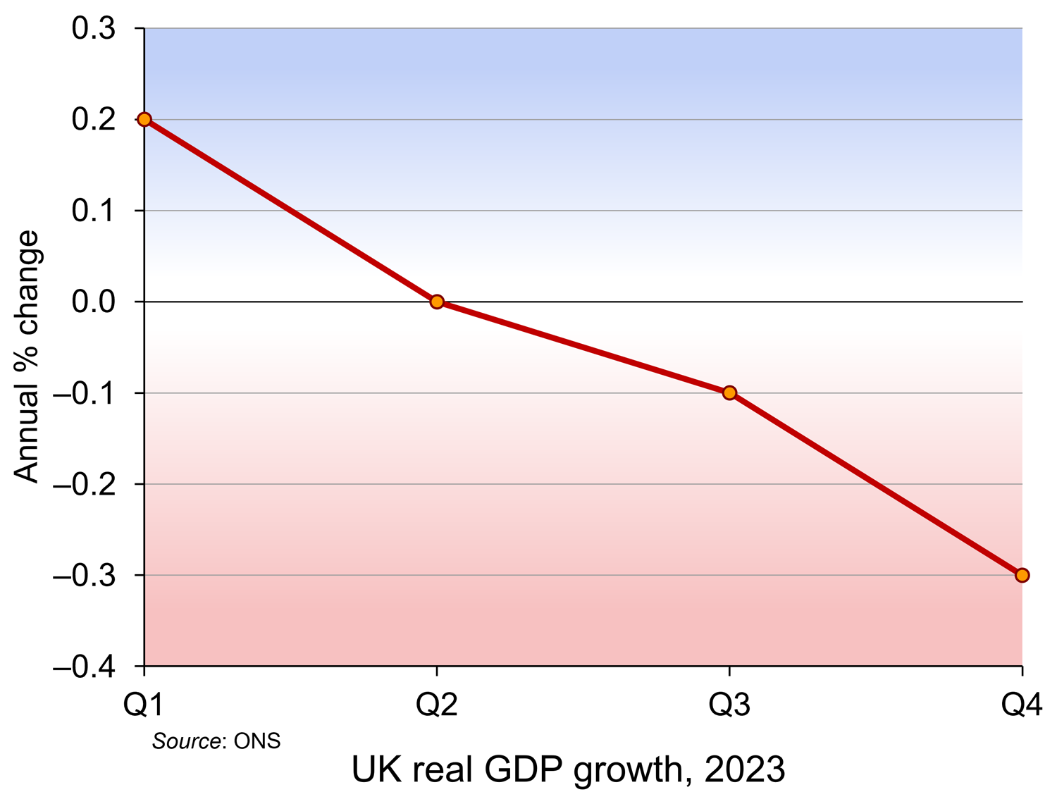 Latest figures from the Office for National Statistics show that the UK was in recession at the end of 2023. The normal definition of recession is two quarters of falling real GDP. This is what happened to the UK in the last two quarters of 2023, with GDP falling by 0.1% in Q3 and 0.3% in Q4. In Q4, output of the service industries fell by 0.2%, production industries by 1.0% and construction by 1.3%.
But how bad is this? What are the implications for living standards? In some respects, the news is not as bad as the term ‘recession’ might suggest. In other respects, it’s worse than the headline figures might imply.
The good news (or not such bad news)
The first thing to note is that other countries too experienced a recession or slowdown in the second half of 2023. So, relative to these countries, the UK is not performing that badly. Japan, for example, also experienced a mild recession; Germany just missed one. These poor economic growth rates were caused largely by higher global energy and food prices and by higher central bank interest rates in response. The good news is that such cost pressures are already easing.
The second piece of good news is that GDP is expected to start growing again (modestly) in 2024. This will be helped by the Bank of England cutting interest rates. The Monetary Policy Committee is expected to do this at its May, June or August meetings provided that inflation falls. Annual CPI inflation was 4% in January – the same as in December. But it is expected to fall quite rapidly over the coming months provided that there are no serious supply-side shocks (e.g. from world political factors).
The third is that the recession is relatively modest compared with ones in the past. In the recession following the financial crisis, real GDP fell by 5.3% in 2009; during the pandemic, GDP fell by 10.7% in 2020. For this reason, some commentators have said that the last two quarters of 2023 represent a mere ‘technical recession’, with the economy expected to grow again in 2024.
Why things may be worse than the headline figures suggest
Real GDP per head
So far we have considered real GDP (i.e. GDP adjusted for inflation). But if changes in GDP are to reflect changes in living standards, we need to consider real GDP per head. Population is rising. This means that the rate of growth in real GDP per head is lower than the rate of growth in real GDP
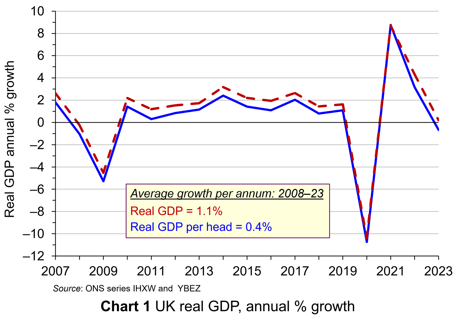 For 2023 as a whole, while real GDP rose by 0.20%, real GDP per head fell by 0.67%. In the last two quarters of 2023, while real GDP fell by 0.1% and 0.3% respectively, real GDP per head fell by 0.4% and 0.6%, respectively, having already fallen in each of the previous five quarters. Chart 1 shows real GDP growth and real GDP growth per head from 2007 to 2023 (click here for a PowerPoint). As you can see, given population growth, real GDP per head has consistently grown slower than real GDP.
Long-term trends.
If we are assessing the UK’s potential for growth in GDP, rather than the immediate past, it is useful to look at GDP growth over a longer period. Looking at past trend growth rates and explaining them can give us an indication of the likely future path of the growth in GDP – at least in the absence of a significant change in underlying economic factors. Since 2007, the average annual rate of growth of real GDP has been only 1.1% and that of real GDP per head a mere 0.4%.
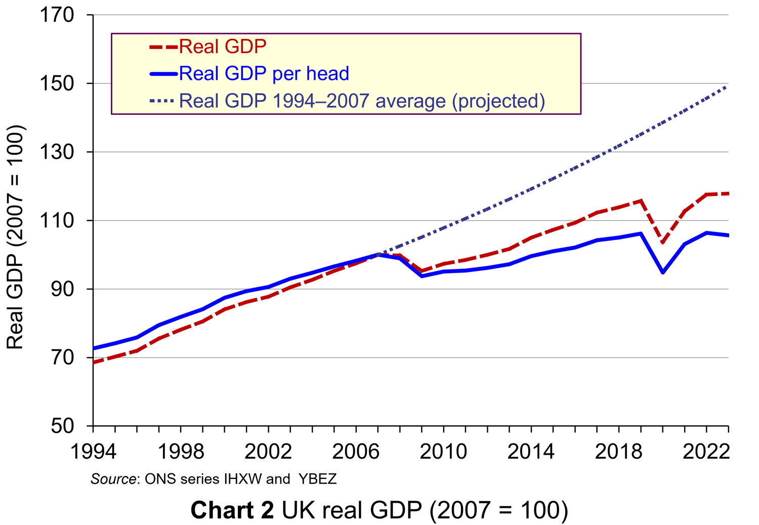 This compares unfavourably with the period from 1994 to 2007, when the average annual rate of growth of real GDP was 3.0% and that of real GDP per head was 2.5%.
This is illustrated in Chart 2 (click here for a PowerPoint). The chart also projects the growth rate in GDP per head of 2.5% forward from 2007 to 2023. Had this growth rate been achieved since 2007, GDP per head in 2023 would have been 41.4% higher than it actually was.
It is not only the UK that has seen low growth over the past 15 years compared to previous years. It has achieved a similar average annual growth rate over the period to Germany (1.1%), lower rates than the USA (1.8%) and Canada (1.6%), but higher than France (0.9%) and Japan (0.4%).
Low investment
A key determinant of economic growth is investment. Since 2008, the UK has invested an average of 17.3% of GDP. This is the lowest of the G7 countries and compares with 24.9% in Japan, 23.7% in Canada, 23.5% in France, 21.3% in Germany, 20.4% in the USA and 19.1% in Italy. If UK growth is to recover strongly over the longer term, the rate of investment needs to increase, both private and public. Of course, investment has to be productive, as the key underlying determinant of economic growth is the growth in productivity.
Low productivity growth
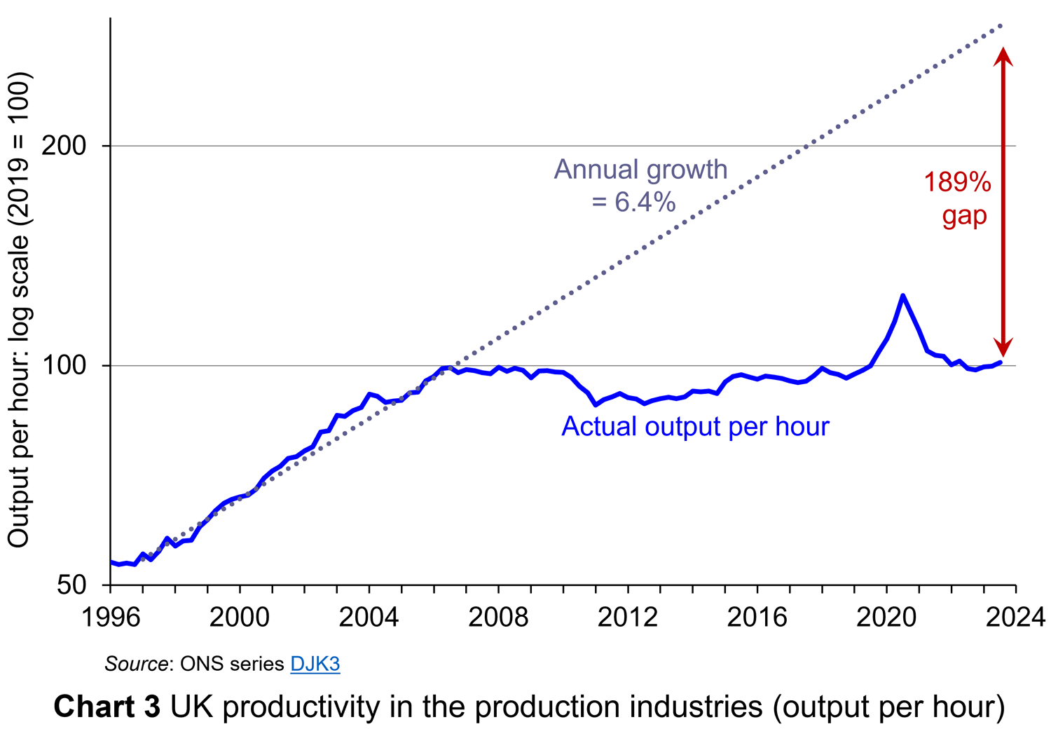 This is a key issue for the government – how to encourage a growth in productivity. The UK’s record of productivity growth has been poor since 2008. The period from 1996 to 2006 saw an average annual growth in labour productivity of 6.4%. Since then, however, labour productivity has grown by an average annual rate of only 0.3%. This is illustrated in Chart 3 (click here for a PowerPoint). If the pre-2007 rate had continued to the end of 2023, labour productivity would be 189% higher. This would have made GDP per head today substantially higher. If GDP per head is to grow faster, then the underlying issue of a poor growth in labour productivity will need to be addressed.
Inequality and poverty
Then there is the issue of the distribution of national income. The UK has a high level of income inequality. In 2022 (the latest data available), the disposable income of the poorest 20% of households was £13 218; that for the richest 20% was £83 687.  The top 1% of income earners’ share of disposable income is just under 9.0%. (Note that disposable income is after income taxes have been deducted and includes cash benefits and is thus more equally distributed than original income.)
The poorest 20% have been hit badly by the cost-of-living crisis, with many having to turn to food banks and not being able to afford to heat their homes adequately. They are also particularly badly affected by the housing crisis, with soaring and increasingly unaffordable rents. Many are facing eviction and others live in poor quality accommodation. Simple growth rates in real GDP do not capture such issues.
Limited scope for growth policies
Fiscal policy has an important role in stimulating growth. Conservatives stress tax cuts as a means of incentivising entrepreneurs and workers. Labour stresses the importance of public investment in infrastructure, health, education and training. Either way, such stimulus policy requires financing.
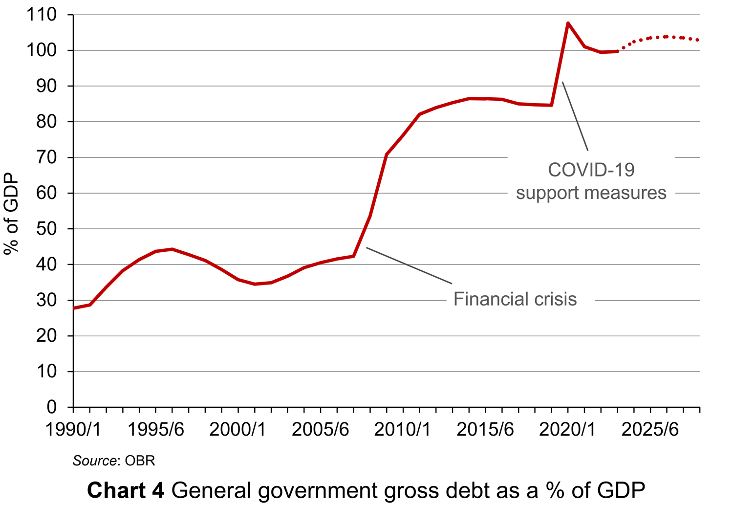 But, public finances have been under pressure in recent years, especially from COVID support measures. General government gross debt has risen from 27.7% of GDP in 1990/91 to 99.4% in 2022/23. This is illustrated in Chart 4 (click here for a PowerPoint). Although it has fallen from the peak of 107.6% of GDP in 2020/21 (during the COVID pandemic), according to the Office for Budget Responsibility it is set to rise again, peaking at 103.8% in 2026/27. There is thus pressure on the government to reduce public-sector borrowing, not increase it. This makes it difficult to finance public investment or tax cuts.
Measuring living standards
Questions about real GDP have huge political significance. Is the economy in recession? What will happen to growth in GDP over the coming months. Why has growth been sluggish in recent years? The implication is that if GDP rises, living standards will rise; if GDP falls, living standards will fall. But changes in GDP, even if expressed in terms of real GDP and even if the distribution of GDP is taken into account, are only a proxy for living standards. GDP measures the market value of the output of goods and services and, as such, may not necessarily be a good indicator of living standards, let alone well-being.
Produced goods and services that are not part of GDP
 The output of some goods and services goes unrecorded. As we note in Economics, 11e (section 15.2), “If you employ a decorator to paint your living room, this will be recorded in the GDP statistics. If, however, you paint the room yourself, it will not. Similarly, if a childminder is employed by parents to look after their children, this childcare will form part of GDP. If, however, a parent stays at home to look after the children, it will not.
The exclusion of these ‘do-it-yourself’ and other home-based activities means that the GDP statistics understate the true level of production in the economy. If over time there is an increase in the amount of do-it-yourself activities that people perform, the figures will also understate the rate of growth of national output.” With many people struggling with the cost of living, such a scenario is quite likely.
There are also activities that go unrecorded in the ‘underground’ or ‘shadow’ economy: unemployed people doing casual jobs for cash in hand that they do not declare to avoid losing benefits; people doing extra work outside their normal job and not declaring the income to evade taxes; builders doing work for cash to save the customer paying VAT.
Externalities
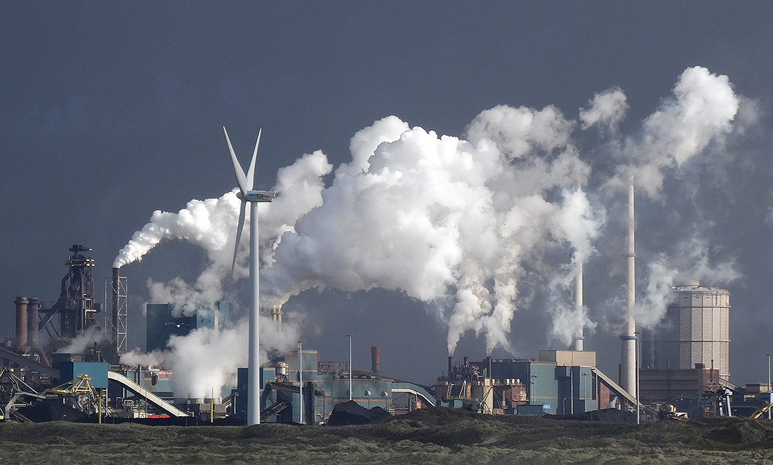 Large amounts of production and consumption involve external costs to the environment and to other people. These externalities are not included in the calculation of GDP.
If external costs increase faster than GDP, then GDP growth will overstate the rise in living standards. If external costs rise more slowly than GDP (or even fall), then GDP growth will understate the rise in living standards. We assume here that living standards include social and environmental benefits and are reduced by social and environmental costs.
Human costs of production
If production increases as a result of people having to work harder or longer hours, its net benefit will be less. Leisure is a desirable good, and so too are pleasant working conditions, but these items are not included in the GDP figures.
The production of certain ‘bads’ leads to an increase in GDP
 Some of the undesirable effects of growth may in fact increase GDP! Take the examples of crime, stress-related illness and environmental damage. Faster growth may lead to more of all three. But increased crime leads to more expenditure on security; increased stress leads to more expenditure on health care; and increased environmental damage leads to more expenditure on environmental clean-up. These expenditures add to GDP. Thus, rather than reducing GDP, crime, stress and environmental damage actually increase it.
Alternative approaches to measuring production and income
There have been various attempts to adjust GDP (actual or potential) to make it a better indicator of total production or income or, more generally, of living standards.
Index of Sustainable Economic Welfare (ISEW)
As Case Study 9.20 in the Essentials of Economics (9e) website explains, ISEW starts with consumption, as measured in GDP, and then makes various adjustments to account for factors that GDP ignores. These include:
- Inequality: the greater the inequality, the more the figure for consumption is reduced. This is based on the assumption of a diminishing marginal utility of income, such that an additional pound is worth less to a rich person than to a poor person.
- Household production (such as childcare, care for the elderly or infirm, housework and various do-it-yourself activities). These ‘services of household labour’ add to welfare and are thus entered as a positive figure.
- Defensive expenditures. This is spending to offset the adverse environmental effects of economic growth (e.g. asthma treatment for sufferers whose condition arises from air pollution). Such expenditures are taken out of the calculations.
- ‘Bads’ (such as commuting costs). The monetary expense entailed is entered as a negative figure (to cancel out its measurement in GDP as a positive figure) and then an additional negative element is included for the stress incurred.
- Environmental costs. Pollution is entered as a negative figure.
- Resource depletion and damage. This too is given a negative figure, in just the same way that depreciation of capital is given a negative figure when working out net national income.
Productive Capacities Index (PCI)
In 2023, the United Nations Conference on Trade and Development (UNCTAD) launched a new index to provide a better measure of countries’ economic potential. What the index focuses on is not actual GDP but potential output: in other words, ‘countries’ abilities to produce goods and deliver services’.
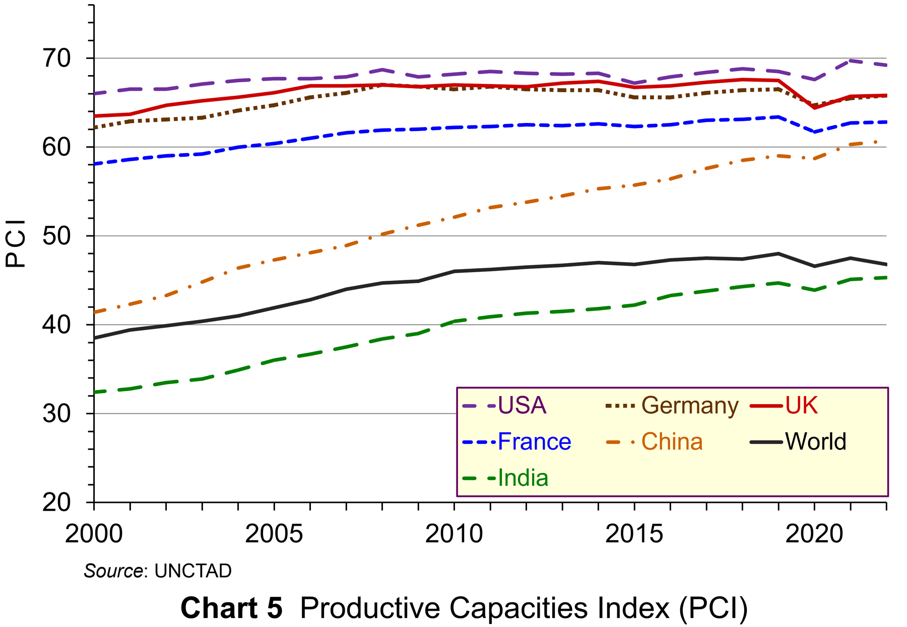 The PCI comprises 42 indicators under eight headings: human capital, natural capital, information and communication technology (ICT), structural change (the movement of labour and other productive resources from low-productivity to high-productivity economic activities), transport infrastructure, institutions (political, legal and financial) and the private sector (ease of starting businesses, availability of credit, ease of cross-border trade, etc.). It covers 194 economies since 2000 (currently to 2022). As UNCTAD states, ‘The PCI can help diagnose the areas where countries may be leading or falling behind, spotlighting where policies are working and where corrective efforts are needed.’ Chart 5 shows the PCI for various economies from 2000 to 2022 (click here for a PowerPoint).
The UK, with a PCI of 65.8 in 2022, compares relatively favourably with other developed countries. The USA’s PCI is somewhat higher (69.2), as is The Netherlands’ (69.8); Germany’s is the same (65.8); France’s is somewhat lower (62.8). The world average is 46.8. For developing countries, China is relatively high (60.7); India’s (45.3) is close to the developing country average of 43.4.
Looked at over a longer time period, the UK’s performance is relatively weak. The PCI in 2022 (65.8) was below that in 2006 (66.9) and below the peak of 67.6 in 2018.
GDP and well-being
GDP is often used as a proxy for well-being. If real GDP per head increases, then it is assumed that well-being will increase. In practice, people’s well-being depends on many factors, not just their income, although income is one important element.
The UK Measuring National Well-being (MNW) programme
 The MNW programme was established in 2010. This has resulted in Office for National Statistics developing new measures of national well-being. The ONS produces statistical bulletins and datasets with its latest results.
The aim of the programme is to provide a ‘fuller picture’ of how society is doing beyond traditional economic indicators. There are currently 44 indicators. These are designed to describe ‘how we are doing as individuals, as communities and as a nation, and how sustainable this is for the future’. The measures fall within a number of categories, including: personal well-being, relationships, health, what we do, where we live, personal finance, the economy, education and skills, governance and the natural environment.
Conclusions
In the light of the limitations of GDP as a measure of living standards, what can we make of the news that the UK entered recession in the last half of 2023? It does show that the economy is sluggish and that the production of goods and services that are included in the GDP measure declined.
But to get a fuller assessment of the economy, it is important to take a number of other factors into account. If we are to go further and ask what has happened to living standards or to well-being, then we have to look at a range of other factors. If we are to ask what the latest figures tell us about what is likely to happen in the future to production, living standards and well-being, then we will need to look further still.
Articles
- Britain falls into recession, with worst GDP performance in 2023 in years
CNN, Hanna Ziady (15/2/24)
- UK economy slipped into recession in 2023
Financial Times, Valentina Romei and George Parker (15/2/24)
- UK economy fell into recession after people cut spending
BBC News, Dearbail Jordan & Faisal Islam (15/2/24)
- Should we care that the UK is in recession?
BBC News, Faisal Islam (15/2/24)
- UK tips into recession in blow to Rishi Sunak
The Guardian, Richard Partington (15/2/24)
- Britain is in recession… and huge immigration has been masking how much poorer we’re getting
MSN, James Tapsfield (15/2/24)
- This isn’t a “mild” recession
The New Statesman, Duncan Weldon (15/2/24)
- UK middle classes ‘struggling despite incomes of up to £60,000 a year’
The Guardian, Larry Elliott (20/2/24)
- What is GDP and how is it measured?
BBC News (15/2/24)
 World at One (from 7’00” to 25’14”)
BBC Sounds, Torsten Bell and Norman Lamont (15/2/24)
- Does High GDP Mean Economic Prosperity?
Investopedia, Lisa Smith (29/9/23)
- A critical assessment of GDP as a measure of economic performance and social progress
Carnegie UK, Cressida Gaukroger (June 2023)
- When it comes to measuring economic welfare, GDP doesn’t cut it
Marketplace, Kai Ryssdal and Maria Hollenhorst (1/9/23)
- UNCTAD launches new index for countries to better measure economic potential
UNCTAD News (20/6/23)
- Redefining Economic Growth for a Climate-Conscious World
Forbes, Judah Taub (28/9/23)
- Bobby Kennedy on GDP: ‘measures everything except that which is worthwhile’
The Guardian, Simon Rogers (24/5/12)
- A guide to the UK National Accounts: Satellite Accounts
ONS (6/3/20)
Data and Analysis
- GDP first quarterly estimate, UK: October to December 2023
ONS (15/2/24)
- GDP (Average) per head, q-on-q4 growth rate CVM SA % (series N3Y8)
ONS
- Gross domestic product (Average) per head, CVM market prices: SA (series IHXW)
ONS
- GDP per capita, current prices (UK)
IMF
- Productive capacities index, annual, 2000-2022
UNCTAD
- The Scale of Economic Inequality in the UK
The Equality Trust (2023)
- Living standards, poverty and inequality in the UK: 2023
IFS, Sam Ray-Chaudhuri, Tom Waters, Thomas Wernham and Xiaowei Xu (July 2023)
- Quarterly personal well-being estimates – seasonally adjusted
ONS
Questions
- Using GDP and other data, summarise the outlook for the UK economy.
- Why is GDP so widely used as an indicator of living standards?
- Explain the three methods of measuring GDP?
- What key contributors to living standards are omitted from GDP?
- What are the ONS Satellite Accounts? Are they useful for measuring living standards?
- Assess the UK’s economic potential against each of the eight category indices in the Productive Capacities Index.
- What is the difference between ‘living standards’ and ‘well-being’?
 According to the IMF, Chinese GDP grew by 5.2% in 2023 and is predicted to grow by 4.6% this year. Such growth rates would be extremely welcome to most developed countries. UK growth in 2023 was a mere 0.5% and is forecast to be only 0.6% in 2024. Advanced economies as a whole only grew by 1.6% in 2023 and are forecast to grow by only 1.5% this year. Also, with the exception of India, the Philippines and Indonesia, which grew by 6.7%, 5.3% and 5.0% respectively in 2023 and are forecast to grow by 6.5%, 6.0% and 5.0% this year, Chinese growth also compares very favourably with other developing countries, which as a weighted average grew by 4.1% last year and are forecast to grow at the same rate this year.
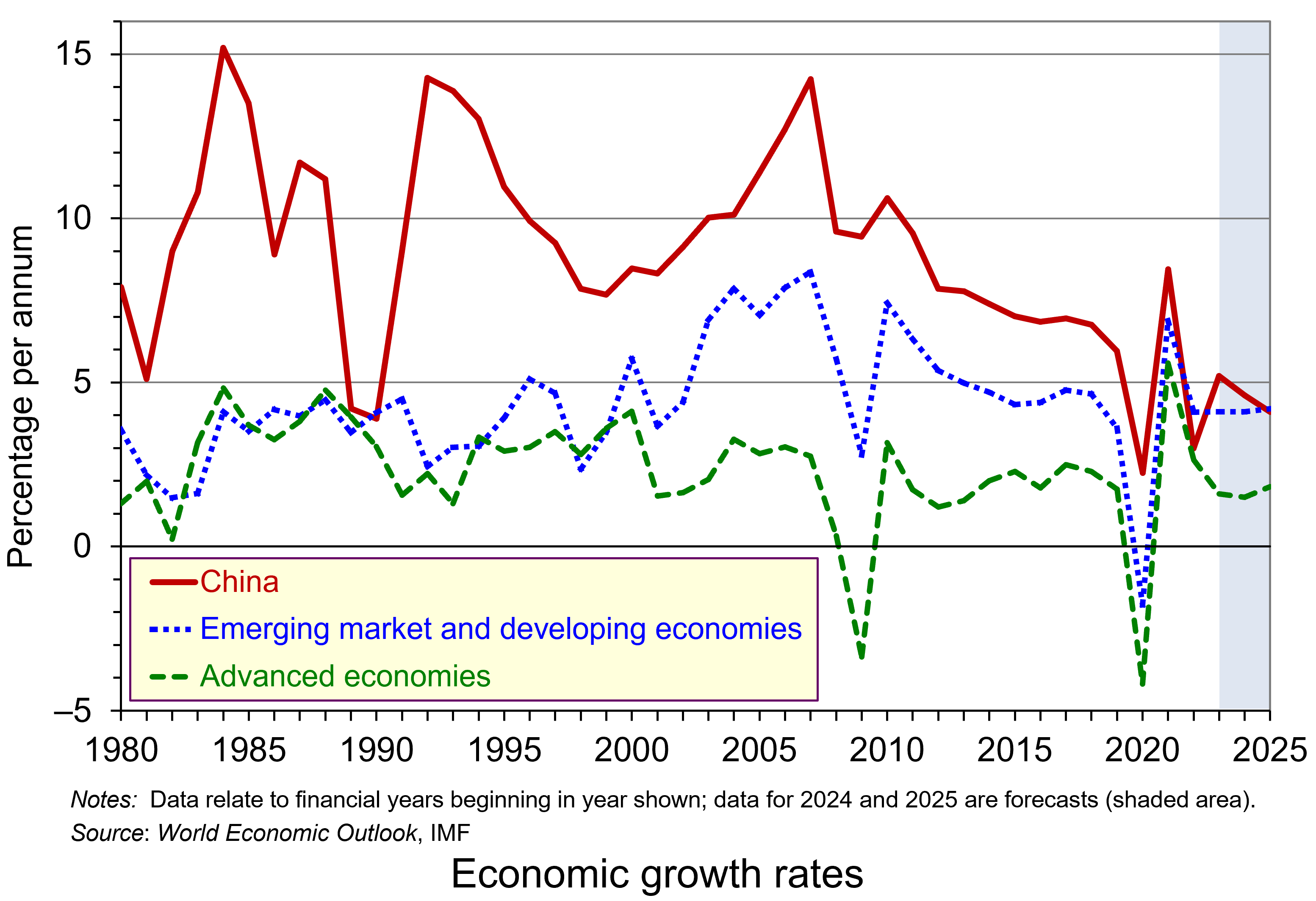 But in the past, Chinese growth was much higher and was a major driver of global growth. Over the period 1980 to 2018, Chinese economic growth averaged 9.5% – more than twice the average rate of developing countries (4.5%) and nearly four times the average rate of advanced countries (2.4%) (see chart – click here for a PowerPoint of the chart).
Not only is Chinese growth now much lower, but it is set to decline further. The IMF forecasts that in 2025, Chinese growth will have fallen to 4.1% – below the forecast developing-country average of 4.2% and well below that of India (6.5%).
Causes of slowing Chinese growth
There are a number of factors that have come together to contribute to falling economic growth rates – growth rates that otherwise would have been expected to be considerably higher as the Chinese economy reopened after severe Covid lockdowns.
 Property market
China has experienced a property boom over the past 20 years years as the government has encouraged construction in residential blocks and in factories and offices. The sector has accounted for some 20% of economic activity. But for many years, demand outstripped supply as consumers chose to invest in property, partly because of a lack of attractive alternatives for their considerable savings and partly because property prices were expected to go on rising. This lead to speculation on the part of both buyers and property developers. Consumers rushed to buy property before prices rose further and property developers borrowed considerably to buy land, which local authorities encouraged, as it provided a valuable source of revenue.
But now there is considerable overcapacity in the sector and new building has declined over the past three years. According to the IMF:
Housing starts have fallen by more than 60 per cent relative to pre-pandemic levels, a historically rapid pace only seen in the largest housing busts in cross-country experience in the last three decades. Sales have fallen amid homebuyer concerns that developers lack sufficient financing to complete projects and that prices will decline in the future.
As a result, many property developers have become unviable. At the end of January, the Chinese property giant, Evergrande, was ordered to liquidate by a Hong Kong court, after the judge ruled that the company did not have a workable plan to restructure around $300bn of debt. Over 50 Chinese property developers have defaulted or missed payments since 2020. The liquidation of Evergrande and worries about the viability of other Chinese property developers is likely to send shockwaves around the Chinese property market and more widely around Chinese investment markets.
Overcapacity
Rapid investment over many years has led to a large rise in industrial capacity. This has outstripped demand. The problem could get worse as investment, including state investment, is diverted from the property sector to manufacturing, especially electric vehicles. But with domestic demand dampened, this could lead to increased dumping on international markets – something that could spark trade wars with the USA and other trading partners (see below). Worries about this in China are increasing as the possibility of a second Trump presidency looks more possible. The Chinese authorities are keen to expand aggregate demand to tackle this overcapacity.
Uncertainty
Consumer and investor confidence are low. This is leading to severe deflationary pressures. If consumers face a decline in the value of their property, this wealth effect could further constrain their spending. This will, in turn, dampen industrial investment.
Uncertainty is beginning to affect foreign companies based in China. Many foreign companies are now making a loss in China or are at best breaking even. This could lead to disinvestment and add to deflationary pressures.
The Chinese stock market and policy responses
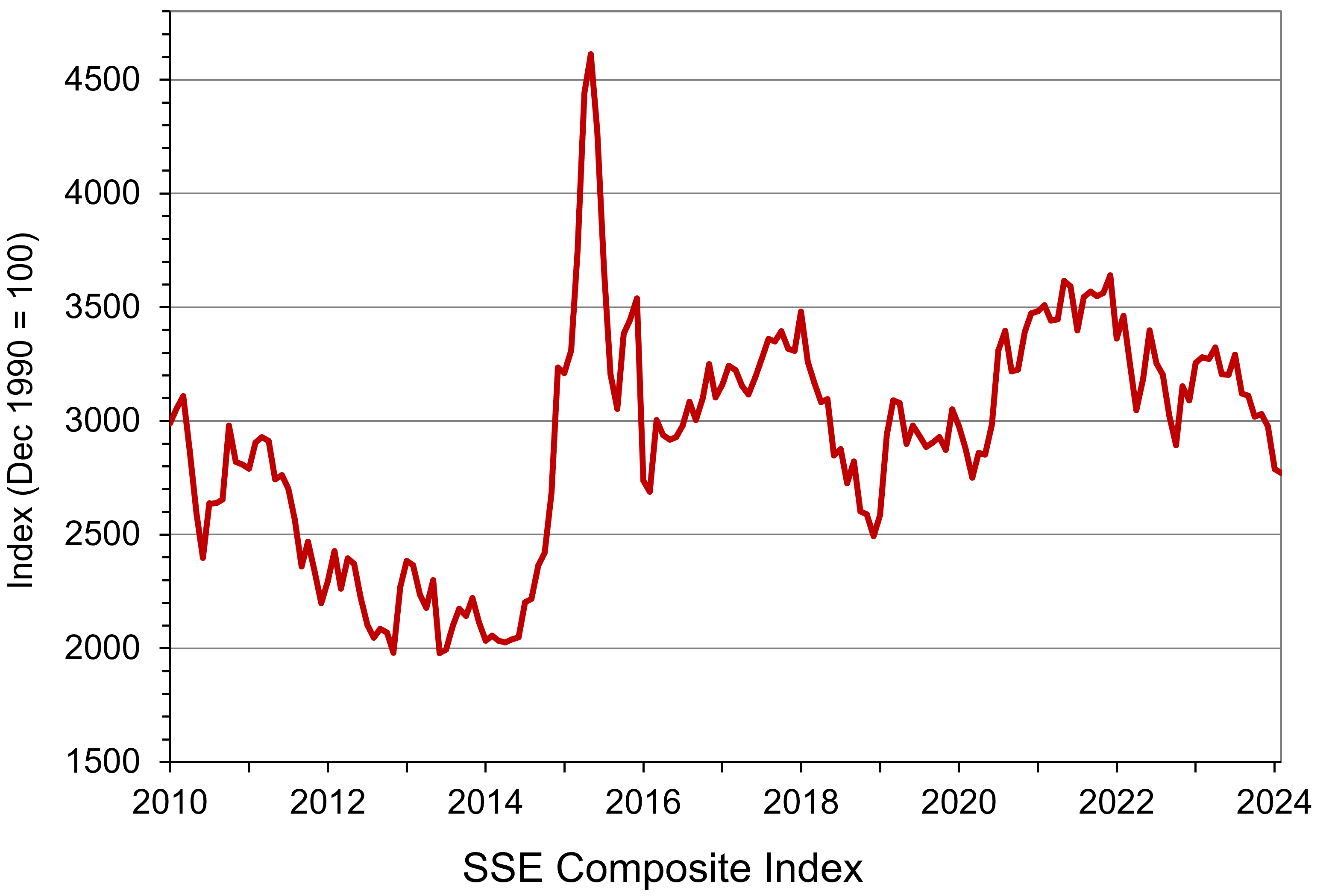 Lack of confidence in the Chinese economy is reflected in falling share prices. The Shanghai SSE Composite Index (an index of all stocks traded on the Shanghai Stock Exchange) has fallen dramatically in recent months. From a high of 3703 in September 2021, it had fallen to 2702 on 5 Feb 2024 – a fall of 27%. It is now below the level at the beginning of 2010 (see chart: click here for a PowerPoint). On 5 February alone, some 1800 stocks fell by over 10% in Shanghai and Shenzhen. People were sensing a rout and investors expressed their frustration and anger on social media, including the social media account of the US Embassy. The next day, the authorities intervened and bought large quantities of key stocks. China’s sovereign wealth fund announced that it would increase its purchase of shares to support the country’s stock markets. The SSE Composite rose 4.1% on 6 February and the Shenzhen Component Index rose 6.2%.
However, the rally eased as investors waited to see what more fundamental measures the authorities would take to support the stock markets and the economy more generally. Policies are needed to boost the wider economy and encourage a growth in consumer and business confidence.
Interest rates have been cut four times since the beginning of 2022, when the prime loan rate was cut from 3.85% to 3.7%. The last cut was from 3.55% to 3.45% in August 2023. But this has been insufficient to provide the necessary boost to aggregate demand. Further cuts in interest rates are possible and the government has said that it will use proactive fiscal and effective monetary policy in response to the languishing economy. However, government debt is already high, which limits the room for expansionary fiscal policy, and consumers are highly risk averse and have a high propensity to save.
Graduate unemployment
 China has seen investment in education as an important means of increasing human capital and growth. But with a slowing economy, there are are more young people graduating each year than there are graduate jobs available. Official data show that for the group aged 16–24, the unemployment rate was 14.9% in December. This compares with an overall urban unemployment rate of 5.1%. Many graduates are forced to take non-graduate jobs and graduate jobs are being offered at reduced salaries. This will have a further dampening effect on aggregate demand.
Demographics
China’s one-child policy, which it pursued from 1980 to 2016, plus improved health and social care leading to greater longevity, has led to an ageing population and a shrinking workforce. This is despite recent increases in unemployment in the 16–24 age group. The greater the ratio of dependants to workers, the greater the brake on growth as taxes and savings are increasingly used to provide various forms of support.
Effects on the rest of the world
China has been a major driver of world economic growth. With a slowing Chinese economy, this will provide less stimulus to growth in other countries. Many multinational companies, including chip makers, cosmetics companies and chemical companies, earn considerable revenue from China. For example, the USA exports over $190 billion of goods and services to China and these support over 1 million jobs in the USA. A slowdown in China will have repercussions for many companies around the world.
There is also the concern that Chinese manufacturers may dump products on world markets at less than average (total) cost to shift stock and keep production up. This could undermine industry in many countries and could initiate a protectionist response. Already Donald Trump is talking about imposing a 10% tariff on most imported goods if he is elected again in November. Such tariffs could be considerably higher on imports from China. If Joe Biden is re-elected, he too may impose tariffs on Chinese goods if they are thought to be unfairly subsidised. US (and possibly EU) tariffs on Chinese goods could lead to a similar response from China, resulting in a trade war – a negative sum game.
Videos
Articles
- IMF Predicts China Economy Slowing Over Next Four Years
Voice of America, Evie Steele (2/2/24)
- China’s Real Estate Sector: Managing the Medium-Term Slowdown
IMF News, Henry Hoyle and Sonali Jain-Chandra (2/2/24)
- China braced for largest human migration on earth amid bleak economic backdrop
ITV News, Debi Edward (4/2/24)
- China’s property giant Evergrande ordered to liquidate as debt talks fail
Aljazeera (29/1/24)
- China’s overcapacity a challenge that is ‘here to stay’, says US chamber
Financial Times, Joe Leahy (1/2/24)
- China needs to learn lessons from 1990s Japan
Financial Times, Gillian Tett (1/2/24)
- The Trump factor is looming over China’s markets
Financial Times, Katie Martin (2/2/24)
- China’s many systemic problems dominate its outlook for 2024
The Guardian, George Magnus (1/1/24)
- China youth unemployment will stay elevated in 2024, but EIU warns economic impact will linger
CNBC, Clement Tan (25/1/24)
- Don’t count on a soft landing for the world economy – turbulence is ahead
The Guardian, Kenneth Rogoff (2/2/24)
- As falling stocks draw criticism in China, censors struggle to keep up
Washington Post, Lily Kuo (6/2/24)
- China’s doom loop: a dramatically smaller (and older) population could create a devastating global slowdown
The Conversation, Jose Caballero (12/2/24)
- China: why the country’s economy has hit a wall – and what it plans to do about it
The Conversation, Hong Bo (19/3/24)
- Confronting inflation and low growth
OECD Economic Outlook Interim Report (September 2023) (see especially Box 1)
Questions
- Why is China experiencing slowing growth and is growth likely to pick up over the next five years?
- How does the situation in China today compare with that in Japan 30 years ago?
- What policies could the Chinese government pursue to stimulate economic growth?
- What policies were enacted towards China during the Trump presidency from 2017 to 2020?
- Would you advise the Chinese central bank to cut interest rates further? Explain.
- Should China introduce generous child support for families, no matter the number of children?
 In the first of a series of updated blogs focusing on the importance of the distinction between nominal and real values we look at the issue of earnings. Here we update the blog Getting Real with Pay written back in February 2019. Then, we noted how the macroeconomic environment since the financial crisis of the late 2000s had continued to affect people’s pay. Specifically, we observed that there had been no growth in real or inflation-adjusted pay. In other words, people were no better off in 2019 than in 2008.
 Chart 1 shows the annual percentage changes in actual (nominal) regular weekly pay and the CPIH since January 2001. Each value is simply the percentage change from 12 months earlier. The period up to June 2008 saw the annual growth of weekly pay outstrip the growth of consumer prices – the blue line in the chart is above the red dashed line. Therefore, the real value of pay rose. However, from June 2008 to August 2014 pay growth consistently fell short of the rate of consumer price inflation – the blue line is below the red dashed line. The result was that average real weekly pay fell. (Click here to download a PowerPoint copy of the chart.)
 Chart 2 show the average levels of nominal and real weekly pay. The real series is adjusted for inflation. It is calculated by deflating the nominal pay values by the CPIH. Since the CPIH is a price index whose value averages 100 across 2015, the real pay values are at constant 2015 consumer prices. From the chart, we can see that the real value of weekly pay peaked in April 2008 at £473 at 2015 prices. The subsequent period saw rates of pay increases that were lower than rates of consumer price inflation. This meant that by March 2014 the real value of weekly pay had fallen by 6.3 per cent to £443 at 2015 prices. (Click here to download a PowerPoint copy of the chart.)
 Chart 3 reinforces the importance of the nominal-real distinction. It shows nicely the sustained period of real pay deflation (negative rates of pay inflation) that followed the financial crisis, and the significant rates of real pay deflation associated with the recent inflation shock.
 Global long-term economic growth has slowed dramatically since the financial crisis of 2007–8. This can be illustrated by comparing the two 20-year periods 1988 to 2007 and 2009 to 2028 (where IMF forecasts are used for 2024 to 2028: see WEO Database under the Data link below). Over the two periods, average annual world growth fell from 3.8% to 3.1%. In advanced countries it fell from 2.9% to 1.6% and in developing countries from 4.8% to 4.3%. In the UK it fell from 2.4% to 1.2%, in the USA from 3.1% to 1.8% and in Japan from 1.9% to 0.5%.
 In the UK, labour productivity growth in the production industries was 6.85% per annum from 1998 to 2006. If this growth rate had been maintained, productivity would have been 204% higher by the end of 2023 than it actually was. This is shown in the chart (click
  A major determinant of long-term economic growth and productivity is investment. Investment has been badly affected by crises, such as the financial crisis and COVID, and by geopolitical tensions, such as the war in Ukraine and tensions between the USA and China and potential trade wars. It has also been adversely affected by government attempts to deal with rising debt caused by interventions following the financial crisis and COVID. The fiscal squeeze and, more recently higher interest rates, have dampened short-term growth and discouraged investment, thereby dampening long-term growth.
 Artificial intelligence. One important driver of productivity growth is technological advance. The rapid advance in AI and its adoption across much of industry is likely to have a dramatic effect on working practices and output.
  Training. And it is not just training in the use of AI that is important. Training generally is a key ingredient in encouraging productivity growth. In the UK, there has been a decline in investment in adult education and training, with a 70% reduction since the early 2000s in the number of adults undertaking publicly-funded training, and with average spending on training by employers decreasing by 27% per trainee since 2011. The Institute for Fiscal Studies identifies five main policy levers to address this: “public funding of qualifications and skills programmes, loans to learners, training subsidies, taxation of training and the regulation of training” (see link in articles below).
 Public-sector investment is also key. Good road and rail infrastructure and public transport are vital in encouraging private investment and labour mobility. And investment in health, education and training are a key part in encouraging the development of human capital. Many countries, the UK included, cut back on public-sector capital investment after the financial crisis and this has had a dampening effect on economic growth.
 It’s two years since Russia invaded Ukraine. Western countries responded by imposing
  GDP forecasts have proved wrong. In April 2022, just after the start of the war, the IMF was forecasting that the Russian economy would decline by 8.5% in 2022 and by 2.3% in 2023 and grow by just 1.5% in 2024. In practice, the economy declined by only 1.2% in 2022 and grew by 3.0% in 2023. It is forecast by the IMF to grow by 2.6% in 2024. This is illustrated in the chart (click
  The first reason is that, unlike Ukraine, very little of its infrastructure has been destroyed. Even though it has lost a lot of its military capital, including 1120 main battle tanks and some 2000 other armoured vehicles, virtually all of its production capacity remains intact. What is more, military production is replacing much of the destroyed vehicles and equipment.
 The third reason is that Russia has been effective in switching the destinations of exports and sources of imports. Trade with the West, Japan and South Korea has declined, but trade with China and various neutral countries, such as India have rapidly increased. Take the case of oil: in 2021, Russia exported 4.4 billion barrels of oil per day to the USA, the EU, the UK, Japan and South Korea. By 2023, this had fallen to just 0.6 billion barrels. By contrast, in 2021, it exported 1.9 billion barrels per day to China, India and Turkey. By 2023, this had risen to 4.9 billion. Although exports of natural gas have fallen by around 42% since 2021, Russian oil exports have remained much the same at around 7.4 million barrels per day (until a voluntary cut of 0.5 billion barrels per day in 2024 Q1 as part of an OPEC+ agreement to prop up the price of oil).
 The fourth reason is that Russia has a strong and effective central bank. It has successfully used interest rates to control inflation, which is expected to fall from 7.4% in 2023 to under 5% this year and then to its target of 4% in subsequent years. The central bank policy rate was raised from 8.5% to 20% in February 2022. It then fell in steps to 7.5% in September 2022, where it remained until August 2023. It was then raised in steps to peak at 16% in December 2023, where it remains. There is a high level of confidence that the Russian central bank will succeed in bringing inflation back to target.
 Higher wages and lower productivity is putting a squeeze on firms’ profits. This is being exacerbated by higher taxes on firms to help fund the war. Lower profit reduces investment and is likely to have further detrimental effects on labour productivity.

 For 2023 as a whole, while real GDP rose by 0.20%, real GDP per head fell by 0.67%. In the last two quarters of 2023, while real GDP fell by 0.1% and 0.3% respectively, real GDP per head fell by 0.4% and 0.6%, respectively, having already fallen in each of the previous five quarters. Chart 1 shows real GDP growth and real GDP growth per head from 2007 to 2023 (click
  This compares unfavourably with the period from 1994 to 2007, when the average annual rate of growth of real GDP was 3.0% and that of real GDP per head was 2.5%.
 This is a key issue for the government – how to encourage a growth in productivity. The UK’s record of productivity growth has been poor since 2008. The period from 1996 to 2006 saw an average annual growth in labour productivity of 6.4%. Since then, however, labour productivity has grown by an average annual rate of only 0.3%. This is illustrated in Chart 3 (click
  The top 1% of income earners’ share of disposable income is just under 9.0%. (Note that disposable income is after income taxes have been deducted and includes cash benefits and is thus more equally distributed than original income.)
 But, public finances have been under pressure in recent years, especially from COVID support measures. General government gross debt has risen from 27.7% of GDP in 1990/91 to 99.4% in 2022/23. This is illustrated in Chart 4 (click
  The output of some goods and services goes unrecorded. As we note in Economics, 11e (section 15.2), “If you employ a decorator to paint your living room, this will be recorded in the GDP statistics. If, however, you paint the room yourself, it will not. Similarly, if a childminder is employed by parents to look after their children, this childcare will form part of GDP. If, however, a parent stays at home to look after the children, it will not.
 Large amounts of production and consumption involve external costs to the environment and to other people. These externalities are not included in the calculation of GDP.
 Some of the undesirable effects of growth may in fact increase GDP! Take the examples of crime, stress-related illness and environmental damage. Faster growth may lead to more of all three. But increased crime leads to more expenditure on security; increased stress leads to more expenditure on health care; and increased environmental damage leads to more expenditure on environmental clean-up. These expenditures add to GDP. Thus, rather than reducing GDP, crime, stress and environmental damage actually increase it.
 The MNW programme was established in 2010. This has resulted in Office for National Statistics developing new measures of national well-being. The ONS produces
  According to
  But in the past, Chinese growth was much higher and was a major driver of global growth. Over the period 1980 to 2018, Chinese economic growth averaged 9.5% – more than twice the average rate of developing countries (4.5%) and nearly four times the average rate of advanced countries (2.4%) (see chart – click
  Property market
 Lack of confidence in the Chinese economy is reflected in falling share prices. The Shanghai SSE Composite Index (an index of all stocks traded on the Shanghai Stock Exchange) has fallen dramatically in recent months. From a high of 3703 in September 2021, it had fallen to 2702 on 5 Feb 2024 – a fall of 27%. It is now below the level at the beginning of 2010 (see chart: click
  China has seen investment in education as an important means of increasing human capital and growth. But with a slowing economy, there are are more young people graduating each year than there are graduate jobs available. Official data show that for the group aged 16–24, the unemployment rate was 14.9% in December. This compares with an overall urban unemployment rate of 5.1%. Many graduates are forced to take non-graduate jobs and graduate jobs are being offered at reduced salaries. This will have a further dampening effect on aggregate demand.