 With relentless bombing of Iran by Israel and the USA, and with Iranian counterattacks on Gulf states, the costs of the war are mounting. The most obvious are in terms of human lives, injuries and suffering. But there are significant economic costs too. Some of these are immediate, such as the rising price of oil and hence the costs of fuel, or the fall in stock market prices. Some will be longer term, depending on how the war develops. For example, prices could rise more generally as supply chains are disrupted.
 The impacts will vary across the world and across markets. The most obvious markets to be affected are those where significant supply comes from the Persian Gulf. Approximately 20% of total global oil consumption passes through the Strait of Hormuz, which connects the Persian Gulf with the Arabian Sea and the Indian Ocean.
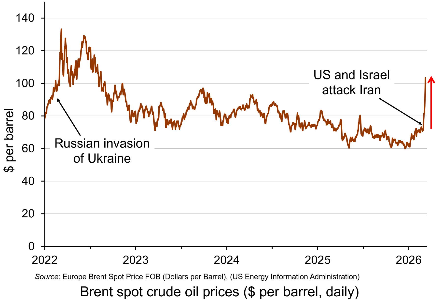
Oil prices rose considerably in the days following the start of the war on 28 February, with Brent crude, a key measure of international oil prices, rising from $71.3 on 27 February to a peak of $119.4 per barrel by the morning of 9 March – a rise of 67%. It was possible that they would rise even further in the short term. However, prices fell back substantially later on 9 March after G7 finance ministers declared that the group ‘stands ready’ to release oil from strategic reserves if needed. By late in the day, the price had fallen to around $90. (Click here for a PowerPoint of the chart.)
However, despite the announcement on 11 March that 32 countries had agreed to release 400m barrels of oil reserves, oil prices began rising again and reached $100 on 12 March after three tankers had been struck in the Gulf, two of them close to the Strait of Hormuz. With Iran pledging to keep the Strait closed, there were worries that the release of oil reserves would provide only temporary relief. Just over 20m barrels of oil normally pass through the Strait of Hormuz. The 400m barrels released from storage is the equivalent, therefore, of only 20 days’ worth of lost oil from the Gulf.
 Rising oil prices will drive up inflation. For those countries with a heavy dependence on Gulf oil, particularly countries in Asia, there could be significant supply problems. For oil exporters in the Persian Gulf, with tankers unable to traverse the Strait of Hormuz, the economic impact is huge. Oil exporters outside the Gulf, such as Russia, Norway and Canada, however, will gain from the higher prices. Clearly the size of these effects will depend on how long the conflict continues and how long the Strait of Hormuz remains closed.
And it is not just oil that is affected. Other products, such as liquified natural gas (LNG), petrochemicals, industrial materials, fertilizers, metals and minerals are transported through the Strait of Hormuz. Gulf countries import much of their food through the Strait.
Cuts in supplies of oil and other products represent an adverse supply shock. Such shocks push up prices (cost-push inflation), while adversely affecting aggregate output. This can lead to stagflation – a combination of higher inflation and stagnation or even falling output. Central banks with a simple mandate to keep inflation to a target are likely to raise interest rates, or at least delay in reducing them. In the USA, with a dual mandate of controlling inflation but also maximising employment, the response may be less deflationary, depending on the judgement of the Federal Reserve.
Uncertainty
 There is great uncertainty about how long the conflict will last. There is also a lack of clarity and consistency from the US administration about its war aims. This uncertainty has affected financial markets, which have seen considerable volatility. Stock markets have seen widespread falls, with airline, travel and AI-heavy stocks being particularly vulnerable.
If the war is concluded relatively swiftly, the economic effects could be relatively small. If the war continues, and especially if the Gulf countries are drawn further into the conflict and if the conflict spreads to other countries, the economic effects could be much more substantial. A prolonged conflict could see oil prices remaining above $100 per barrel, potentially increasing global inflation by 1 percentage point or more. This would slow or halt the move by central banks to cut rates and thereby reduce global economic growth – potentially, as we have seen, leading to stagflation.
Then there is the issue of a potential new international refugee crisis. If the economic and political system in Iran deteriorates rapidly, this could trigger a wave of migration to neighbouring countries, such as Turkey, already hosting large numbers of refugees. Many could seek sanctuary further afield in Europe, with several countries already facing a backlash against immigration. The political and economic effects of this on host countries could be significant – but as yet, highly uncertain.
Articles
- Assessing the global economic impact of the Middle East war
ING, Carsten Brzeski, Warren Patterson, James Knightley and Deepali Bhargava (5/3/26)
- How will the Iran war affect the global economy?
Chatham House, Neil Shearing (6/3/26)
- Iran war is latest threat to a global economy rattled by Trump
Aljazeera, John Power (7/3/26)
- Why an Iran war inflation shock could wreck global economic recovery
The Guardian, Phillip Inman and Kalyeena Makortoff (8/3/26)
- Why has the Iran war sparked fears of stagflation for the global economy?
The Guardian, Luca Ittimani (9/2/26)
- Why surging oil prices are a shock for the global economy – but not yet a crisis
The Conversation, Stella Huangfu (3/3/26)
- Why the price of oil matters more than you might think
BBC News, Natalie Sherman and Mitchell Labiak (10/3/26)
- Strait of Hormuz: Factsheet
IEA (February 2026)
- Strait of Hormuz: Gulf states’ food security is at immediate risk but wider shortages could push up consumer prices globally
The Conversation, Gokcay Balci and Ebru Surucu-Balci (4/3/26)
- Faisal Islam: Oil price spiral may be slowed but not stopped by G7 emergency move
BBC News, Faisal Islam (9/3/26)
- What on earth is going on with the oil price?
BBC News, Jemma Crew (12/3/26)
- Asia scrambles to confront energy crisis unleashed by Iran war – with no end in sight
The Guardian, Callum Jones (12/3/26)
- The grim choice facing the Trump administration: Economic or naval collapse?
CNN, Phil Mattingly and Zachary Cohen (9/3/26)
- How the Iran Conflict May Fuel a New International Refugee Crisis
Forbes, Andy J Semotiuk (5/3/26)
Data
Questions
- Who are the biggest gainers and losers from disruption to oil supplies from the Persian Gulf?
- Illustrate the effect of the current oil price shock on an aggregate demand and supply diagram (either static or dynamic).
- Why is the Iranian war likely to be less damaging to the European economy than the Ukrainian war has been?
- Why have AI-related stock prices been vulnerable to the uncertainty caused by the Iranian war?
- How are the Bank of England and the Federal Reserve Bank likely to respond to the rising price of oil and the broader economic effects of the war? Why might their responses be different?
- What is the likely impact of the Iranian war on global economic recovery?
- How might the Iranian war affect global economic alliances?
- How is the current oil price shock likely to affect the eurozone? Will it be different from the oil price shock that followed the Russian invasion of Ukraine?
- What are the likely economic effects of large-scale migration caused by the war?
 Unemployment in the UK reached its highest level in nearly five years at the close of 2025, according to new data from the Office for National Statistics. Figures show the unemployment rate rising to 5.2% in the three months to December, up slightly from 5.1% in the preceding quarter.
This marks the highest unemployment level since the pandemic, coinciding with a slowdown in wage growth and increasing speculation that interest rates may soon be lowered.
Youth unemployment
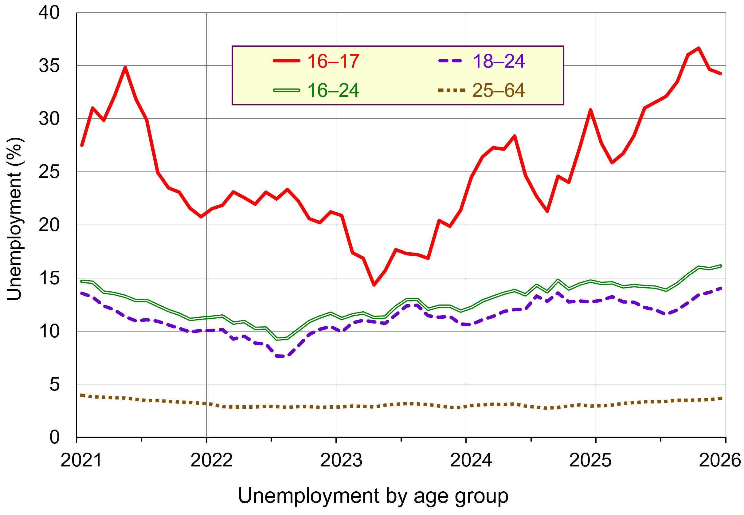 However, young people are taking the heaviest hit, with unemployment climbing to 16.1% among those aged 16 to 24. (Click here for a PowerPoint of the chart.) This is the highest level in more than a decade, including the spike seen during the pandemic. Economists largely attribute this trend to rising payroll costs, which they say are discouraging employers from offering entry level roles. Long-term youth unemployment is also worsening, with recent data showing that a growing share of unemployed young people have been out of work for over 12 months, highlighting deeper and more persistent barriers to re entry.
At the same time, although wages for those in work continue to grow faster than prices, the pace of wage growth is steadily slowing, adding further pressure on young people already facing the most challenging labour market conditions in years. According to ONS data, the annual growth in average weekly wages, excluding bonuses, slowed to 4.2% in the last three months of 2025. Private-sector wage growth eased to 3.4%, bringing it closer to the 3.25% rate that the Bank of England believes is consistent with its 2% inflation target.
The impact on interest rates
 The Bank of England is watching the slowdown in the UK jobs market closely as it gauges when next to lower its interest rates. In February 2026, the Monetary Policy Committee voted to hold the base rate (Bank Rate) at 3.75%. However, the committee voted with a majority of 5-4, with four members voting to reduce the rate to 3.5%.
The Bank of England uses interest rates as a policy tool to control inflation, the rate at which general prices rise in the economy. The current rate of inflation of 3.4% is above the Bank of England’s target of 2%.
In addition to the split vote, some economists believe that the easing in pay growth makes it likely that Bank Rate will be cut at the next meeting on 19th March. Paul Dales, chief UK economist at Capital Economics, said the fall in wage growth ‘supports the idea that the Bank of England has at least a couple more interest rate cuts in its locker’. A decrease in interest rates will be welcomed by investors.
What is behind the increase in youth unemployment?
Young people always tend to be the most impacted by a downturn in hiring. But economists warned that the rise in youth unemployment was a sign that employers are being more cautious about hiring younger workers. Openings for low-skilled entry-level roles and for new graduates have dropped steeply. Many businesses have slowed hiring due to an increase in costs because of measures in Chancellor Rachel Reeves’s last two Budgets. Businesses claim that the combination of increases in employer National Insurance contributions and a rise in the minimum wage mean they are facing higher payroll costs.
Peter Dixon at the National Institute for Economic and Social Research said, ‘there are indications that younger workers in particular are being priced out of the market’, supporting the explanation that raising the minimum wage might also be disincentivising the hiring of young people.
The ONS reported that the retail and wholesale sector saw the biggest fall in the number of workers on company payrolls, with 65,000 jobs lost in the sector since January last year. Meanwhile, health and social work saw the biggest rise in payrolled workers of any sector, adding 39,000 jobs in the year to January. Financial analyst at AJ Bell, Danni Hewson, suggested that those leaving the retail sector were now entering healthcare, with both sectors employing large numbers of women. However, she also warned that a recent surge in investment in artificial intelligence could hit young people the hardest as it could result ‘in a scarcity of entry level posts’ (see the blog Will AI make the world less equal?.
Job vacancies
 Job vacancy data across the UK indicates a significant cooling in labour demand. According to the latest ONS figures, vacancies fell from 736,000 in the three months to December to 726,000 in January, signalling continued weakening in hiring activity. According to the job search site, Adzuna, the number of vacant positions has dropped to its lowest level in five years, with job listings sliding 3% in January to 695,000, marking the first time vacancies have dipped below 700,000 since early 2021. Notably, graduate opportunities have fallen below 10,000 for the first time since Adzuna started tracking in 2016, underscoring the deepening challenges for new entrants to the workforce.
This downward trend in job openings extends patterns seen throughout late 2025, with vacancies down 16% from the previous January and nearly 20% lower than six months earlier. This coincides with a rise in unemployment to 5.2%, slower wage growth, and a growing concern that young people are disproportionately affected as hiring slows. As opportunities shrink, competition has intensified: there are now 2.4 jobseekers per vacancy, up from 2.27 in December, with the most sought-after roles including warehouse staff, healthcare support workers, lorry drivers, labourers and kitchen assistants.
How can the situation be improved?
Pat McFadden, Secretary for Work and Pensions, has commissioned the former Health Secretary Alan Milburn to lead a review into the causes of rising youth inactivity. There will be a particular focus on mental health issues that are pushing young people out of education and employment. This initiative responds to the growing number of young people not in education, employment, or training (NEETs), many of whom are now classified as inactive rather than unemployed. Some receive health-related benefits and are therefore not required to look for work, while others fall outside the benefits system entirely, making them harder to identify and support.
However, Pat McFadden said there was ‘more to do to get people into jobs’, and that tackling youth unemployment is a key government priority. He added that Labour was working to make it easier for young people to find and secure an apprenticeship, supported by a wider package of reforms. The reforms announced by McFadden include creating 50,000 additional apprenticeships. The government will also expand support for 350,000 people to move into work or training in sectors such as care and construction, with the risk of losing benefits if they refuse. They also include the provision of 55,000 state-funded, six-month work placements for the long-term unemployed.
While these measures are widely seen as necessary, campaign groups argue the government should go further by extending its ‘Youth Guarantee’ to cover all young people up to age 24, rather than ending at 22.
 However, as Alice Martin, head of research at Lancaster University’s Work Foundation, notes, initiatives designed to help people return to the labour market have limited impact ‘if the jobs aren’t out there.’ Even graduates are finding that opportunities are scarce, and for those leaving education with few qualifications, the situation is even more challenging. Sectors such as retail, once a reliable source of first jobs, have been in long-term structural decline, a trend that is now accelerating and further narrowing the pathways available to young people entering the workforce.
The situation has prompted government discussions about postponing the planned rise in the minimum wage for 18- to 20-year-olds to address employers’ concerns and encourage more youth employment. However, on Wednesday, Keir Starmer stressed that Labour remains committed to its manifesto pledge to align the pay of younger workers with that of older employees. The Prime Minister confirmed that the promise to ‘remove the discriminatory age bands’ in the minimum wage system still stands, and that the increase scheduled for April will proceed as planned.
Starmer said ‘We’ve made commitments to young people in our manifesto, and we will keep to those commitments, including the commitment that we would make sure that the living wage and minimum wage will go up this April, which we can absolutely confirm to you will happen.’
Unemployment outlook
Multiple economic forecasts predict that unemployment will to continue to rise in 2026. The most frequently cited projection places the 2026 unemployment rate around 5.2%–5.5%. However, some economists expect businesses to regain confidence and begin hiring again later in the year, supporting a gradual stabilisation in job markets.
Yet risks remain significant: if that recovery fails to materialise, unemployment could edge toward 6% by the end of the year, with forecasts from JP Morgan suggesting unemployment may reach 2 million in the first half as firms delay recruitment following the recent rise in the employers’ National Insurance rate. This environment is proving especially challenging for young people, with early career opportunities among the first to disappear and delayed entry into work potentially limiting long-term earnings and progression.
As hiring becomes more cautious and entry-level roles tighten, the path into the labour market risks becoming narrower, underscoring the need for policies and conditions that support both employer confidence and opportunities for new entrants.
Articles
FT Articles (subscribers only)
Data
Questions
- Explain why youth unemployment has risen more sharply than overall unemployment at the end of 2025.
- What are the costs to the individual of being unemployed?
- What are the wider non-monetary costs to society?
- Explain the main financial costs to the wider economy of a rising unemployment rate.
- Assess the likely impact of slowing wage growth on the Bank of England’s decision about whether or not to cut interest rates in early 2026.
- Discuss how falling job vacancies, particularly graduate and entry‑level opportunities, might affect long‑term labour market outcomes for young people.
- Evaluate the effectiveness of government policies such as expanding apprenticeships, increasing work placements, and reviewing youth inactivity in reducing youth unemployment.
 Donald Trump is keen to lower US interest rates substantially and rapidly in order to provide a boost to the US economy. He is also keen to reduce the cost of living for US citizens and sees lower interest rates as a means of reducing the burden of debt servicing for both consumers and firms alike.
But interest rates are set by the US central bank, the Federal Reserve (the ‘Fed’), which is formally independent from government. This independence is seen as important for providing stability to the US economy and removing monetary policy from short-term political pressures to cut interest rates. Succumbing to political pressures would be likely to create uncertainty and damage long-term stability and growth.
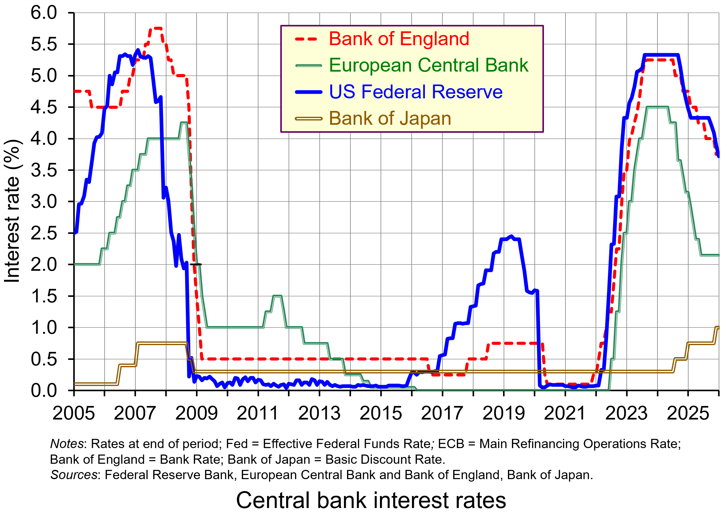
Yet President Trump is pushing the Fed to lower interest rates rapidly and despite three cuts in a row of 0.25 percentage points in the last part of 2025 (see chart below), he thinks this as too little and is annoyed by suggestions that the Fed is unlikely to lower rates again for a while. He has put great pressure on Jerome Powell, the Fed Chair, to go further and faster and has threatened to replace him before his term expires in May this year. He has also made clear that he is likely to appoint someone more willing to cutting rates.
The Federal Reserve headquarters in Washington is currently being renovated. The nine-year project is costing $2.5 billion and is due to be completed next year. President Trump has declared that the project’s costs are excessive and unnecessary.
On 11 January, Federal prosecutors confirmed that they were opening a criminal investigation into Powell, accusing him of lying to Congress in his June 2025 testimony regarding the scope and costs of the renovations.
Powell responded by posting a video in which he claimed that the real reason that he was being threatened with criminal charges was not because of the renovations but because the Fed had ignored President Trump’s pressure and had set interest rates:
based on our best assessment of what will serve the public, rather than following the preferences of the President. This is about whether the Fed will be able to continue to set interest rates based on evidence and economic conditions – or whether, instead, monetary policy will be directed by political pressure or intimidation.
The Fed’s mandate
 The Federal Reserve Board decides on monetary policy and then the Federal Open Market Committee (FOMC) decides how to carry it out. It decides on interest rates and asset sales or purchases. The FOMC meets eight times a year.
The Fed is independent of both the President and Congress, and its Chair is generally regarded as having great power in determining the country’s economic policy.
Since 1977, the Fed’s statutory mandate has been to promote the goals of stable prices and maximum employment. Because of the reference to both prices and employment, the mandate is commonly referred to as a ‘dual mandate’. Its inflation target is 2 per cent over the long run with ‘well anchored’ inflationary expectations.
The dual mandate is unlike that of the Bank of England, the European Central Bank, the Bank of Japan and most other central banks, which all have a single key mandate of achieving a target of a 2 per cent annual rate of consumer price inflation over a particular time period.
With a dual mandate, the two objectives may well conflict from time to time. Moreover, changes in monetary policy affect these objectives with a lag and potentially over different time horizons. Hence, an assessment may have to be made of which is the most pressing problem. This does give some leeway in setting interest rates somewhat lower than if there were a single inflation-rate target. Nevertheless, the assessment is in terms of how best to achieve the mandate and not to meet current political goals.
Statement by former Fed Chairs and Governors
On 12 January, three former Chairs of the Federal Reserve (Janet Yellen, Ben Bernanke and Alan Greenspan), four former Treasury Secretaries (Timothy Geithner, Jacob Lew, Henry Paulson and Robert Rubin) and seven other top former economic officials issued the following statement (see Substack link in the Articles section below):
The Federal Reserve’s independence and the public’s perception of that independence are critical for economic performance, including achieving the goals Congress has set for the Federal Reserve of stable prices, maximum employment, and moderate long-term interest rates. The reported criminal inquiry into Federal Reserve Chair Jay Powell is an unprecedented attempt to use prosecutorial attacks to undermine that independence. This is how monetary policy is made in emerging markets with weak institutions, with highly negative consequences for inflation and the functioning of their economies more broadly. It has no place in the United States whose greatest strength is the rule of law, which is at the foundation of our economic success.
Response of investors
 What will happen to the dollar, US bond prices, share prices and US inflation, and what will happen to investment, depends on how people respond to the threat to the Fed’s independence. Initially, there was little response from markets, with investors probably concluding that President Trump is unlikely to be able to sway FOMC members. What is more, several Republican lawmakers have begun criticising the Trump administration’s criminal investigation, making it harder for the President to influence Fed decisions.
Even if Powell is replaced, either in the short term or in May, by a chair keen to pursue the Trump agenda, that chair will still be just one of twelve voting members of the FOMC.
Seven are appointed by the President, but serve for staggered 14-year terms. Four have been appointed by President Trump, but the other three were appointed by President Biden, although one – Lisa Cook – is being indicted by the Supreme Court for mortgage fraud, with the hearing scheduled for January 21. She claims that this is a trumped-up charge to provide grounds for removing her from the Fed. If she is removed, President Trump could appoint a replacement minded to cut rates.
The other five members include the President of the New York Fed and four of the eleven other regional Fed Presidents serving in rotation. These four are generally hawkish and would oppose early rate cuts.
Thus it is unlikely that President Trump will succeed in pushing the Fed to lower interest rates earlier than they would have done. For that reason, markets have remained relatively sanguine.
 Nevertheless, Donald Trump’s actions could well cause investors to become more worried. Will he try to find other ways to undermine the Fed? Will his actions over Venezuela, Cuba, Greenland and Iran, let alone his policies towards Ukraine and Russia and towards Israel and Gaza, heighten global uncertainty? Will his actions towards Venezuela and his desire to take over Greenland embolden China to attempt to annex Taiwan, and Russia to continue to resist plans to end the war in Ukraine or to make stronger demands?
Such developments could cause investor confidence to wane and for stock markets to fall. Time will tell. I think we need a crystal ball!
Videos
Articles
- Federal prosecutors open criminal investigation into the Fed and Jerome Powell
CNN, Bryan Mena (11/1/26)
- The Fed just gave a rare look at its $2.5 billion renovation — right before Trump’s tour
CNN, Bryan Mena (24/7/25)
- ‘A bone-headed move’: Trump’s shocking battle with Powell could badly backfire
CNN, Matt Egan (12/1/26)
- Why Powell is fighting back against Trump: The US economy is at stake
CNN, Bryan Mena (13/1/26)
- Fed chair Powell hits out at ‘unprecedented’ probe by US justice department
BBC News, Ana Faguy and Osmond Chia (12/1/26)
- Justice department opens investigation into Jerome Powell as Trump ramps up campaign against Federal Reserve
The Guardian, Callum Jones (12/1/26)
- Some Republicans speak out against DoJ investigation into Fed chair
The Guardian, Joseph Gedeon (12/1/26)
- Trump’s attempts to influence Fed risk 1970s-style inflation and global backlash
The Guardian, Richard Partington (12/1/26)
- Statement on the Federal Reserve
Substack, 14 signatories (12/1/26)
- Yellen says Powell probe ‘extremely chilling’ for Fed independence, market should be concerned
CNBC, Jeff Cox (12/1/26)
- Global central bankers unite in defense of Fed Chair Jerome Powell
CNBC, Holly Ellyatt (13/1/26)
- Trump attacks Powell again amid Fed independence fears: ‘That jerk will be gone soon’
CNBC, Kevin Breuninger (13/1/26)
- Former Fed chairs condemn criminal investigation into Jerome Powell
BBC News, Danielle Kaye (12/1/26)
- Fed: Towards a very divided Fed in the coming months and quarters
CPR AM, Bastien Drut (28/11/25)
- Treasury Yields Diverge as Powell Probe Rekindles Fed Independence Risk
Investing.com, Khasay Hashimov (12/1/26)
- Instant View: Investors react as Trump-Fed feud escalates
Reuters (12/1/26)
- Fighting the Fed, Trump tries credit easing by decree
Reuters, Mike Dolan (13/1/26)
- Trump’s attacks on the Federal Reserve risk fuelling US inflation and ending dollar dominance
The Conversation, Emre Tarim (13/1/26)
Questions
- What are the arguments for central bank independence?
- What are the arguments for control of monetary policy by the central government?
- Assess the above arguments.
- Find out what has happened to interest rates, the US stock market and the dollar since this blog was written.
- How do the fiscal decisions by government affect monetary policy?
- Compare the benefits of the dual mandate system of the Fed with those of the single mandate of the Bank of England and ECB.
 With businesses increasing their use of AI, this is likely to have significant effects on employment. But how will this affect the distribution of income, both within countries and between countries?
In some ways, AI is likely to increase inequality within countries as it displaces low-skilled workers and enhances the productivity of higher-skilled workers. In other ways, it could reduce inequality by allowing lower-skilled workers to increase their productivity, while displacing some higher-skilled workers and managers through the increased adoption of automated processes.
The effect of AI on the distribution of income between countries will depend crucially on its accessibility. If it is widely available to low-income countries, it could significantly enhance the productivity of small businesses and workers in such countries and help to reduce the income gap with the richer world. If the gains in such countries, however, are largely experienced by multinational companies, whether in mines and plantations, or in labour-intensive industries, such as garment production, few of the gains may accrue to workers and global inequality may increase.
Redistribution within a country
 The deployment of AI may result in labour displacement. AI is likely to replace both manual and white-collar jobs that involve straightforward and repetitive tasks. These include: routine clerical work, such as data entry, filing and scheduling; paralegal work, contract drafting and legal research; consulting, business research and market analysis; accounting and bookkeeping; financial trading; proofreading, copy mark-up and translation; graphic design; machine operation; warehouse work, where AI-enabled warehouse robots do many receiving, sorting, stacking, retrieval, carrying and loading tasks (e.g. Amazon’s Sequoia robotic system); basic coding or document sifting; market research and advertising design; call-centre work, such as enquiry handling, sales, telemarketing and customer service; hospitality reception; sales cashiers in supermarkets and stores; analysis of health data and diagnosis. Such jobs can all be performed by AI assistants, AI assisted robots or chat bots.
Women are likely to be disproportionately affected because they perform a higher share of the administrative and service roles most exposed to AI.
Workers displaced by AI may find that they can find employment only in lower-paid jobs. Examples include direct customer-facing roles, such as bar staff, shop assistants, hairdressers and nail and beauty consultants.
Such job displacement by AI is likely to redistribute income from relatively low-skilled labour to capital: a redistribution from wages to profits. This will tend to lead to greater inequality.
AI is also likely to lead to a redistribution of income towards certain types of high-skilled labour that are difficult to replace with AI but which could be enhanced by it. Take the case of skilled traders, such as plumbers, electricians and carpenters. They might be able to use AI in their work to enhance their productivity, through diagnosis, planning, problem-solving, measurement, etc. but the AI would not displace them. Instead, it could increase their incomes by allowing them to do their work more efficiently or effectively and thus increase their output per hour and enhance their hourly reward. Another example is architecture, where AI can automate repetitive tasks and open up new design possibilities, allowing architects to focus on creativity, flexibility, aesthetics, empathy with clients and ethical decision-making.
An important distinction is between disembodied and embodied AI investment. Disembodied AI investment could include AI ‘assistants’, such as ChatGPT and other software that can be used in existing jobs to enhance productivity. Such investment can usually be rolled out relatively quickly. Although the extra productivity may allow some reduction in the number of workers, disembodied AI investment is likely to be less disruptive than embodied AI investment. The latter includes robotics and automation, where workers are replaced by machines. This would require more investment and may be slower to be adopted.
Then there are jobs that will be created by AI. These include prompt engineers, who develop questions and prompt techniques to optimise AI output; health tech experts, who help organisations implement new medical AI products; AI educators, who train people in the uses of AI in the workplace; ethics advisors, who help companies ensure that their uses of AI are aligned with their values, responsibilities and goals; and cybersecurity experts who put systems in place to prevent AI stealing sensitive information. Such jobs may be relatively highly paid.
 In other cases, the gains from AI in employment are likely to accrue mainly to the consumer, with probably little change in the incomes of the workers themselves. This is particularly the case in parts of the public sector where wages/salaries are only very loosely related to productivity and where a large part of the work involves providing a personal service. For example, health professionals’ productivity could be enhanced by AI, which could allow faster and more accurate diagnosis, more efficient monitoring and greater accuracy in surgery. The main gainers would be the patients, with probably little change in the incomes of the health professionals themselves. Teachers’ productivity could be improved by allowing more rapid and efficient marking, preparation of materials and record keeping, allowing more time to be spent with students. Again, the main gainers would be the students, with little change in teachers’ incomes. Other jobs in this category include social workers, therapists, solicitors and barristers, HR specialists, senior managers and musicians.
Thus there is likely to be a distribution away from lower-skilled workers to both capital and higher-skilled workers who can use AI, to people who work in new jobs created by AI and to the consumers of certain services.
AI will accelerate productivity growth and, with it, GDP growth, but will probably displace workers faster than new roles emerge. This is likely to increase inequality and be a major challenge for society. Can the labour market adapt? Could the effects be modified if people moved to a four- or three-day week? Will governments introduce statutory limits to weekly working hours? Will training and education adapt to the new demands of employers?
Redistribution between countries
 AI threatens to widen the global rich–poor divide. It will give wealthier nations a productivity and innovation edge, which could displace low-skilled jobs in low-income nations. Labour-intensive production could be replaced by automated production, with the capital owned by the multinational companies of just a few countries, such as the USA and China, which between them account for 40% of global corporate AI R&D spending. For some companies, it would make sense to relocate production to rich countries, or certain wealthier developing countries, with better digital infrastructure, advanced data systems and more reliable power supply.
For other companies, however, production might still be based in low-income countries to take advantage of low-cost local materials. But there would still be a redistribution from wages in such countries to the profits of multinationals.
But it is not just in manufacturing where low-income countries are vulnerable to the integration of AI. Several countries, such as India, the Philippines, Mexico and Egypt have seen considerable investment in call centres and IT services for business process outsourcing and customer services. AI now poses a threat to employment in this industry as it has the potential to replace large numbers of workers.
AI-related job losses could exacerbate unemployment and deepen poverty in poorer countries, which, with limited resources, limited training and underdeveloped social protection systems, are less equipped to absorb economic and social shocks. This will further widen the global divide. In the case of embodied AI investment, it may only be possible in low-income countries through multinational investment and could displace many traditional jobs, with much of the benefit going in additional multinational profit.
But it is not all bad news for low-income countries. AI-driven innovations in healthcare, education, and agriculture, if adopted in poor countries, can make a significant contribution to raising living standards and can slow, or even reverse, the widening gap between rich and poor nations. Some of the greatest potential is in small-scale agriculture. Smallholders can boost crop yields though precision farming powered by AI; AI tools can help farmers buy seeds, fertilisers and animals and sell their produce at optimum times and prices; AI-enabled education tools can help farmers learn new techniques.
Articles
- New Skills and AI Are Reshaping the Future of Work
IMF Blog, Kristalina Georgieva (14/1/26)
- Generative AI: degenerative for jobs?
Bank Underground, Bank of England blog, Edward Egan (22/1/26)
- Artificial intelligence (AI) and employment
UK Parliament Research Briefing Lydia Harriss and Sam Money-Kyrle (23/12/25)
- Is Your Job AI-Proof? What to Know About AI Taking Over Jobs
Built In, Matthew Urwin (27/8/25)
- AI likely to displace jobs, says Bank of England governor
BBC News, Michael Race (19/12/25)
- These Jobs Will Fall First as AI Takes Over the Workplace
Forbes, Jack Kelly (30/4/25)
- Disrupted or displaced? How AI is shaking up jobs
exec-appointments.com, Anjli Raval (9/7/25)
- Navigate the economic risks and challenges of generative AI
EY-Parthenon, Lydia Boussour (25/6/24)
- AI Isn’t Increasing Inequality; It’s Revealing the Gaps We Haven’t Wanted to See
HR News, Mark Abbott (18/12/25)
- AI promises efficiency, but it’s also amplifying labour inequality
The Conversation, Mehnaz Rafi (3/12/25)
- 10 Jobs AI Will Replace in 2025
Live Career, Marta Bongilaj (29/12/25)
- From steam to Silicon: Why inequality persists
Aik News HD (Pakistan), Ahmed Fawad Farooq (27/12/25)
- Rethinking AI’s role in income inequality
PwC: The Leadership Agenda (4/9/25)
- How Europe Can Capture the AI Growth Dividend
IMF Blog, Florian Misch, Ben Park, Carlo Pizzinelli and Galen Sher (20/11/25)
- The Next Great Divergence
UNDP: Asia and the Pacific (2/12/25)
- AI risks sparking a new era of divergence as development gaps between countries widen, UNDP report finds
UNDP Press Release (2/12/25)
- AI threatens to widen inequality among states: UN
Aljazeera (2/12/25)
- AI risks deepening inequality, says head of world’s largest SWF
Financial Times, James Fontanella-Khan and Sun Yu (23/11/25)
- Three Reasons Why AI May Widen Global Inequality
Center for Global Development, Philip Schellekens and David Skilling (17/10/24)
- AI Will Transform the Global Economy. Let’s Make Sure It Benefits Humanity
IMF Blog, Kristalina Georgieva (14/1/24)
- AI’s $4.8 trillion future: UN Trade and Development alerts on divides, urges action
UNCTAD Press Release (7/4/25)
- AI could affect 40% of jobs and widen inequality between nations, UN warns
CNBC, Dylan Butts (4/4/25)
Questions
- What types of job are most vulnerable to AI?
- How will AI change the comparative advantage of low-income countries and what effect will it be likely to have on the pattern of global trade?
- Assess alternative policies that governments in high-income countries can adopt to offset the growth in inequality caused by the increasing use of AI.
- What policies can governments in low-income countries or aid agencies adopt to offset the growth in inequality within low-income countries and between high- and low-income countries?
- How might the growth of AI affect your own approach to career development?
- Is AI likely to increase or decrease economic power? Explain.
 We continue to live through incredibly turbulent times. In the past decade or so we have experienced a global financial crisis, a global health emergency, seen the UK’s departure from the European Union, and witnessed increasing levels of geopolitical tension and conflict. Add to this the effects from the climate emergency and it easy to see why the issue of economic uncertainty is so important when thinking about a country’s economic prospects.
In this blog we consider how we can capture this uncertainty through a World Uncertainty Index and the ways by which economic uncertainty impacts on the macroeconomic environment.
World Uncertainty Index
Hites Ahir, Nicholas Bloom and Davide Furceri have constructed a measure of uncertainty known as the World Uncertainty Index (WUI). This tracks uncertainty around the world using the process of ‘text mining’ the country reports produced by the Economist Intelligence Unit. The words searched for are ‘uncertain’, ‘uncertainty’ and ‘uncertainties’ and a tally is recorded based on the number of times they occur per 1000 words of text. To produce the index this figure is then multiplied up by 100 000. A higher number therefore indicates a greater level of uncertainty. For more information on the construction of the index see the 2022 article by Ahir, Bloom and Furceri linked below.
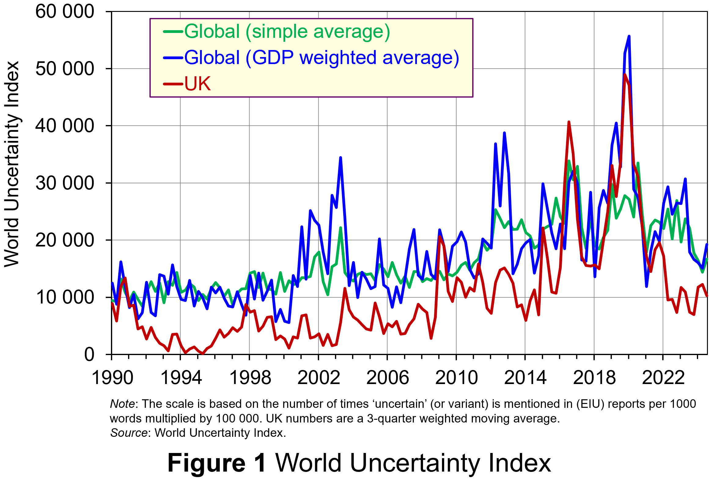 Figure 1 (click here for a PowerPoint) shows the WUI both globally and in the UK quarterly since 1991. The global index covers 143 countries and is presented as both a simple average and a GDP weighted average. The UK WUI is also shown. This is a three-quarter weighted average, the authors’ preferred measure for individual countries, where increasing weights of 0.1, 0.3 and 0.6 are used for the three most recent quarters.
From Figure 1 we can see how the level of uncertainty has been particularly volatile over the past decade or more. Events such as the sovereign debt crisis in parts of Europe in the early 2010s, the Brexit referendum in 2016, the COVID-pandemic in 2020–21 and the invasion of Ukraine in 2022 all played their part in affecting uncertainty domestically and internationally.
Uncertainty, risk-aversion and aggregate demand
Now the question turns to how uncertainty affects economies. One way of addressing this is to think about ways in which uncertainty affects the choices that people and businesses make. In doing so, we could think about the impact of uncertainty on components of aggregate demand, such as household consumption and investment, or capital expenditures by firms.
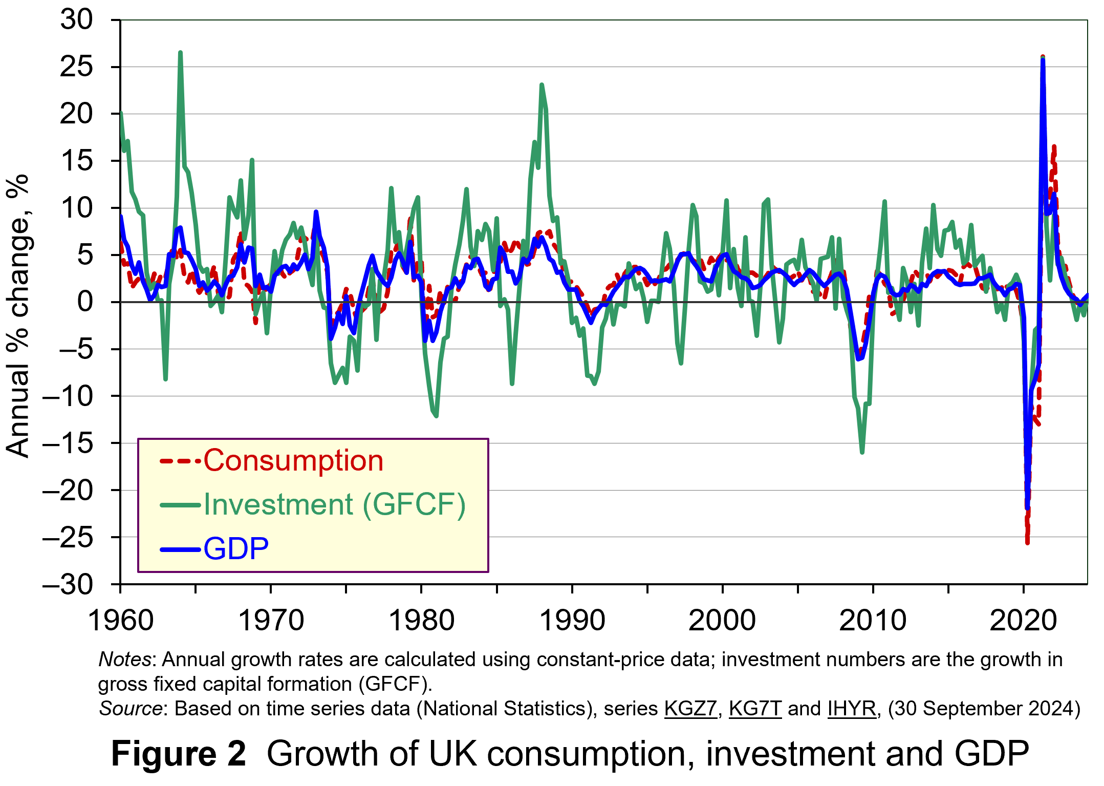 As Figure 2 shows (click here for a PowerPoint), investment is particularly volatile, and much more so than household spending. Some of this can be attributed to the ‘lumpiness’ of investment decisions since these expenditures tend to be characterised by indivisibility and irreversibility. This means that they are often relatively costly to finance and are ‘all or nothing’ decisions. In the context of uncertainty, it can make sense therefore for firms to wait for news that makes the future clearer. In this sense, we can think of uncertainty rather like a fog that firms are peering through. The thicker the fog, the more uncertain the future and the more cautious firms are likely to be.
The greater caution that many firms are likely to adopt in more uncertain times is consistent with the property of risk-aversion that we often attribute to a range of economic agents. When applied to household spending decisions, risk-aversion is often used to explain why households are willing to hold a buffer stock of savings to self-insure against unforeseen events and their future financial outcomes being worse than expected. Hence, in more uncertain times households are likely to want to increase this buffer further.
 The theory of buffer-stock saving was popularised by Christopher Carroll in 1992 (see link below). It implies that in the presence of uncertainty, people are prepared to consume less today in order to increase levels of saving, pay off existing debts, or borrow less relative to that in the absence of uncertainty. The extent of the buffer of financial wealth that people want to hold will depend on their own appetite for risk, the level of uncertainty, and the moderating effect from their own impatience and, hence, present bias for consuming today.
Risk aversion is consistent with the property of diminishing marginal utility of income or consumption. In other words, as people’s total spending volumes increase, their levels of utility or satisfaction increase but at an increasingly slower rate. It is this which explains why individuals are willing to engage with the financial system to reallocate their expected life-time earnings and have a smoother consumption profile than would otherwise be the case from their fluctuating incomes.
Yet diminishing marginal utility not only explains consumption smoothing, but also why people are willing to engage with the financial system to have financial buffers as self-insurance. It explains why people save more or borrow less today than suggested by our base-line consumption smoothing model. It is the result of people’s greater dislike (and loss of utility) from their financial affairs being worse than expected than their like (and additional utility) from them being better than expected. This tendency is only likely to increase the more uncertain times are. The result is that uncertainty tends to lower household consumption with perhaps ‘big-ticket items’, such as cars, furniture, and expensive electronic goods, being particularly sensitive to uncertainty.
Uncertainty and confidence
Uncertainty does not just affect risk; it also affects confidence. Risk and confidence are often considered together, not least because their effects in generating and transmitting shocks can be difficult to disentangle.
We can think of confidence as capturing our mood or sentiment, particularly with respect to future economic developments. Figure 3 plots the Uncertainty Index for the UK alongside the OECD’s composite consumer and business confidence indicators. Values above 100 for the confidence indicators indicate greater confidence about the future economic situation and near-term business environment, while values below 100 indicate pessimism towards the future economic and business environments.
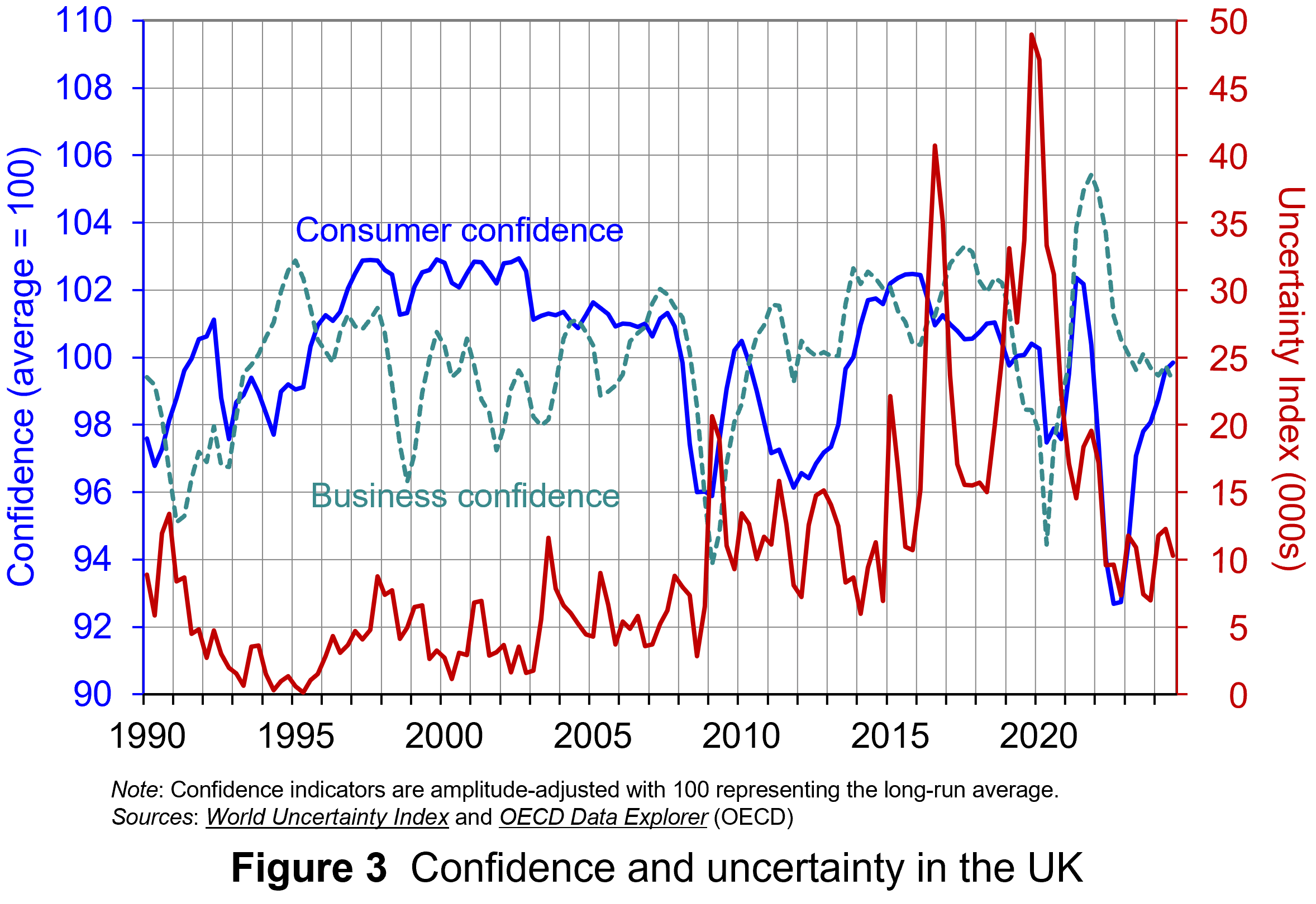 Figure 3 suggests that the relationship between confidence and uncertainty is rather more complex than perhaps is generally understood (click here for a PowerPoint). Haddow, Hare, Hooley and Shakir (see link below) argue that the evidence tends to point to changes in uncertainty affecting confidence, but with less evidence that changes in confidence affect uncertainty.
To illustrate this, consider the global financial crisis of the late 2000s. The argument can be made that the heightened uncertainty about future prospects for households and businesses helped to erode their confidence in the future. The result was that people and businesses revised down their expectations of the future (pessimism). However, although people were more pessimistic about the future, this was more likely to have been the result of uncertainty rather than the cause of further uncertainty.
Conclusion
For economists and policymakers alike, indicators of uncertainty, such as the Ahir, Bloom and Furceri World Uncertainty Index, are invaluable tools in understanding and forecasting behaviour and the likely economic outcomes that follow. Some uncertainty is inevitable, but the persistence of greater uncertainty since the global financial crisis of the late 2000s compares quite starkly with the relatively lower and more stable levels of uncertainty seen from the mid-1990s up to the crisis. Hence the recent frequency and size of changes in uncertainty show how important it to understand how uncertainty effects transmit through economies.
Academic papers
- The World Uncertainty Index
National Bureau of Economic Research, Working Paper 29763, Hites Ahir, Nicholas Bloom and Davide Furceri (February 2022)
- The Buffer-Stock Theory of Saving: Some Macroeconomic Evidence
Brookings Papers on Economic Activity, Christopher D Carroll (Vol 2, 1992)
- Macroeconomic uncertainty: what is it, how can we measure it and why does it matter?
Bank of England Quarterly Bulletin, 2013 Q2, Abigail Haddow, Chris Hare, John Hooley and Tamarah Shakir (13/6/13)
Articles
Data
Questions
- (a) Explain what is meant by the concept of diminishing marginal utility of consumption.
(b) Explain how this concept helps us to understand both consumption smoothing and the motivation to engage in buffer-stock saving.
- Explain the distinction between confidence and uncertainty when analysing macroeconomic shocks.
- Discuss which types of expenditures you think are likely to be most susceptible to uncertainty shocks.
- Discuss how economic uncertainty might affect productivity and the growth of potential output.
- How might the interconnectedness of economies affect the transmission of uncertainty effects through economies?
 With relentless bombing of Iran by Israel and the USA, and with Iranian counterattacks on Gulf states, the costs of the war are mounting. The most obvious are in terms of human lives, injuries and suffering. But there are significant economic costs too. Some of these are immediate, such as the rising price of oil and hence the costs of fuel, or the fall in stock market prices. Some will be longer term, depending on how the war develops. For example, prices could rise more generally as supply chains are disrupted.
 The impacts will vary across the world and across markets. The most obvious markets to be affected are those where significant supply comes from the Persian Gulf. Approximately 20% of total global oil consumption passes through the Strait of Hormuz, which connects the Persian Gulf with the Arabian Sea and the Indian Ocean.
 Rising oil prices will drive up inflation. For those countries with a heavy dependence on Gulf oil, particularly countries in Asia, there could be significant supply problems. For oil exporters in the Persian Gulf, with tankers unable to traverse the Strait of Hormuz, the economic impact is huge. Oil exporters outside the Gulf, such as Russia, Norway and Canada, however, will gain from the higher prices. Clearly the size of these effects will depend on how long the conflict continues and how long the Strait of Hormuz remains closed.
 There is great uncertainty about how long the conflict will last. There is also a lack of clarity and consistency from the US administration about its war aims. This uncertainty has affected financial markets, which have seen considerable volatility. Stock markets have seen widespread falls, with airline, travel and AI-heavy stocks being particularly vulnerable.
 Unemployment in the UK reached its highest level in nearly five years at the close of 2025, according to new data from the Office for National Statistics. Figures show the unemployment rate rising to 5.2% in the three months to December, up slightly from 5.1% in the preceding quarter.
 However, young people are taking the heaviest hit, with unemployment climbing to 16.1% among those aged 16 to 24. (Click
  The Bank of England is watching the slowdown in the UK jobs market closely as it gauges when next to lower its interest rates. In February 2026, the Monetary Policy Committee voted to hold the base rate (Bank Rate) at 3.75%. However, the committee voted with a majority of 5-4, with four members voting to reduce the rate to 3.5%.
  Job vacancy data across the UK indicates a significant cooling in labour demand. According to the latest ONS figures, vacancies fell from 736,000 in the three months to December to 726,000 in January, signalling continued weakening in hiring activity. According to the job search site, Adzuna, the number of vacant positions has dropped to its lowest level in five years, with job listings sliding 3% in January to 695,000, marking the first time vacancies have dipped below 700,000 since early 2021. Notably, graduate opportunities have fallen below 10,000 for the first time since Adzuna started tracking in 2016, underscoring the deepening challenges for new entrants to the workforce.
 However, as Alice Martin, head of research at Lancaster University’s Work Foundation, notes, initiatives designed to help people return to the labour market have limited impact ‘if the jobs aren’t out there.’ Even graduates are finding that opportunities are scarce, and for those leaving education with few qualifications, the situation is even more challenging. Sectors such as retail, once a reliable source of first jobs, have been in long-term structural decline, a trend that is now accelerating and further narrowing the pathways available to young people entering the workforce.
 Donald Trump is keen to lower US interest rates substantially and rapidly in order to provide a boost to the US economy. He is also keen to reduce the cost of living for US citizens and sees lower interest rates as a means of reducing the burden of debt servicing for both consumers and firms alike.
 The Federal Reserve Board decides on monetary policy and then the Federal Open Market Committee (FOMC) decides how to carry it out. It decides on interest rates and asset sales or purchases. The FOMC meets eight times a year.
  What will happen to the dollar, US bond prices, share prices and US inflation, and what will happen to investment, depends on how people respond to the threat to the Fed’s independence. Initially, there was little response from markets, with investors probably concluding that President Trump is unlikely to be able to sway FOMC members. What is more, several Republican lawmakers have begun criticising the Trump administration’s criminal investigation, making it harder for the President to influence Fed decisions.
 Nevertheless, Donald Trump’s actions could well cause investors to become more worried. Will he try to find other ways to undermine the Fed? Will his actions over Venezuela, Cuba, Greenland and Iran, let alone his policies towards Ukraine and Russia and towards Israel and Gaza, heighten global uncertainty? Will his actions towards Venezuela and his desire to take over Greenland embolden China to attempt to annex Taiwan, and Russia to continue to resist plans to end the war in Ukraine or to make stronger demands?
 With businesses increasing their use of AI, this is likely to have significant effects on employment. But how will this affect the distribution of income, both within countries and between countries?
 The deployment of AI may result in labour displacement. AI is likely to replace both manual and white-collar jobs that involve straightforward and repetitive tasks. These include: routine clerical work, such as data entry, filing and scheduling; paralegal work, contract drafting and legal research; consulting, business research and market analysis; accounting and bookkeeping; financial trading; proofreading, copy mark-up and translation; graphic design; machine operation; warehouse work, where AI-enabled warehouse robots do many receiving, sorting, stacking, retrieval, carrying and loading tasks (e.g. Amazon’s Sequoia robotic system); basic coding or document sifting; market research and advertising design; call-centre work, such as enquiry handling, sales, telemarketing and customer service; hospitality reception; sales cashiers in supermarkets and stores; analysis of health data and diagnosis. Such jobs can all be performed by AI assistants, AI assisted robots or chat bots.
 In other cases, the gains from AI in employment are likely to accrue mainly to the consumer, with probably little change in the incomes of the workers themselves. This is particularly the case in parts of the public sector where wages/salaries are only very loosely related to productivity and where a large part of the work involves providing a personal service. For example, health professionals’ productivity could be enhanced by AI, which could allow faster and more accurate diagnosis, more efficient monitoring and greater accuracy in surgery. The main gainers would be the patients, with probably little change in the incomes of the health professionals themselves. Teachers’ productivity could be improved by allowing more rapid and efficient marking, preparation of materials and record keeping, allowing more time to be spent with students. Again, the main gainers would be the students, with little change in teachers’ incomes. Other jobs in this category include social workers, therapists, solicitors and barristers, HR specialists, senior managers and musicians.
 AI threatens to widen the global rich–poor divide. It will give wealthier nations a productivity and innovation edge, which could displace low-skilled jobs in low-income nations. Labour-intensive production could be replaced by automated production, with the capital owned by the multinational companies of just a few countries, such as the USA and China, which between them account for 40% of global corporate AI R&D spending. For some companies, it would make sense to relocate production to rich countries, or certain wealthier developing countries, with better digital infrastructure, advanced data systems and more reliable power supply.
 We continue to live through incredibly turbulent times. In the past decade or so we have experienced a global financial crisis, a global health emergency, seen the UK’s departure from the European Union, and witnessed increasing levels of geopolitical tension and conflict. Add to this the effects from the climate emergency and it easy to see why the issue of economic uncertainty is so important when thinking about a country’s economic prospects.
 Figure 1 (click
  As Figure 2 shows (click
  The theory of buffer-stock saving was popularised by Christopher Carroll in 1992 (see link below). It implies that in the presence of uncertainty, people are prepared to consume less today in order to increase levels of saving, pay off existing debts, or borrow less relative to that in the absence of uncertainty. The extent of the buffer of financial wealth that people want to hold will depend on their own appetite for risk, the level of uncertainty, and the moderating effect from their own impatience and, hence, present bias for consuming today.
 Figure 3 suggests that the relationship between confidence and uncertainty is rather more complex than perhaps is generally understood (click