 The following blog is inspired by my teaching of macroeconomic issues to my final year students at Aston University. In the classes we’ve been discussing important aspects of monetary and fiscal policy design. What has become clear to me and my students is that the trade-offs which characterise the discipline of economics are certainly alive and well in the current environment in which monetary and fiscal policy choices are being made.
To demonstrate this we consider here some of the discussions we’ve had in class around central bank independence and monetary policy mandates. We’ve also looked at fiscal policy. Here we’ve examined the state of the public finances and the importance that seems to be attached to debt stabilisation and the imposition of debt rules.
Delegation and central bank mandates
My teaching this term began by introducing my students to one of the most important and influential monetary policy models. This is the model of Kydland and Prescott. Their model, published in the Journal of Political Economy in 1977 has become the theoretical bedrock for the modern-day operational independence of central banks.1
 The model explores how systemically high inflation can become established in economies when policymakers have the political incentive to lower unemployment or increase output above its long-run equilibrium value. This may be the case if governments operate monetary policy rather than the central bank (of if the central bank operates monetary policy but follows government objectives). By adopting expansionary monetary policy, governments can increase their popularity.
But this is likely to be short-lived, as any increased economic activity will only be temporary (assuming that the natural-rate hypothesis holds). Soon, inflation will rise.
But, if an election is on the horizon, there may be enough time to boost output and employment before inflation rises. In other words, an expectations-augmented Phillips curve may present governments with an incentive to loosen monetary policy and worry about the inflation consequences after the election.
However, the resulting ‘inflation surprise’ through the loosening of monetary policy means a fall in real pay and therefore in purchasing power. If people suspect that governments will be tempted to loosen policy, they will keep their expectations of inflation higher than the socially optimal inflation rate. Consequently, low-inflation targets lack credibility when governments have the temptation to loosen monetary policy. Such targets are time-inconsistent because governments have an incentive to renege and deliver higher inflation through a looser monetary policy. The result is an inflation bias.
Central bank independence
To prevent this inflationary bias arising, many central banks around the world have been given some form of operational independence with a mandate centred around an inflation-rate target. By delegating monetary policy to a more conservative central bank, the problem of inflationary bias can be addressed.
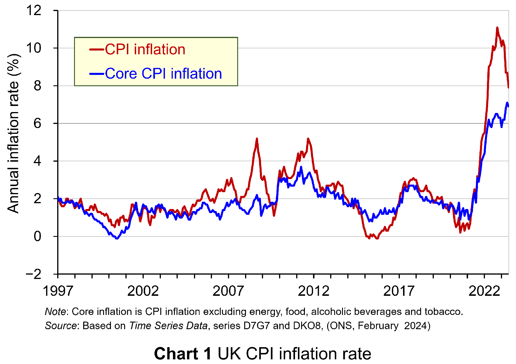 Yet central bank independence is not without its own issues and this has been an important part of the discussions with my students. Today, many economies are continuing to experience the effects of the inflationary shocks that began in 2021 (see Chart 1 for the UK CPI inflation rate: click here for a PowerPoint). The question is whether the appointment of a conservative or hard-nosed hawkish central banker trades off the stabilisation of inflation for greater volatility in output or unemployment.
The inflation–output stabilisation trade-off is closely associated with the works of Kenneth Rogoff2 and John Taylor3. The latter is known for his monetary policy rule, which has become known as the ‘Taylor rule’. This advocates that a rules-based central bank ought to place weight on both inflation and output stabilisation.
This is not without its own issues, however, since, by also placing weight on output stabilisation, we are again introducing the possibility of greater inflationary bias in policy making. Hence, while the act of delegation and a rules- or target-based approach may mitigate the extent of the bias relative to that in the Kydland and Prescott model, there nonetheless still remain issues around the design of the optimal framework for the conduct of monetary policy.
Indeed, the announcement that the UK had moved into recession in the last two quarters of 2023 can be seen as evidence that an otherwise abstract theoretical trade-off between inflation and output stabilisation is actually very real.
My classroom discussions have also shown how economic theory struggles to identify an optimal inflation-rate target. Beyond accepting that a low and stable inflation rate is desirable, it is difficult to address fully the student who asks what is so special about a 2% inflation target. Would not a 3% target, for example, be preferable, they might ask?
Whilst this may sound somewhat trivial, it has real-world consequences. In a world that now seems to be characterised by greater supply-side volatility and by more frequent inflation shocks than we were used to in recent history, might a higher inflation rate target be preferable? Certainly, one could argue that, with an inflation–output stabilisation trade-off, there is the possibility that monetary policy could be unduly restrictive in our potential new macroeconomic reality. Hence, we might come to see governments and central banks in the near future revisiting the mandates that frame the operation of their monetary policy. Time will tell.
Fiscal policy and debt stabilisation
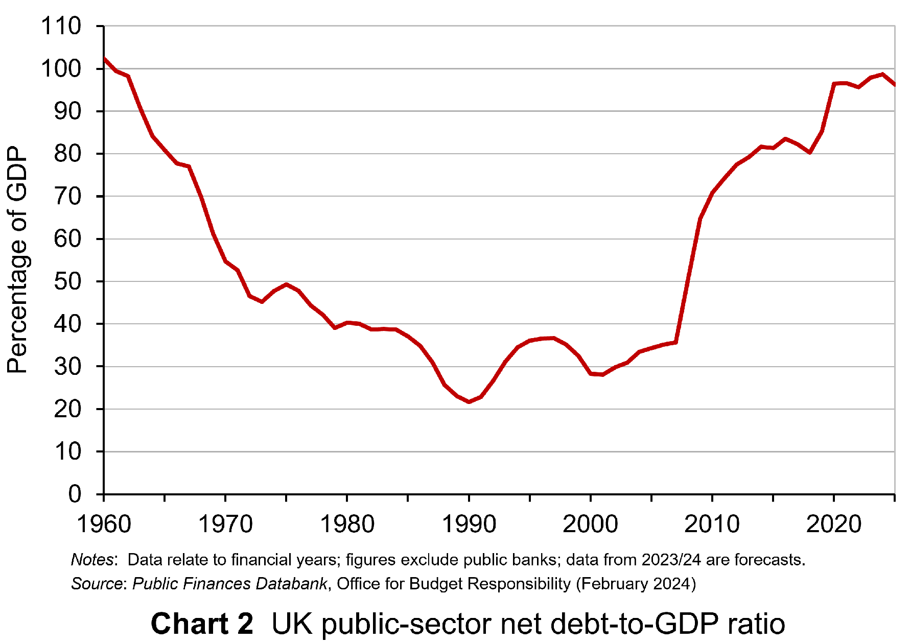 The second topic area that I have been discussing in my final-year macroeconomics classes has centred around fiscal policy and the state of the public finances. The context for this is that we have seen a significant increase in public debt-to-GDP ratios over the past couple of decades as the public sector has attempted to absorb significant economic shocks. These include the global financial crisis of 2007–8, the COVID-19 pandemic and the cost-of-living crisis. These interventions in the case of the UK have seen its public debt-to-GDP ratio more than triple since the early 2000s to close to 100% (see Chart 2: click here for a PowerPoint).
Understandably, given the stresses placed on the public finances, economists have increasingly debated issues around debt sustainability. These debates have been mirrored by politicians and policymakers. A key question is whether to have a public debt rule. The UK has in recent years adopted such a rule. The arguments for a rule centre on ensuring sound public finances and maintaining the confidence of investors to purchases public debt. A debt rule therefore places a discipline on fiscal policy, with implications for taxation and spending.
How easy it is to stick to a debt rule depends on three key factors. It will be harder to stick to the rule:
- The higher the current debt-to-GDP ratio and hence the more it needs to be reduced to meet the rule.
- The higher the rate of interest and hence the greater the cost of servicing the public debt.
- The lower the rate of economic growth and hence the less quickly will tax revenues rise.
With a given debt-to-GDP ratio, a given average interest rate payable on its debt, and a given rate of economic growth, we can determine the primary fiscal balance relative to GDP a government would need to meet for the debt-to-GDP ratio to remain stable. This is known as the ‘debt-stabilising primary balance’. The primary balance is the difference between a government’s receipts and its expenditures less the interest payments on its debt.
 This fiscal arithmetic is important in determining a government’s fiscal choices. It shows the implications for spending and taxation. These implications become ever more important and impactful on people, businesses, and society when the fiscal arithmetic becomes less favourable. This is a situation that appears to be increasingly the case for many countries, including the UK, as the rate of interest on public debt rises relative to a country’s rate of economic growth. As this happens, governments are increasingly required to run healthier primary balances. This of course implies a tightening of their fiscal stance.
Hence, the fiscal conversations with my students have focused on both the benefits and the costs of debt-stabilisation. In respect of the costs, a few issues have arisen.
First, as with the inflation-rate target, it is hard to identify an optimal public debt-to-GDP ratio number. While the fiscal arithmetic may offer some clue, it is not straightforward to address the question as to whether a debt-to-GDP ratio of say 100% or 120% would be excessive for the UK.
Second, it is possible that the debt stabilisation itself can make the fiscal arithmetic of debt stabilisation more difficult. This occurs if fiscal consolidation itself hinders long-term economic growth, which then makes the fiscal arithmetic more difficult. This again points to the difficulties in designing policy frameworks, whether they be for monetary or fiscal policy.
Third, a focus on debt stabilisation alone ignores the fact that there are two sides to any sector’s balance sheet. It would be very unusual when assessing the well-being of businesses or households if we were to ignore the asset side of their balance sheet. Yet, this is precisely the danger of focusing on public debt at the exclusion of what fiscal choices can mean for public-sector assets, from which we all can potentially benefit. Hence, some would suggest a more balanced approach to assessing the soundness of the public finances might involve a net worth (assets less liabilities) measure. This has parallels with the debates around whether mandates of central banks should be broader.
Applications in macroeconomics
What my teaching of a topics-based macroeconomics module this term has vividly demonstrated is that concepts, theories, and models come alive, and are capable of being understood better, when they are used to shine a light on real-world issues. The light being shone on monetary and fiscal policy in today’s turbulent macroeconomic environment is perhaps understandably very bright.
Indeed, the light being shone on fiscal policy in the UK and some other countries facing an upcoming election, is intensified further with the state of the public finances shaping much of the public discourse on fiscal choices. Hopefully, my students will continue to debate these important issues beyond their graduation, stressing their importance for people’s lives and, in doing so, going beyond the abstract.
References
- Rules rather than discretion: The inconsistency of optimal plans
The Journal of Political Economy, Finn E Kydland and Edward C. Prescott (1977, 85(3), pp 473–92) - The optimal degree of commitment to an intermediate monetary target
Quarterly Journal of Economics, Kenneth Rogoff (November 1985, 100(4), pp 1169–89) - Discretion versus policy rules in practice
Carnegie-Rochester Conference Series on Public Policy, John B Taylor (December 1993, 39, pp 195–214)
Articles
- If markets are right about long real rates, public debt ratios will increase for some time. We must make sure that they do not explode.
- Changing the rules of the game: a fiscal framework for fair growth
- The case for rethinking fiscal rules is overwhelming
- Controlling debt is just a means — it is not a government’s end
- The damning truth about the UK’s 2% inflation target: it’s completely made up
- What are the UK’s ‘fiscal rules’ and why is the OBR under attack?
Peterson Institute for International Economics, Olivier Blanchard (6/11/23)
Inclusive growth in action, The Centre for Progressive Policy, Rosie Fogden (23/7/23)
Financial Times, Andy Haldane (16/5/23)
Financial Times, Martin Wolf (13/11/23)
The Guardian, Louis-Philippe Rochon (1/2/24)
The Guardian, Richard Partington (5/3/24)
Questions
- What is meant by time-inconsistent monetary policy announcements? How has this concept been important for the way in which many central banks now conduct monetary policy?
- What is meant by a ‘conservative’ central banker? Why is the appointment of this type of central banker thought to be important in affecting inflation?
- What is the contemporary macroeconomic relevance of the inflation–output (or inflation–unemployment) stabilisation trade-off?
- How is the primary balance different from the actual budget balance?
- What do you understand by the concept of ‘the fiscal arithmetic’. Explain how each element of the fiscal arithmetic affects the debt-stabilising primary balance?
- Analyse the costs of benefits of a debt-based fiscal rule.
 The past decade or so has seen large-scale economic turbulence. As we saw in the blog
 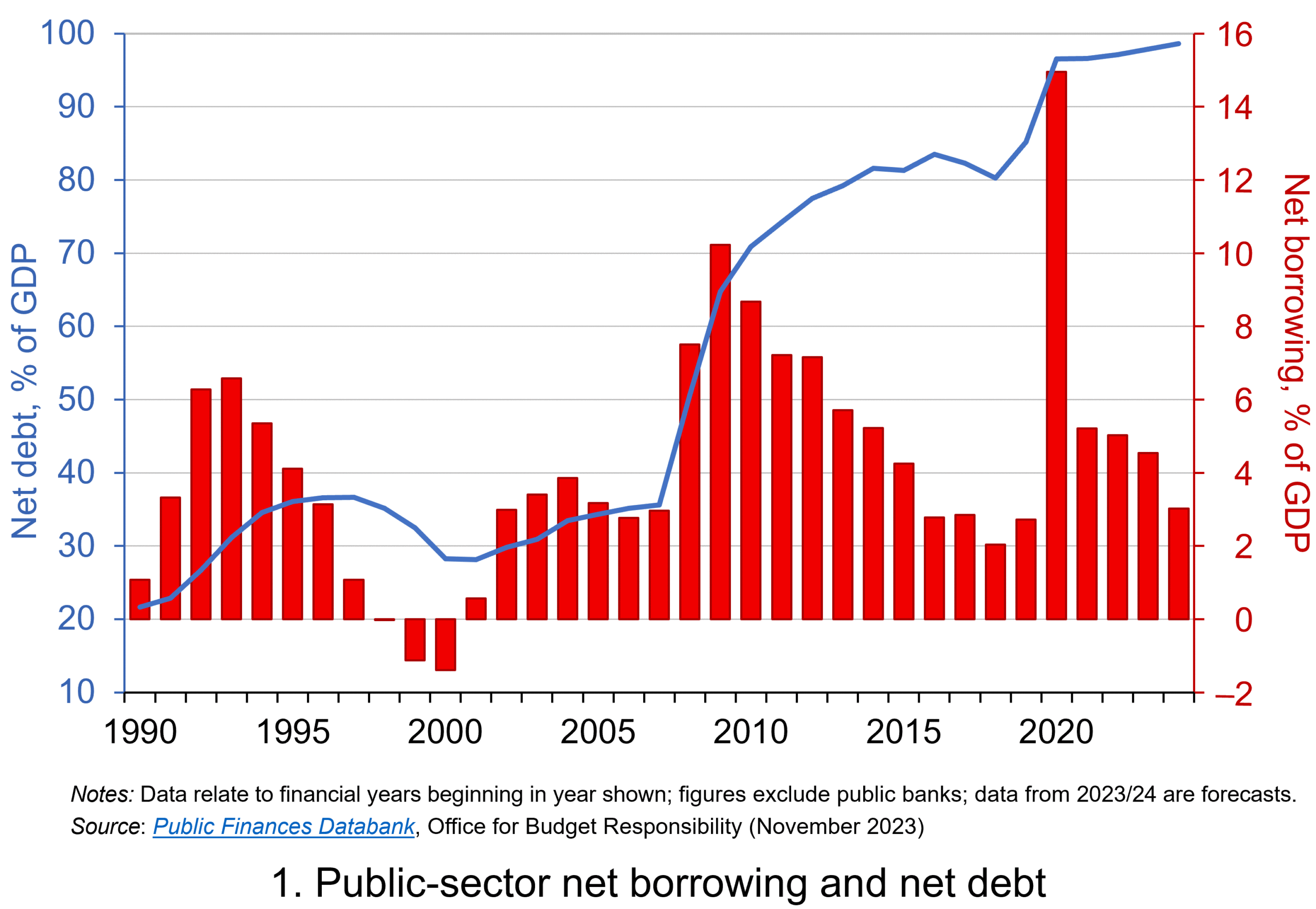 Chart 1 shows the path of UK public-sector net debt and net borrowing, as percentages of GDP, since 1990. Debt is a stock concept and is the result of accumulated flows of past borrowing. Net debt is simply gross debt less liquid financial assets, which mainly consist of foreign exchange reserves and cash deposits. Net borrowing is the headline measure of the sector’s deficit and is based on when expenditures and receipts (largely taxation) are recorded rather than when cash is actually paid or received. (Click
  The ratcheting up of debt levels affects debt servicing costs and hence the budgetary position of government. Yet the recent increases in interest rates also raise the costs faced by governments in financing future deficits or refinancing existing debts that are due to mature. In addition, a continuation of the low economic growth that has beset the UK economy since the global financial crisis also has implications for the burden imposed on the public sector by its debts, and hence the sustainability of the public finances. After all, low growth has implications for spending commitments, and, of course, the flow of receipts.
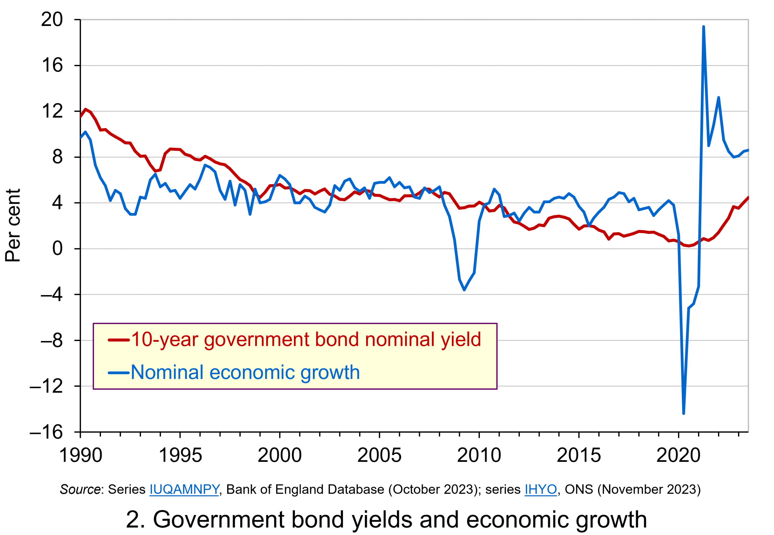 Consider Charts 2 and 3 to understand how the ‘r – g’ differential has affected debt sustainability in the UK since 1990. Chart 2 plots the implied yield on 10-year government bonds, alongside the annual rate of nominal growth (click
 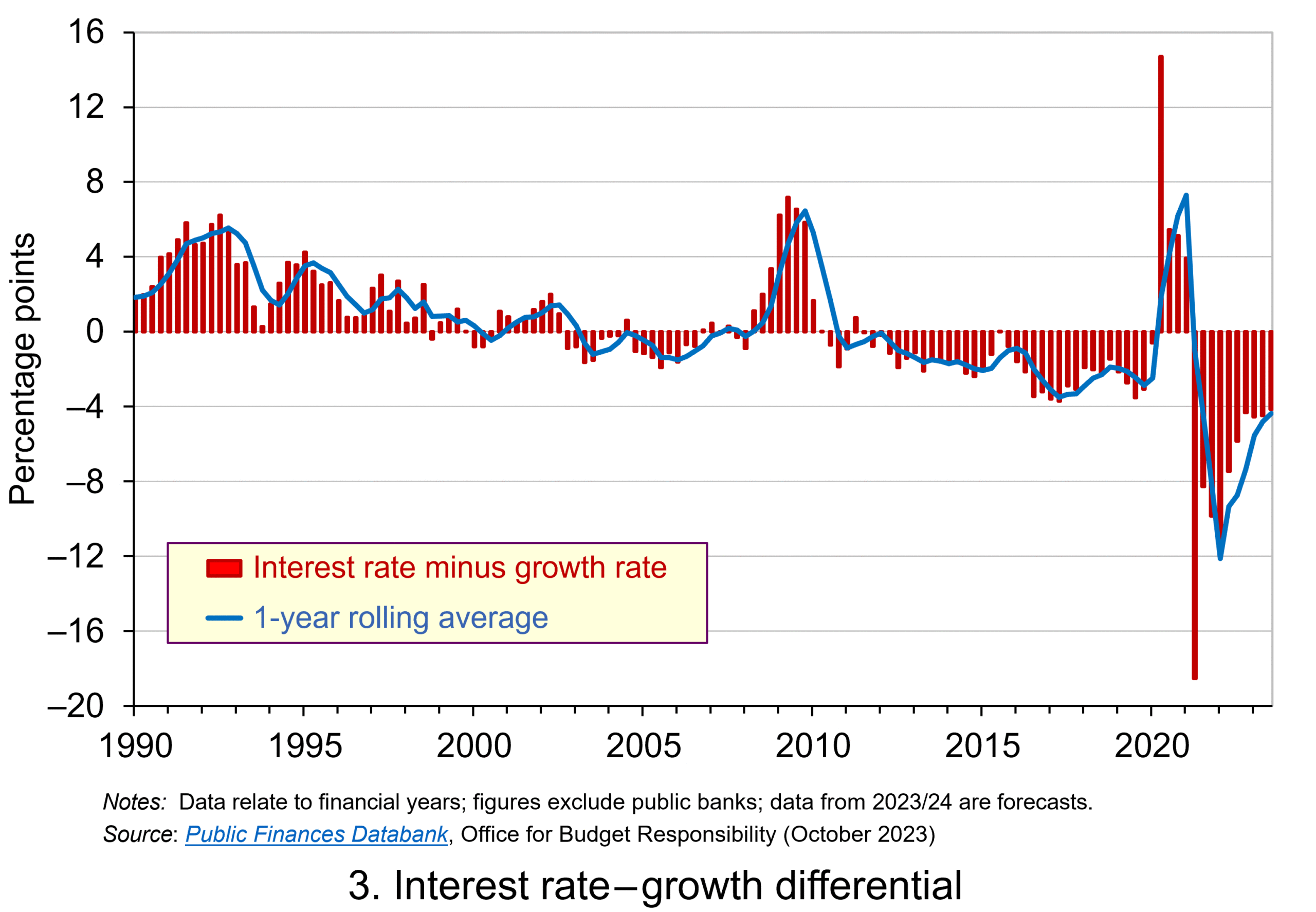 Chart 3 plots the ‘r – g’ differential which is simply the difference between the two series in Chart 2, along with a 12-month rolling average of the differential to help show better the direction of the differential by smoothing out some of the short-term volatility (click
 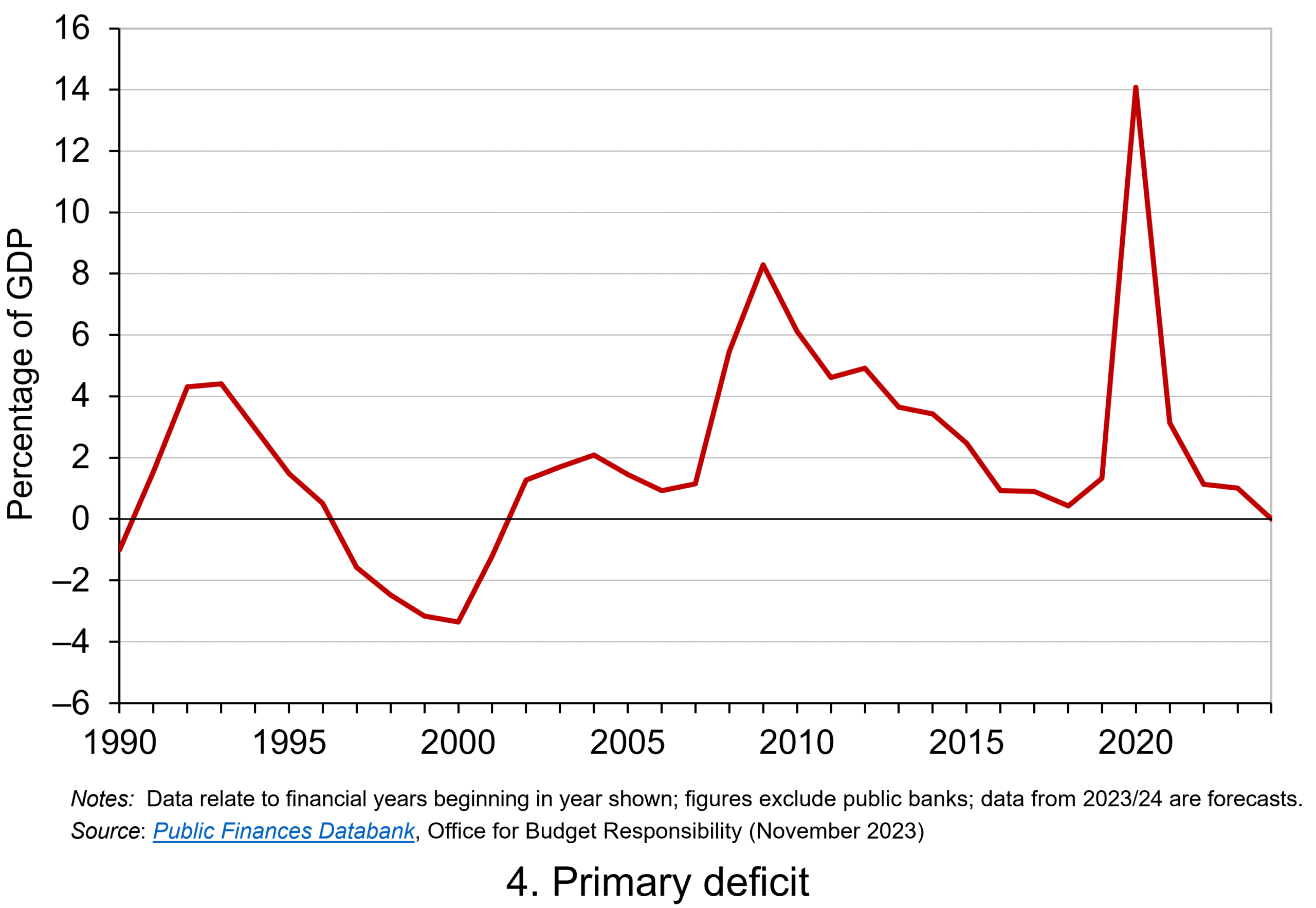 Yet the negative differential resumed in 2010 and continued up to the pandemic. Again, this is indicative of the macroeconomic and financial environments being supportive of the public finances. It was, however, largely driven by low interest rates rather than by economic growth.
  The pandemic saw the ‘r – g’ differential again turn markedly positive, averaging 7 percentage points in the four quarters from Q2 of 2020. While the differential again turned negative, the debt-to-GDP ratio had also increased substantially because of large-scale fiscal interventions. This made the negative differential even more important for the sustainability of the public finances. The question is how long the negative differential can last.