 To finance budget deficits, governments have to borrow. They can borrow short-term by issuing Treasury bills, typically for 1, 3 or 6 months. These do not earn interest and hence are sold at a discount below the face value. The rate of discount depends on supply and demand and will reflect short-term market rates of interest. Alternatively, governments can borrow long-term by issuing bonds. In the UK, these government securities are known as ‘gilts’ or ‘gilt-edged securities’. In the USA they are known as ‘treasury bonds’, ‘T-bonds’ or simply ‘treasuries’. In the EU, countries separately issue bonds but the European Commission also issues bonds.
In the UK, gilts are issued by the Debt Management Office on behalf of the Treasury. Although there are index-linked gilts, the largest proportion of gilts are conventional gilts. These pay a fixed sum of money per annum per £100 of face value. This is known as the ‘coupon payment’ and the rate is set at the time of issue. The ‘coupon rate’ is the payment per annum as a percentage of the bond’s face value:

Payments are made six-monthly. Each issue also has a maturity date, at which point the bonds will be redeemed at face value. For example, a 4½% Treasury Gilt 2028 bond has a coupon rate of 4½% and thus pays £4.50 per annum (£2.25 every six months) for each £100 of face value. The issue will be redeemed in June 2028 at face value. The issue was made in June 2023 and thus represented a 5-year bond. Gilts are issued for varying lengths of time from 2 to 55 years. At present, there are 61 different conventional issues of bonds, with maturity dates varying from January 2024 to October 2073.
Bond prices
 Bonds can be sold on the secondary market (i.e. the stock market) before maturity. The market price, however, is unlikely to be the coupon price (i.e. the face value). The lower the coupon rate relative to current interest rates, the less valuable the bond will be. For example, if interest rates rise, and hence new bonds pay a higher coupon rate, the market price of existing bonds paying a lower coupon rate must fall. Thus bond prices vary inversely with interest rates.
The market price also depends on how close the bonds are to maturity. The closer the maturity date, the closer the market price of the bond will be to the face value.
Bond yields: current yield
A bond’s yield is the percentage return that a person buying the bond receives. If a newly issued bond is bought at the coupon price, its yield is the coupon rate.
However, if an existing bond is bought on the secondary market (the stock market), the yield must reflect the coupon payments relative to the purchase price, not the coupon price. We can distinguish between the ‘current yield’ and the ‘yield to maturity’.
The current yield is the coupon payment as a percentage of the current market price of the bond:

Assume a bond were originally issued at 2% (its coupon rate) and thus pays £2 per annum. In the meantime, however, assume that interest rates have risen and new bonds now have a coupon rate of 4%, paying £4 per annum for each £100 invested. To persuade people to buy old bonds with a coupon rate of 2%, their market prices must fall below their face value (their coupon price). If their price halved, then they would pay £2 for every £50 of their market price and hence their current yield would be 4% (£2/£50 × 100).
Bond yields: yield to maturity (YTM)
But the current yield does not give the true yield – it is only an approximation. The true yield must take into account not just the market price but also the maturity value and the length of time to maturity (and the frequency of payments too, which we will ignore here). The closer a bond is to its maturity date, the higher/lower will be the true yield if the price is below/above the coupon price: in other words, the closer will the market price be to the coupon price for any given market rate of interest.
A more accurate measure of a bond’s yield is thus the ‘yield to maturity’ (YTM). This is the interest rate which makes the present value of all a bond’s future cash flows equal to its current price. These cash flows include all coupon payments and the payment of the face value on maturity. But future cash flows must be discounted to take into account the fact that money received in the future is worth less than money received now, since money received now could then earn interest.
The yield to maturity is the internal rate of return (IRR) of the bond. This is the discount rate which makes the present value (PV) of all the bond’s future cash flows (including the maturity payment of the coupon price) equal to its current market price. For simplicity, we assume that coupon payments are made annually. The formula is the one where the bond’s current market price is given by:

Where: t is the year; n is the number of years to maturity; YTM is the yield to maturity.
Thus if a bond paid £5 each year and had a maturity value of £100 and if current interest rates were higher than 5%, giving a yield to maturity of 8%, then the bond price would be:

In other words, with a coupon rate of 5% and a higher YTM of 8%, the bond with a face value of £100 and five years to maturity would be worth only £88.02 today.
If you know the market price of a given bond, you can work out its YTM by substituting in the above formula. The following table gives examples.
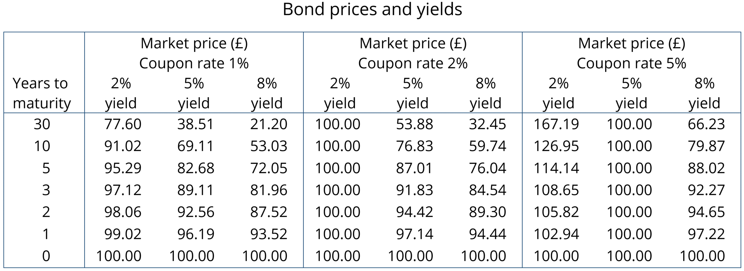
The higher the YTM, the lower the market price of a bond. Since the YTM reflects in part current rates of interest, so the higher the rate of interest, the lower the market price of any given bond. Thus bond yields vary directly with interest rates and bond prices vary inversely. You can see this clearly from the table. You can also see that market bond prices converge on the face value as the maturity date approaches.
Recent activity in bond markets
Investing in government bonds is regarded as very safe. Coupon payments are guaranteed, as is repayment of the face value on the maturity date. For this reason, many pension funds hold a lot of government bonds issued by financially trustworthy governments. But in recent months, bond prices in the secondary market have fallen substantially as interest rates have risen. For those holding existing bonds, this means that their value has fallen. For governments wishing to borrow by issuing new bonds, the cost has risen as they have to offer a higher coupon rate to attract buyers. This make it more expensive to finance government debt.
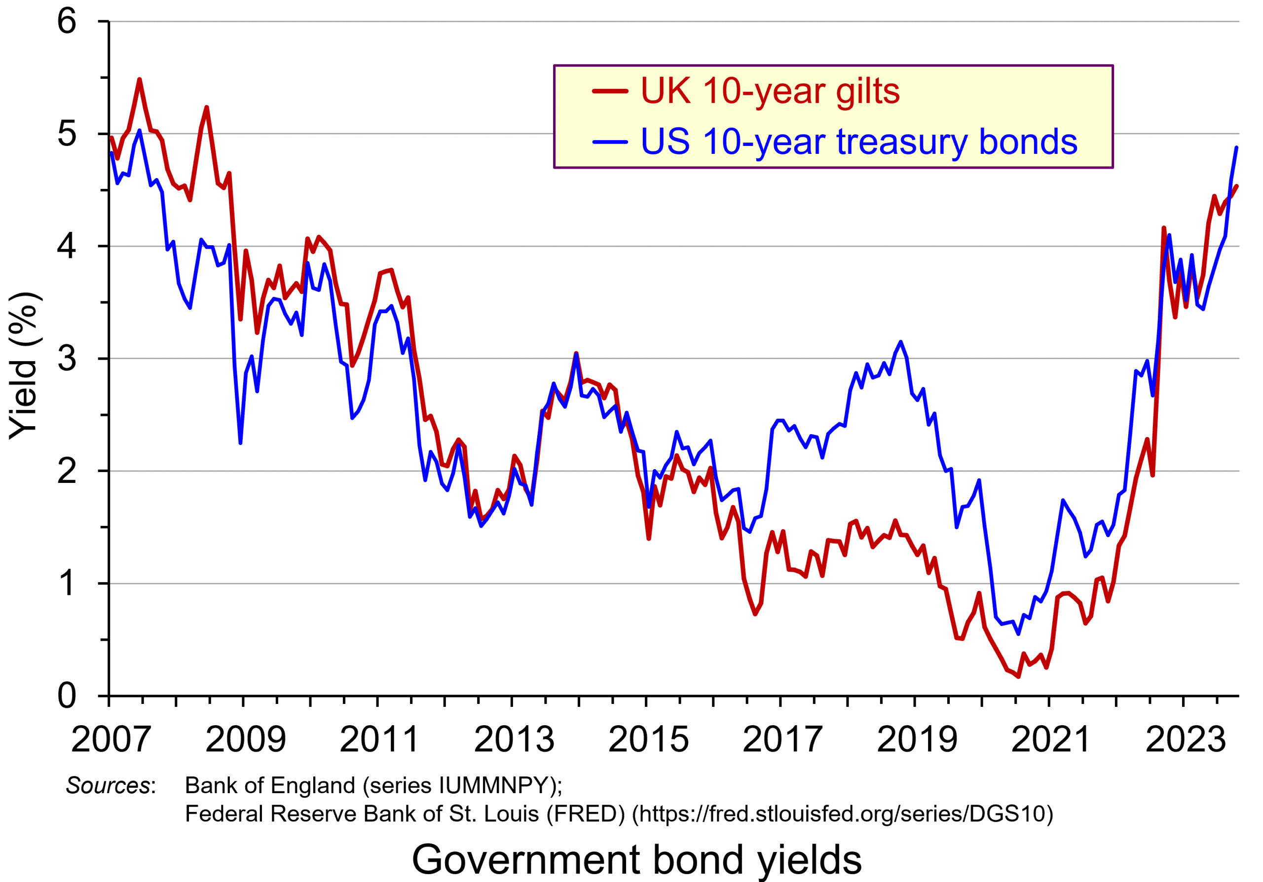 The chart shows the yield on 10-year government bonds. It is calculated using the ‘par value’ approach. This gives the coupon rate that would have to be paid for the market price of a bond to equal its face value. Clearly, as interest rates rise, a bond would have to pay a higher coupon rate for this to happen. (This, of course, is only hypothetical to give an estimate of market rates, as coupon rates are fixed at the time of a bond’s issue.)
Par values reflect both yield to maturity and also expectations of future interest rates. The higher people expect future interest rates to be, the higher must par values be to reflect this.
 In the years following the financial crisis of 2007–8 and the subsequent recession, and again during the COVID pandemic, central banks cut interest rates and supported this by quantitative easing. This involved central banks buying existing bonds on the secondary market and paying for them with newly created (electronic) money. This drove up bond prices and drove down yields (as the chart shows). This helped support the policy of low interest rates. This was a boon to governments, which were able to borrow cheaply.
This has all changed. With quantitative tightening replacing quantitative easing, central banks have been engaging in asset sales, thereby driving down bond prices and driving up yields. Again, this can be seen in the chart. This has helped to support a policy of higher interest rates.
Problems of higher bond yields/lower bond prices
Although lower bond prices and higher yields have supported a tighter monetary policy, which has been used to fight inflation, this has created problems.
First, it has increased the cost of financing government debt. In 2007/8, UK public-sector net debt was £567bn (35.6% of GDP). The Office for Budget Responsibility forecasts that it will be £2702bn (103.1% of GDP in the current financial year – 2023/24). Not only, therefore, are coupon rates higher for new government borrowing, but the level of borrowing is now a much higher proportion of GDP. In 2020/21, central government debt interest payments were 1.2% of GDP; by 2022/23, they were 4.4% (excluding interest on gilts held in the Bank of England, under the Asset Purchase Facility (quantitative easing)).
 In the USA, there have been similar increases in government debt and debt interest payments. Debt has increased from $9tn in 2007 to $33.6tn today. Again, with higher interest rates, debt interest as a percentage of GDP has risen: from 1.5% of GDP in 2021 to a forecast 2.5% in 2023 and 3% in 2024. What is more, 31 per cent of US government bonds will mature next year and will need refinancing – at higher coupon rates.
There is a similar picture in other developed countries. Clearly, higher interest payments leave less government revenue for other purposes, such as health and education.
Second, many pension funds, banks and other investment companies hold large quantities of bonds. As their price falls, so this reduces the value of these companies’ assets and makes it harder to finance new purchases, or payments or loans to customers. However, the fact that new bonds pay higher interest rates means that when existing bond holdings mature, the money can be reinvested at higher rates.
Third, bonds are often used by companies as collateral against which to borrow and invest in new capital. As bond prices fall, this can hamper companies’ ability to invest, which will lead to lower economic growth.
Fourth, higher bond yields divert demand away from equities (shares). With equity markets falling back or at best ceasing to rise, this erodes the value of savings in equities and may make it harder for firms to finance investment through new issues.
At the core of all these problems is inflation and budget deficits. Central banks have responded by raising interest rates. This drives up bond yields and drives down bond prices. But bond prices and yields depend not just on current interest rates, but also on expectations about future interest rates. Expectations currently are that budget deficits will be slow to fall as governments seek to support their economies post-COVID. Also expectations are that inflation, even though it is falling, is not falling as fast as originally expected – a problem that could be exacerbated if global tensions increase as a result of the ongoing war in Ukraine, the Israel/Gaza war and possible increased tensions with China concerning disputes in the China Sea and over Taiwan. Greater risks drive up bond yields as investors demand a higher interest premium.
Articles
Information and data
Questions
- Why do bond prices and bond yields vary inversely?
- How are bond yields and prices affected by expectations?
- Why are ‘current yield’ and ‘yield to maturity’ different?
- What is likely to happen to bond prices and yields in the coming months? Explain your reasoning.
- What constraints do bond markets place on fiscal policy?
- Would it be desirable for central banks to pause their policy of quantitative tightening?
 In her bid to become Conservative party leader, Liz Truss promised to make achieving faster economic growth her number-one policy objective. This would involve pursuing market-orientated supply-side policies.
These policies would include lower taxes on individuals to encourage people to work harder and more efficiently, and lower taxes on business to encourage investment. The policy would also involve deregulation, which would again encourage investment, both domestic and inward investment from overseas. These proposals echoed the policies pursued in the 1980s by President Ronald Reagan in the USA and Margaret Thatcher in the UK.
On September 23, the new Chancellor, Kwasi Kwarteng, presented a ‘mini-Budget’ – although the size of the changes made it far from ‘mini’. This, as anticipated, included policies intended to boost growth, including scrapping the 45% top rate of income tax, which is currently paid by people earning over £150 000 (a policy withdrawn on 3 October after massive objections), cutting the basic rate of income tax from 20% to 19%, scrapping the planned rise in corporation tax from 19% to 25%, scrapping the planned rise in national insurance by 1.25 percentage points, a cut in the stamp duty on house purchase and scrapping the limit placed on bankers’ bonuses. In addition, he announced the introduction of an unlimited number of ‘investment zones’ which would have lower business taxes, streamlined planning rules and lower regulation. The policies would be funded largely from extra government borrowing.
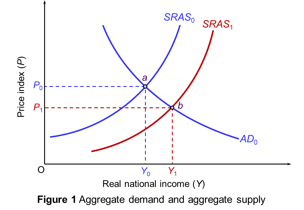 Theoretically, the argument is simple. If people do work harder and firms do invest more, then potential GDP will rise – a rise in aggregate supply. This can be shown on an aggregate demand and supply diagram. If the policy works, the aggregate supply curve will shift to the right. Real GDP will rise and there will be downward pressure on prices. In Figure 1, real GDP will rise from Y0 to Y1 and the price level will fall from P0 to P1. However, things are not as simple as this. Indeed, there are two major problems.
The first concerns whether tax cuts will incentivise people to work harder. The second concerns what happens to aggregate demand. I addition to this, the policies are likely to have a profound effect on income distribution.
Tax cuts and incentives
Cutting the top rate of income tax would have immediately given people at the top of the income scale a rise in post-tax income. This would have created a substitution effect and an income effect. Each extra pound that such people earn would be worth more in post-tax income – 60p rather than 55p. This would provide an incentive for people to substitute work for leisure as work is now more rewarding. This is the substitution effect. On the other hand, with the windfall of extra income, they now would have needed to work less in order to maintain their post-tax income at its previous level. They may well indeed, therefore, have decided to work less and enjoy more leisure. This is the income effect.
With the diminishing marginal utility of income, generally the richer people are, the bigger will be the income effect and the smaller the substitution effect. Thus, cutting the top rate of income tax may well have led to richer people working less. There is no evidence that the substitution effect would be bigger.
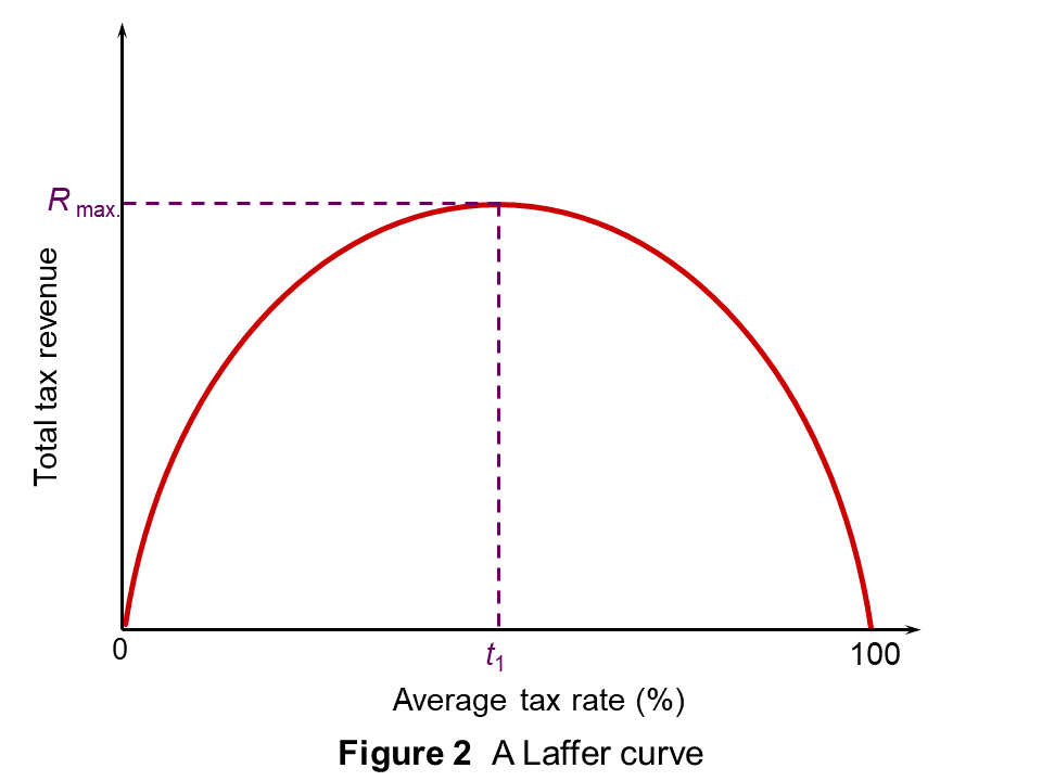 If top rates of income tax are already at a very high level, then cutting then may well encourage more work. After all, there is little incentive to work more if the current rate of tax is over 90%, say. Cutting them to 80% could have a big effect. This was the point made by Art Laffer, one of Ronald Reagan’s advisors. He presented his arguments in terms of the now famous ‘Laffer curve’, shown in Figure 2. This shows the total tax revenue raised at different tax rates.
If the average tax rate were zero, no revenue would be raised. As the tax rate is raised above zero, tax revenues will increase. The curve will be upward sloping. Eventually, however, the curve will peak (at tax rate t1). Thereafter, tax rates become so high that the resulting fall in output more than offsets the rise in tax rate. When the tax rate reaches 100 per cent, the revenue will once more fall to zero, since no one will bother to work.
If the economy were currently to the right of t1, then cutting taxes would increase revenue as there would be a major substitution effect. However, most commentators argue that the UK economy is to the left of t1 and that cutting the top rate would reduce tax revenues. Analysis by the Office for Budget Responsibility in 2012 suggested that t1 for the top rate of income tax was at around 48% and that cutting the rate below that would reduce tax revenue. Clearly according to this analysis, 40% is considerably below t1.
As far as corporation tax is concerned, the 19% rate is the lowest in the G20 and yet the UK suffers from low rates of both domestic investment and inward direct investment. There is no evidence that raising it somewhat, as previously planned, will cut investment. And as far as individual entrepreneurs are concerned, cutting taxes is likely to have little effect on the desire to invest and expand businesses. The motivation of entrepreneurs is only partly to do with the money. A major motivation is the sense of achievement in building a successful business.
Creating investment zones with lower taxes, no business rates and lower regulations may encourage firms to set up there. But much of this could simply be diverted investment from elsewhere in the country, leaving overall investment little changed.
To assess these questions, the government needs to model the outcomes and draw on evidence from elsewhere. So far this does not seem to have happened. They government did not even present a forecast of the effects of its policies on the public finances, something that the OBR normally presents at Budget time. This was one of the reasons for the collapse in confidence of sterling and gilts (government bonds) in the days following the mini-Budget.
Effects on aggregate demand
 Cutting taxes and financing them from borrowing will expand aggregate demand. In Figure 1, the AD curve will also shift to the right and this will push up prices. Inflation is already a serious problem in the economy and unfunded tax cuts will make it worse. Higher inflation will result in the Bank of England raising interest rates further to curb aggregate demand. But higher interest rates, by raising borrowing costs, are likely to reduce investment, which will have a negative supply-side effect.
The problem here is one of timing. Market-orientated supply-side policies, if they work to increase potential GDP, will take time – measured in years rather than months. The rise in aggregate demand will be much quicker and will thus precede the rise in supply. This could therefore effectively kill off the rise in supply as interest rates rise, the exchange rate falls and the economy is pushed towards recession. Indeed, the mini-Budget immediately sparked a run on the pound and the exchange rate fell.
The rising government debt may force the government to make cuts in public expenditure. Rather than cutting current expenditure on things such as nurses, teachers and benefits, it is easier to cut capital expenditure on things such as roads and other infrastructure. But this will have adverse supply-side effects.
Effects on income distribution
 Those advocating market-orientated supply-side policies argue that, by making GDP bigger, everyone can gain. They prefer to focus on the size of the national ‘pie’ rather than its distribution. If the rich initially gain, the benefits will trickle down to the poorest in society. This trickle-down theory was popular in the 1980s with politicians such as Margaret Thatcher and Ronald Reagan and, more recently, with Republican presidents, such as Goerge W Bush and Donald Trump. There are two problems with this, however.
The first, which we have already seen, is whether such policies actually do increase the size of the ‘pie’.
The second is how much does trickle down. During the Thatcher years, income inequality in the UK grew, as it did in the USA under Ronald Reagan. According to an IMF study in 2015 (see the link to the IMF analysis below), policies that increase the income share of the poor and the middle class do increase growth, while those that raise the income share of the top 20 per cent result in lower growth.
After the mini-Budget was presented, the IMF criticised it for giving large untargeted tax cuts that would heighten inequality. The poor would gain little from the tax cuts. The changes to income tax and national insurance mean that someone earning £20 000 per year will gain just £167 per year, while someone earning £200 000 will gain £5220. What is more, the higher interest rates and higher prices resulting from the lower exchange rate are likely to wipe out the modest gains to the poor.
Podcast
Articles
- At a glance: What’s in the mini-budget?
BBC News (23/9/22)
- Mini-budget: What it means for you and your finances
BBC News, Kevin Peachey (23/8/22)
- Will this huge tax cutting gamble pay off?
BBC News, Faisal Islam (23/9/22)
- Kwasi Kwarteng faces U-turn on tax or spending cuts
BBC News, Faisal Islam (28/9/22)
- Nearly 300 UK mortgage deals pulled in a day as pound’s fall heralds rate rise
The Guardian, Zoe Wood (27/9/23)
- Rationale behind abolition of 45p tax rate reflects failed ideology
The Guardian, Arun Advani, David Burgherr and Andy Summers (29/9/23)
- The UK’s ‘Trussonomics’ crashes the pound and leaves investors shaking their heads
CNN, Allison Morrow (26/9/23)
- Mini budget: will Kwasi Kwarteng’s plan deliver growth?
The Conversation, Steve Schifferes (23/9/23)
- Only a U-turn by the government or the Bank of England will calm UK financial markets
The Conversation, Campbell Leith (28/9/22)
- IMF gives damning verdict on Britain’s tax cuts
CNBC, Hannah Ward-Glenton (28/9/23)
- Lasting effects of ‘mini’ Budget will be felt far beyond the trading floors
Today News, Torsten Bell (1/10/23)
Analysis
- Causes and Consequences of Income Inequality: A Global Perspective
IMF Staff Discussion Notes, Era Dabla-Norris, Kalpana Kochhar, Nujin Suphaphiphat, Franto Ricka and Evridiki Tsounta (15/6/15)
- Mini-Budget response
Institute for Fiscal Studies, Stuart Adam, Isaac Delestre, Carl Emmerson, Paul Johnson, Robert Joyce, Isabel Stockton, Tom Waters, Xiaowei Xu and Ben Zaranko (23/9/22)
Questions
- Distinguish between market-orientated supply-side policies and interventionist ones. Consider the advantages and disadvantages of each.
- Explain why bond prices fell after the mini-Budget. What was the Bank of England’s response and why did this run counter to its plan for quantitative tightening?
- How might a tax-cutting Budget be designed to help the poor rather than the rich? Would this have beneficial supply-side effects?
- Find out about the 1972 tax-cutting Budget of Anthony Barber, the Chancellor in Ted Heath’s government, that led to the ‘Barber boom’ and then rampant inflation. Are there any similarities between the 1972 Budget and the recent mini-Budget?
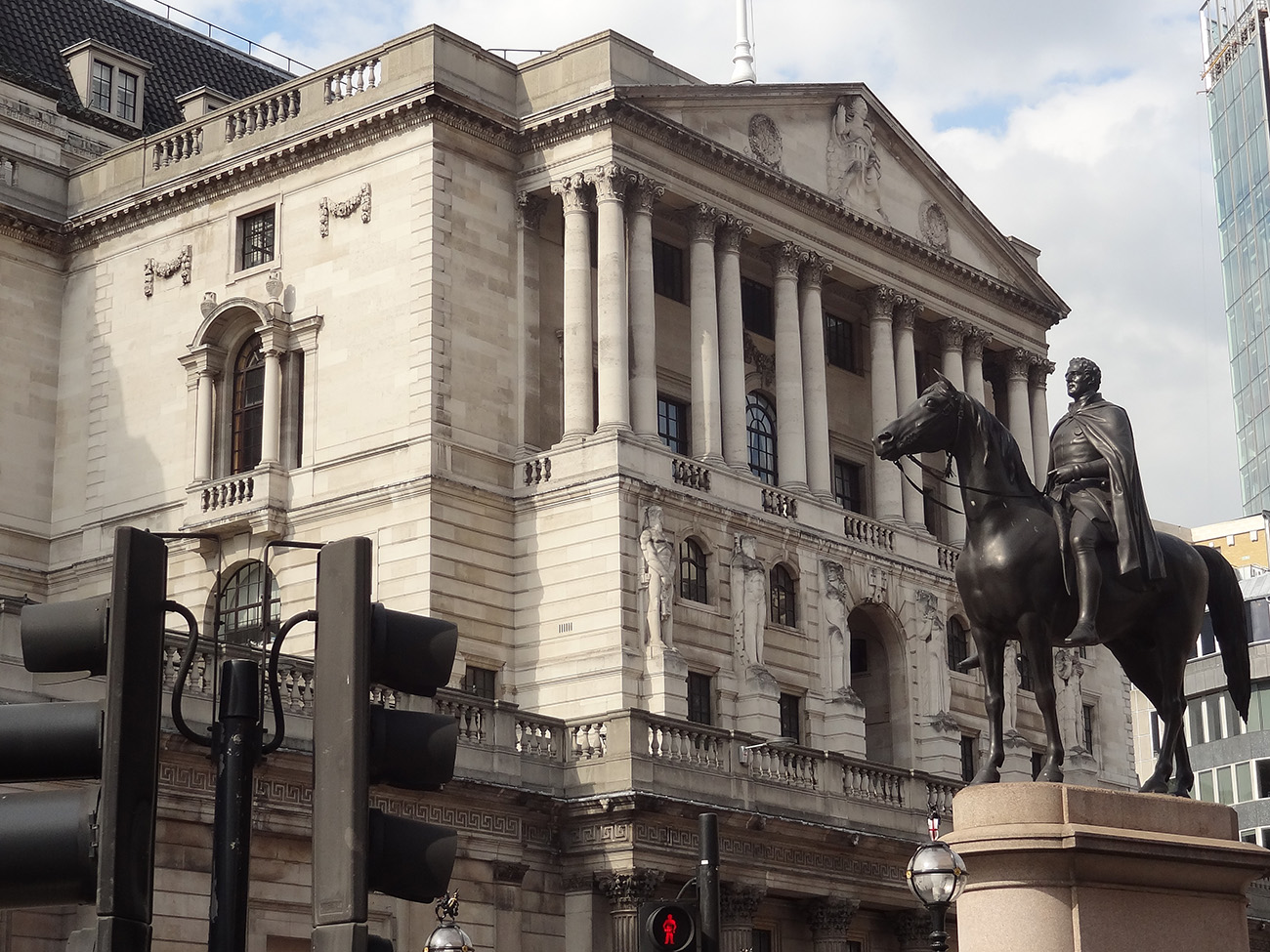 At its meeting on 6 May, the Bank of England’s Monetary Policy Committee decided to keep Bank Rate at 0.1%. Due to the significant impact of COVID-19 and the measures put in place to try to contain the virus, the MPC voted unanimously to keep Bank Rate the same.
However, it decided not to launch a new stimulus programme, with the committee voting by a majority of 7-2 for the Bank to continue with the current programme of quantitative easing. This involves the purchase of £200 billion of government and sterling non-financial investment-grade corporate bonds, bringing the total stock of bonds held by the Bank to £645 billion.
The Bank forecast that the crisis will put the economy into its deepest recession in 300 years, with output plunging 30 per cent in the first half of the year.
Monetary policy and MPC
Monetary policy is the tool used by the UK’s central bank to influence how much money is in the economy and how much it costs to borrow. The Bank of England’s main monetary policy tools include setting the Bank Rate and quantitative easing (QE). Bank Rate is the interest rate charged to banks when they borrow money from the BoE. QE is the process of creating money digitally to buy corporate and government bonds.
The BoE’s Monetary Policy Committee (MPC) sets monetary policy to meet the 2% inflation target. Maintaining a low and stable inflation rate is good for the economy and it is the main monetary policy aim. However, the Bank also has to balance this target with the government’s other economic aims of sustaining growth and employment in the economy.
Actions taken by the MPC
It is challenging to respond to severe economic and financial disruption, with the UK economy looking unusually uncertain. Activity has fallen sharply since the beginning of the year and unemployment has risen markedly. The current rate of inflation, measured by the Consumer Price Index (CPI), declined to 1.5% in March and is likely to fall below 1% in the next few months. Household consumption has fallen by around 30% as consumer confidence has declined. Companies’ sales are expected to be around 45% lower than normal and business investment 50% lower.
In the current circumstances, and consistent with the MPC’s remit, monetary policy is aimed at supporting businesses and households through the crisis and limiting any lasting damage to the economy. The Bank has used both main monetary tools to fulfil its mandate and attempt to boost the economy amid the current lockdown. The Bank Rate was reduced to 0.1% in March, the lowest level in the Bank’s 325-year history and the current programme of QE was introduced in March.
What is next?
This extraordinary time has seen the outlook for the all global economies become uncertain.  The long-term outcome will depend critically on the evolution of the pandemic, and how governments, households and businesses respond to it. The Bank of England has stated that businesses and households will need to borrow to get through this period and is encouraging banks and building societies to increase their lending. Britain’s banks are warned that if they try to stem losses by restricting lending, they will make the situation worse. The Bank believes that the banks are strong enough to keep lending, which will support the economy and limit losses to themselves.
In the short term, a bleak picture of the UK economy is suggested, with a halving in business investment, a near halving in business sales, a sharp rise in unemployment and households cutting their spending by a third. Despite its forecast that GDP could shrink by 14% for 2020, the Bank of England is forecasting a ‘V’ shaped recovery. In this scenario, the recovery in economic activity, once measures are softened, is predicted to be relatively rapid and inflation rises to around the 2 per cent target. However, this would be after a dip to 0.5% in 2021, before returning to the 2 per cent target the following year.
However, there are some suggestions that the Bank’s forecast for the long-term recovery is too optimistic. Yael Selfin, chief economist at KPMG UK, fears the UK economy could shrink even more sharply than the Bank of England has forecast.
Despite the stark numbers issued by the Bank of England today, additional pressure on the economy is likely. Some social distancing measures are likely to remain in place until we have a vaccine or an effective treatment for the virus, with people also remaining reluctant to socialise and spend. That means recovery is unlikely to start in earnest before sometime next year.
 There are also additional factors that could dampen future productivity, such as the impact on supply chains, with ‘just-in-time’ operations potentially being a thing of the past.
There is also the ongoing issue of Brexit. This is a significant downside risk as the probability of a smooth transition to a comprehensive free-trade agreement with the EU in January is relatively small. This will only increase uncertainty for businesses along with the prospect of increased trade frictions next year.
Conclusion
The predictions from the Bank of England are based on many assumptions, one of which is that the economy will only be gradually released from lockdown. Its numbers contain the expectations that consumer and worker behaviour will change significantly, and continue for some time, with forms of voluntary social distancing. On the other hand, Mr Bailey expects the recovery to be much faster than seen with the financial crisis a decade ago. However, again this is based on the assumption that measures put in place from the public health side prevent a second wave of the virus.
It also assumes that the supply-side effects on the economy will be limited in the long run. Many economists disagree, arguing that the ‘scarring effects’ of the lockdown may be substantial. These include lower rates of investment, innovation and start ups and the deskilling effects on labour. They also include the businesses that have gone bankrupt and the dampening effect on consumer and business confidence. Finally, with a large increase in lending to tide firms over the crisis, many will face problems of debt, which will dampen investment.
The Bank of England does recognise these possible scarring effects. Specifically, it warns of the danger of a rise in equilibrium unemployment:
It is possible that the rise in unemployment could prove more persistent than embodied in the scenario, for example if companies are reluctant to hire until they are sure about the robustness of the recovery in demand. It is also possible that any rise in unemployment could lead to an increase in the long‑term equilibrium rate of unemployment. That might happen if the skills of the unemployed do not increase to the same extent as they would if they were working, for example, or even erode over time.
What is certain, however, is that the long-term picture will only become clearer when we start to come out of the crisis. Bailey implied that the Bank is taking a wait-and-see approach for now, waiting on the UK government to shed some light about easing of lockdown measures before taking any further action with regards to QE. The MPC will continue to monitor the situation closely and, consistent with its remit, stands ready to take further action as necessary to support the economy and ensure a sustained return of inflation to the 2% target. Paul Dales, chief UK economist at Capital Economics, suggested that the central bank is signalling that ‘more QE is coming, if not in June, then in August’.
Articles
Bank of England publication
Questions
- How could the BoE use monetary policy to boost the economy?
- Explain how changes in interest rates affect aggregate demand.
- Define and explain quantitative easing (QE).
- How might QE help to stimulate economic growth?
- How is the pursuit of QE likely to affect the price of government bonds? Explain.
- Evaluate the extent to which monetary policy is able to stimulate the economy and achieve price stability.
 Now here’s a gloomy article from Robert Peston. He’s been looking at investors’ views about the coming years and sees a general pessimism about the prospects for long-term economic growth. And that pessimism is becoming deeper.
It is true that both the UK and the USA have recorded reasonable growth rates in recent months and do seem, at least on the surface, to be recovering from recession. But, according to investor behaviour, they:
seem to be saying, in how they place their money, that the UK’s and USA’s current reasonably rapid growth will turn out to be a short-lived period of catch-up, following the deep recession of 2008-9.
So what is it about investor behaviour that implies a deep pessimism and are investors right to be pessimistic? The article explores these issues. It does also look at an alternative explanation that investors may merely be being cautious until a clearer picture emerges about long-term growth prospects – which may turn out to be better that many currently now predict.
The article finishes by looking at a possible solution to the problem (if you regard low or zero growth as a problem). That would be for the government to ‘throw money at investment in infrastructure – to generate both short-term growth and enhance long-term productive potential.’
Note that Elizabeth also looks at this article in her blog The end of growth in the west?.
The end of growth in the West? BBC News, Robert Peston (26/9/14)
Questions
- What is meant by the ’25-year yield curve for government bonds’? Why does this yield curve imply a deep level of business pessimism about the long-term prospects for UK economic growth?
- What are the determinants of long-term economic growth?
- Looking at these determinants, which ones suggest that long-term economic growth may be low?
- Are there any determinants which might suggest that economic growth will be maintained over the long term at historical levels of around 2.6%?
- Do demand-side policies affect potential GDP and, if so, how?
- What policies could government pursue to increase the rate of growth in potential GDP?
- What current ‘dramas’ affecting the world economy could have long-term implications for economic growth? How does uncertainty about the long-term implications for the global economy of such dramas itself affect economic growth?
- Is long-term growth in real GDP an appropriate indicator of (a) economic development and (b) long-term growth in general well-being?
 The growth rates of the Western world have been somewhat volatile for the past decade, with negative growth sending economies into recession and then varying degrees of economic recovery. Growth rates elsewhere have been very high, in particular in countries such as China and India. The future of economic growth in the west is hotly debated and whether the western world has been forever changed by the credit crunch remains to be seen.
The article below from the BBC, written by Robert Peston, the Economics Editor, addresses the question of the future of the western world. Opinions differ as to whether the west is finally recovering from the recession and financial instability or if the credit crunch and subsequent recession is just the beginning of many years of economic stagnation. The article in particular focuses on the yield curve and the trends in government debt or gilts. This tends to be a key indicator of the expectations of the future of an economy and how confident investors are in its likely trajectory. Though technical in places, this article provides some interesting stances on what we might expect in the coming 2-3 decades for economic performance in the West.
Note that John also looks at this article in his blog Cloudy Skies Ahead?
The end of growth in the West? BBC News, Robert Peston (26/9/14)
Questions
- Which factors affect the economic growth of a nation?
- Confidence from consumers, firms and investors is always argued to be crucial to the future economic growth and in many cases, the recovery of an economy. Explain why this factor is so important.
- What is the yield curve and what does it show?
- How can the yield curve be used to offer predictions about the future strength of an economy?
- Why are governments seen as the safest place to lend?
- If Larry Summers is correct in saying that it is a negative equilibrium interest rate that is needed to generate full employment growth, what does this suggest about the future economic performance of the western world?
- In the article, there is a list of some of the key things that make investors anxious. Review each of these factors and explain why it is so important in generating anxiety.
 To finance budget deficits, governments have to borrow. They can borrow short-term by issuing Treasury bills, typically for 1, 3 or 6 months. These do not earn interest and hence are sold at a discount below the face value. The rate of discount depends on supply and demand and will reflect short-term market rates of interest. Alternatively, governments can borrow long-term by issuing bonds. In the UK, these government securities are known as ‘gilts’ or ‘gilt-edged securities’. In the USA they are known as ‘treasury bonds’, ‘T-bonds’ or simply ‘treasuries’. In the EU, countries separately issue bonds but the European Commission also issues bonds.
![]()
 Bonds can be sold on the secondary market (i.e. the stock market) before maturity. The market price, however, is unlikely to be the coupon price (i.e. the face value). The lower the coupon rate relative to current interest rates, the less valuable the bond will be. For example, if interest rates rise, and hence new bonds pay a higher coupon rate, the market price of existing bonds paying a lower coupon rate must fall. Thus bond prices vary inversely with interest rates.
![]()


 The chart shows the yield on 10-year government bonds. It is calculated using the ‘par value’ approach. This gives the coupon rate that would have to be paid for the market price of a bond to equal its face value. Clearly, as interest rates rise, a bond would have to pay a higher coupon rate for this to happen. (This, of course, is only hypothetical to give an estimate of market rates, as coupon rates are fixed at the time of a bond’s issue.)
  In the years following the financial crisis of 2007–8 and the subsequent recession, and again during the COVID pandemic, central banks cut interest rates and supported this by quantitative easing. This involved central banks buying existing bonds on the secondary market and paying for them with newly created (electronic) money. This drove up bond prices and drove down yields (as the chart shows). This helped support the policy of low interest rates. This was a boon to governments, which were able to borrow cheaply.
 In the USA, there have been similar increases in government debt and debt interest payments. Debt has increased from $9tn in 2007 to $33.6tn today. Again, with higher interest rates, debt interest as a percentage of GDP has risen: from 1.5% of GDP in 2021 to a forecast 2.5% in 2023 and 3% in 2024. What is more, 31 per cent of US government bonds will mature next year and will need refinancing – at higher coupon rates.
 In her bid to become Conservative party leader, Liz Truss promised to make achieving faster economic growth her number-one policy objective. This would involve pursuing market-orientated supply-side policies.
 Theoretically, the argument is simple. If people do work harder and firms do invest more, then potential GDP will rise – a rise in aggregate supply. This can be shown on an aggregate demand and supply diagram. If the policy works, the aggregate supply curve will shift to the right. Real GDP will rise and there will be downward pressure on prices. In Figure 1, real GDP will rise from Y0 to Y1 and the price level will fall from P0 to P1. However, things are not as simple as this. Indeed, there are two major problems.
 If top rates of income tax are already at a very high level, then cutting then may well encourage more work. After all, there is little incentive to work more if the current rate of tax is over 90%, say. Cutting them to 80% could have a big effect. This was the point made by Art Laffer, one of Ronald Reagan’s advisors. He presented his arguments in terms of the now famous ‘Laffer curve’, shown in Figure 2. This shows the total tax revenue raised at different tax rates.
 Cutting taxes and financing them from borrowing will expand aggregate demand. In Figure 1, the AD curve will also shift to the right and this will push up prices. Inflation is already a serious problem in the economy and unfunded tax cuts will make it worse. Higher inflation will result in the Bank of England raising interest rates further to curb aggregate demand. But higher interest rates, by raising borrowing costs, are likely to reduce investment, which will have a negative supply-side effect.
 Those advocating market-orientated supply-side policies argue that, by making GDP bigger, everyone can gain. They prefer to focus on the size of the national ‘pie’ rather than its distribution. If the rich initially gain, the benefits will trickle down to the poorest in society. This trickle-down theory was popular in the 1980s with politicians such as Margaret Thatcher and Ronald Reagan and, more recently, with Republican presidents, such as Goerge W Bush and Donald Trump. There are two problems with this, however.
 At its meeting on 6 May, the Bank of England’s Monetary Policy Committee
  The long-term outcome will depend critically on the evolution of the pandemic, and how governments, households and businesses respond to it. The Bank of England has stated that businesses and households will need to borrow to get through this period and is encouraging banks and building societies to increase their lending. Britain’s banks are warned that if they try to stem losses by restricting lending, they will make the situation worse. The Bank believes that the banks are strong enough to keep lending, which will support the economy and limit losses to themselves.
 There are also additional factors that could dampen future productivity, such as the impact on supply chains, with ‘just-in-time’ operations potentially being a thing of the past.
