 Donald Trump is keen to lower US interest rates substantially and rapidly in order to provide a boost to the US economy. He is also keen to reduce the cost of living for US citizens and sees lower interest rates as a means of reducing the burden of debt servicing for both consumers and firms alike.
But interest rates are set by the US central bank, the Federal Reserve (the ‘Fed’), which is formally independent from government. This independence is seen as important for providing stability to the US economy and removing monetary policy from short-term political pressures to cut interest rates. Succumbing to political pressures would be likely to create uncertainty and damage long-term stability and growth.
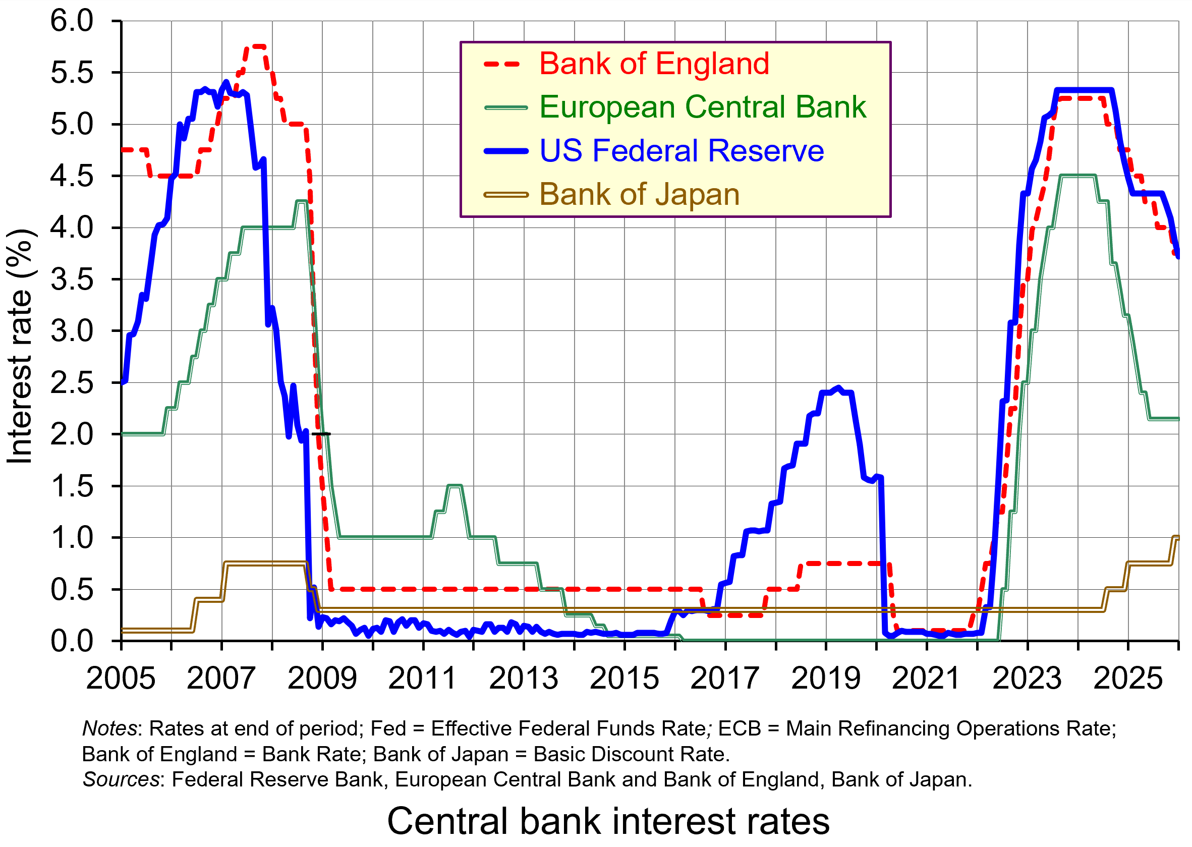
Yet President Trump is pushing the Fed to lower interest rates rapidly and despite three cuts in a row of 0.25 percentage points in the last part of 2025 (see chart below), he thinks this as too little and is annoyed by suggestions that the Fed is unlikely to lower rates again for a while. He has put great pressure on Jerome Powell, the Fed Chair, to go further and faster and has threatened to replace him before his term expires in May this year. He has also made clear that he is likely to appoint someone more willing to cutting rates.
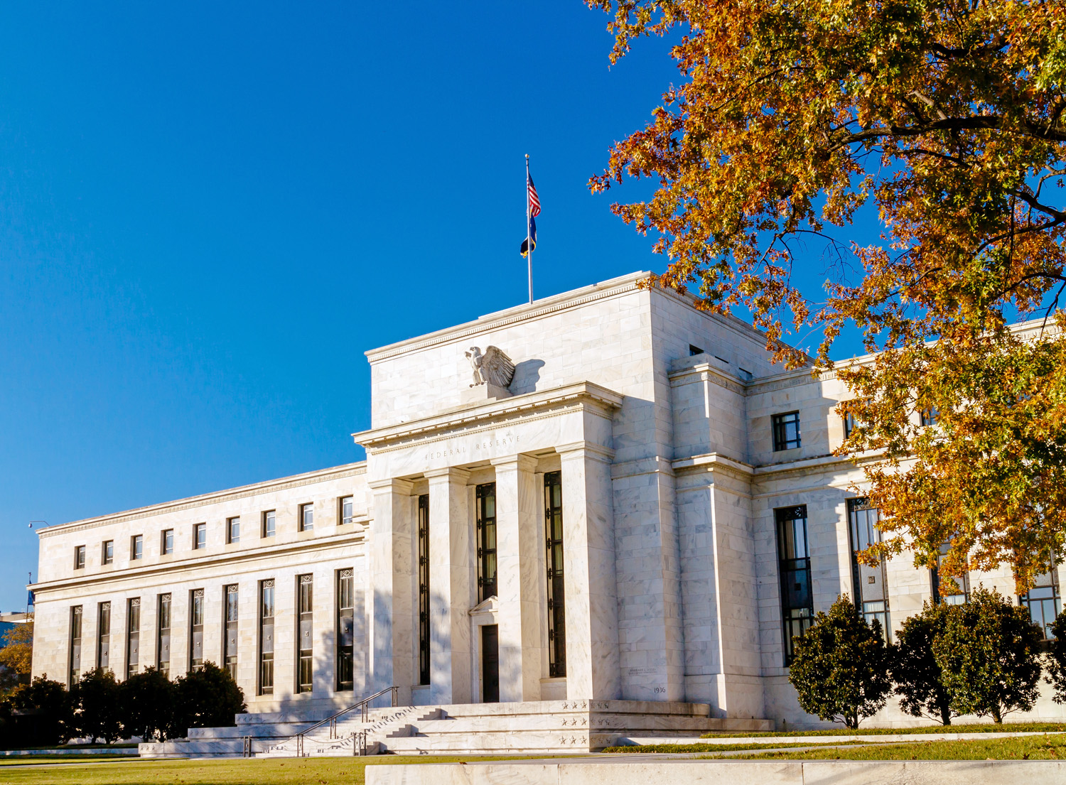
The Federal Reserve headquarters in Washington is currently being renovated. The nine-year project is costing $2.5 billion and is due to be completed next year. President Trump has declared that the project’s costs are excessive and unnecessary.
On 11 January, Federal prosecutors confirmed that they were opening a criminal investigation into Powell, accusing him of lying to Congress in his June 2025 testimony regarding the scope and costs of the renovations.
Powell responded by posting a video in which he claimed that the real reason that he was being threatened with criminal charges was not because of the renovations but because the Fed had ignored President Trump’s pressure and had set interest rates:
based on our best assessment of what will serve the public, rather than following the preferences of the President. This is about whether the Fed will be able to continue to set interest rates based on evidence and economic conditions – or whether, instead, monetary policy will be directed by political pressure or intimidation.
The Fed’s mandate
 The Federal Reserve Board decides on monetary policy and then the Federal Open Market Committee (FOMC) decides how to carry it out. It decides on interest rates and asset sales or purchases. The FOMC meets eight times a year.
The Fed is independent of both the President and Congress, and its Chair is generally regarded as having great power in determining the country’s economic policy.
Since 1977, the Fed’s statutory mandate has been to promote the goals of stable prices and maximum employment. Because of the reference to both prices and employment, the mandate is commonly referred to as a ‘dual mandate’. Its inflation target is 2 per cent over the long run with ‘well anchored’ inflationary expectations.
The dual mandate is unlike that of the Bank of England, the European Central Bank, the Bank of Japan and most other central banks, which all have a single key mandate of achieving a target of a 2 per cent annual rate of consumer price inflation over a particular time period.
With a dual mandate, the two objectives may well conflict from time to time. Moreover, changes in monetary policy affect these objectives with a lag and potentially over different time horizons. Hence, an assessment may have to be made of which is the most pressing problem. This does give some leeway in setting interest rates somewhat lower than if there were a single inflation-rate target. Nevertheless, the assessment is in terms of how best to achieve the mandate and not to meet current political goals.
Statement by former Fed Chairs and Governors
On 12 January, three former Chairs of the Federal Reserve (Janet Yellen, Ben Bernanke and Alan Greenspan), four former Treasury Secretaries (Timothy Geithner, Jacob Lew, Henry Paulson and Robert Rubin) and seven other top former economic officials issued the following statement (see Substack link in the Articles section below):
The Federal Reserve’s independence and the public’s perception of that independence are critical for economic performance, including achieving the goals Congress has set for the Federal Reserve of stable prices, maximum employment, and moderate long-term interest rates. The reported criminal inquiry into Federal Reserve Chair Jay Powell is an unprecedented attempt to use prosecutorial attacks to undermine that independence. This is how monetary policy is made in emerging markets with weak institutions, with highly negative consequences for inflation and the functioning of their economies more broadly. It has no place in the United States whose greatest strength is the rule of law, which is at the foundation of our economic success.
Response of investors
 What will happen to the dollar, US bond prices, share prices and US inflation, and what will happen to investment, depends on how people respond to the threat to the Fed’s independence. Initially, there was little response from markets, with investors probably concluding that President Trump is unlikely to be able to sway FOMC members. What is more, several Republican lawmakers have begun criticising the Trump administration’s criminal investigation, making it harder for the President to influence Fed decisions.
Even if Powell is replaced, either in the short term or in May, by a chair keen to pursue the Trump agenda, that chair will still be just one of twelve voting members of the FOMC.
Seven are appointed by the President, but serve for staggered 14-year terms. Four have been appointed by President Trump, but the other three were appointed by President Biden, although one – Lisa Cook – is being indicted by the Supreme Court for mortgage fraud, with the hearing scheduled for January 21. She claims that this is a trumped-up charge to provide grounds for removing her from the Fed. If she is removed, President Trump could appoint a replacement minded to cut rates.
The other five members include the President of the New York Fed and four of the eleven other regional Fed Presidents serving in rotation. These four are generally hawkish and would oppose early rate cuts.
Thus it is unlikely that President Trump will succeed in pushing the Fed to lower interest rates earlier than they would have done. For that reason, markets have remained relatively sanguine.
 Nevertheless, Donald Trump’s actions could well cause investors to become more worried. Will he try to find other ways to undermine the Fed? Will his actions over Venezuela, Cuba, Greenland and Iran, let alone his policies towards Ukraine and Russia and towards Israel and Gaza, heighten global uncertainty? Will his actions towards Venezuela and his desire to take over Greenland embolden China to attempt to annex Taiwan, and Russia to continue to resist plans to end the war in Ukraine or to make stronger demands?
Such developments could cause investor confidence to wane and for stock markets to fall. Time will tell. I think we need a crystal ball!
Videos
Articles
- Federal prosecutors open criminal investigation into the Fed and Jerome Powell
CNN, Bryan Mena (11/1/26)
- The Fed just gave a rare look at its $2.5 billion renovation — right before Trump’s tour
CNN, Bryan Mena (24/7/25)
- ‘A bone-headed move’: Trump’s shocking battle with Powell could badly backfire
CNN, Matt Egan (12/1/26)
- Why Powell is fighting back against Trump: The US economy is at stake
CNN, Bryan Mena (13/1/26)
- Fed chair Powell hits out at ‘unprecedented’ probe by US justice department
BBC News, Ana Faguy and Osmond Chia (12/1/26)
- Justice department opens investigation into Jerome Powell as Trump ramps up campaign against Federal Reserve
The Guardian, Callum Jones (12/1/26)
- Some Republicans speak out against DoJ investigation into Fed chair
The Guardian, Joseph Gedeon (12/1/26)
- Trump’s attempts to influence Fed risk 1970s-style inflation and global backlash
The Guardian, Richard Partington (12/1/26)
- Statement on the Federal Reserve
Substack, 14 signatories (12/1/26)
- Yellen says Powell probe ‘extremely chilling’ for Fed independence, market should be concerned
CNBC, Jeff Cox (12/1/26)
- Global central bankers unite in defense of Fed Chair Jerome Powell
CNBC, Holly Ellyatt (13/1/26)
- Trump attacks Powell again amid Fed independence fears: ‘That jerk will be gone soon’
CNBC, Kevin Breuninger (13/1/26)
- Former Fed chairs condemn criminal investigation into Jerome Powell
BBC News, Danielle Kaye (12/1/26)
- Fed: Towards a very divided Fed in the coming months and quarters
CPR AM, Bastien Drut (28/11/25)
- Treasury Yields Diverge as Powell Probe Rekindles Fed Independence Risk
Investing.com, Khasay Hashimov (12/1/26)
- Instant View: Investors react as Trump-Fed feud escalates
Reuters (12/1/26)
- Fighting the Fed, Trump tries credit easing by decree
Reuters, Mike Dolan (13/1/26)
- Trump’s attacks on the Federal Reserve risk fuelling US inflation and ending dollar dominance
The Conversation, Emre Tarim (13/1/26)
Questions
- What are the arguments for central bank independence?
- What are the arguments for control of monetary policy by the central government?
- Assess the above arguments.
- Find out what has happened to interest rates, the US stock market and the dollar since this blog was written.
- How do the fiscal decisions by government affect monetary policy?
- Compare the benefits of the dual mandate system of the Fed with those of the single mandate of the Bank of England and ECB.
 With businesses increasing their use of AI, this is likely to have significant effects on employment. But how will this affect the distribution of income, both within countries and between countries?
In some ways, AI is likely to increase inequality within countries as it displaces low-skilled workers and enhances the productivity of higher-skilled workers. In other ways, it could reduce inequality by allowing lower-skilled workers to increase their productivity, while displacing some higher-skilled workers and managers through the increased adoption of automated processes.
The effect of AI on the distribution of income between countries will depend crucially on its accessibility. If it is widely available to low-income countries, it could significantly enhance the productivity of small businesses and workers in such countries and help to reduce the income gap with the richer world. If the gains in such countries, however, are largely experienced by multinational companies, whether in mines and plantations, or in labour-intensive industries, such as garment production, few of the gains may accrue to workers and global inequality may increase.
Redistribution within a country
 The deployment of AI may result in labour displacement. AI is likely to replace both manual and white-collar jobs that involve straightforward and repetitive tasks. These include: routine clerical work, such as data entry, filing and scheduling; paralegal work, contract drafting and legal research; consulting, business research and market analysis; accounting and bookkeeping; financial trading; proofreading, copy mark-up and translation; graphic design; machine operation; warehouse work, where AI-enabled warehouse robots do many receiving, sorting, stacking, retrieval, carrying and loading tasks (e.g. Amazon’s Sequoia robotic system); basic coding or document sifting; market research and advertising design; call-centre work, such as enquiry handling, sales, telemarketing and customer service; hospitality reception; sales cashiers in supermarkets and stores; analysis of health data and diagnosis. Such jobs can all be performed by AI assistants, AI assisted robots or chat bots.
Women are likely to be disproportionately affected because they perform a higher share of the administrative and service roles most exposed to AI.
Workers displaced by AI may find that they can find employment only in lower-paid jobs. Examples include direct customer-facing roles, such as bar staff, shop assistants, hairdressers and nail and beauty consultants.
Such job displacement by AI is likely to redistribute income from relatively low-skilled labour to capital: a redistribution from wages to profits. This will tend to lead to greater inequality.
AI is also likely to lead to a redistribution of income towards certain types of high-skilled labour that are difficult to replace with AI but which could be enhanced by it. Take the case of skilled traders, such as plumbers, electricians and carpenters. They might be able to use AI in their work to enhance their productivity, through diagnosis, planning, problem-solving, measurement, etc. but the AI would not displace them. Instead, it could increase their incomes by allowing them to do their work more efficiently or effectively and thus increase their output per hour and enhance their hourly reward. Another example is architecture, where AI can automate repetitive tasks and open up new design possibilities, allowing architects to focus on creativity, flexibility, aesthetics, empathy with clients and ethical decision-making.
An important distinction is between disembodied and embodied AI investment. Disembodied AI investment could include AI ‘assistants’, such as ChatGPT and other software that can be used in existing jobs to enhance productivity. Such investment can usually be rolled out relatively quickly. Although the extra productivity may allow some reduction in the number of workers, disembodied AI investment is likely to be less disruptive than embodied AI investment. The latter includes robotics and automation, where workers are replaced by machines. This would require more investment and may be slower to be adopted.
Then there are jobs that will be created by AI. These include prompt engineers, who develop questions and prompt techniques to optimise AI output; health tech experts, who help organisations implement new medical AI products; AI educators, who train people in the uses of AI in the workplace; ethics advisors, who help companies ensure that their uses of AI are aligned with their values, responsibilities and goals; and cybersecurity experts who put systems in place to prevent AI stealing sensitive information. Such jobs may be relatively highly paid.
 In other cases, the gains from AI in employment are likely to accrue mainly to the consumer, with probably little change in the incomes of the workers themselves. This is particularly the case in parts of the public sector where wages/salaries are only very loosely related to productivity and where a large part of the work involves providing a personal service. For example, health professionals’ productivity could be enhanced by AI, which could allow faster and more accurate diagnosis, more efficient monitoring and greater accuracy in surgery. The main gainers would be the patients, with probably little change in the incomes of the health professionals themselves. Teachers’ productivity could be improved by allowing more rapid and efficient marking, preparation of materials and record keeping, allowing more time to be spent with students. Again, the main gainers would be the students, with little change in teachers’ incomes. Other jobs in this category include social workers, therapists, solicitors and barristers, HR specialists, senior managers and musicians.
Thus there is likely to be a distribution away from lower-skilled workers to both capital and higher-skilled workers who can use AI, to people who work in new jobs created by AI and to the consumers of certain services.
AI will accelerate productivity growth and, with it, GDP growth, but will probably displace workers faster than new roles emerge. This is likely to increase inequality and be a major challenge for society. Can the labour market adapt? Could the effects be modified if people moved to a four- or three-day week? Will governments introduce statutory limits to weekly working hours? Will training and education adapt to the new demands of employers?
Redistribution between countries
 AI threatens to widen the global rich–poor divide. It will give wealthier nations a productivity and innovation edge, which could displace low-skilled jobs in low-income nations. Labour-intensive production could be replaced by automated production, with the capital owned by the multinational companies of just a few countries, such as the USA and China, which between them account for 40% of global corporate AI R&D spending. For some companies, it would make sense to relocate production to rich countries, or certain wealthier developing countries, with better digital infrastructure, advanced data systems and more reliable power supply.
For other companies, however, production might still be based in low-income countries to take advantage of low-cost local materials. But there would still be a redistribution from wages in such countries to the profits of multinationals.
But it is not just in manufacturing where low-income countries are vulnerable to the integration of AI. Several countries, such as India, the Philippines, Mexico and Egypt have seen considerable investment in call centres and IT services for business process outsourcing and customer services. AI now poses a threat to employment in this industry as it has the potential to replace large numbers of workers.
AI-related job losses could exacerbate unemployment and deepen poverty in poorer countries, which, with limited resources, limited training and underdeveloped social protection systems, are less equipped to absorb economic and social shocks. This will further widen the global divide. In the case of embodied AI investment, it may only be possible in low-income countries through multinational investment and could displace many traditional jobs, with much of the benefit going in additional multinational profit.
But it is not all bad news for low-income countries. AI-driven innovations in healthcare, education, and agriculture, if adopted in poor countries, can make a significant contribution to raising living standards and can slow, or even reverse, the widening gap between rich and poor nations. Some of the greatest potential is in small-scale agriculture. Smallholders can boost crop yields though precision farming powered by AI; AI tools can help farmers buy seeds, fertilisers and animals and sell their produce at optimum times and prices; AI-enabled education tools can help farmers learn new techniques.
Articles
- New Skills and AI Are Reshaping the Future of Work
IMF Blog, Kristalina Georgieva (14/1/26)
- Generative AI: degenerative for jobs?
Bank Underground, Bank of England blog, Edward Egan (22/1/26)
- Artificial intelligence (AI) and employment
UK Parliament Research Briefing Lydia Harriss and Sam Money-Kyrle (23/12/25)
- Is Your Job AI-Proof? What to Know About AI Taking Over Jobs
Built In, Matthew Urwin (27/8/25)
- AI likely to displace jobs, says Bank of England governor
BBC News, Michael Race (19/12/25)
- These Jobs Will Fall First as AI Takes Over the Workplace
Forbes, Jack Kelly (30/4/25)
- Disrupted or displaced? How AI is shaking up jobs
exec-appointments.com, Anjli Raval (9/7/25)
- Navigate the economic risks and challenges of generative AI
EY-Parthenon, Lydia Boussour (25/6/24)
- AI Isn’t Increasing Inequality; It’s Revealing the Gaps We Haven’t Wanted to See
HR News, Mark Abbott (18/12/25)
- AI promises efficiency, but it’s also amplifying labour inequality
The Conversation, Mehnaz Rafi (3/12/25)
- 10 Jobs AI Will Replace in 2025
Live Career, Marta Bongilaj (29/12/25)
- From steam to Silicon: Why inequality persists
Aik News HD (Pakistan), Ahmed Fawad Farooq (27/12/25)
- Rethinking AI’s role in income inequality
PwC: The Leadership Agenda (4/9/25)
- How Europe Can Capture the AI Growth Dividend
IMF Blog, Florian Misch, Ben Park, Carlo Pizzinelli and Galen Sher (20/11/25)
- The Next Great Divergence
UNDP: Asia and the Pacific (2/12/25)
- AI risks sparking a new era of divergence as development gaps between countries widen, UNDP report finds
UNDP Press Release (2/12/25)
- AI threatens to widen inequality among states: UN
Aljazeera (2/12/25)
- AI risks deepening inequality, says head of world’s largest SWF
Financial Times, James Fontanella-Khan and Sun Yu (23/11/25)
- Three Reasons Why AI May Widen Global Inequality
Center for Global Development, Philip Schellekens and David Skilling (17/10/24)
- AI Will Transform the Global Economy. Let’s Make Sure It Benefits Humanity
IMF Blog, Kristalina Georgieva (14/1/24)
- AI’s $4.8 trillion future: UN Trade and Development alerts on divides, urges action
UNCTAD Press Release (7/4/25)
- AI could affect 40% of jobs and widen inequality between nations, UN warns
CNBC, Dylan Butts (4/4/25)
Questions
- What types of job are most vulnerable to AI?
- How will AI change the comparative advantage of low-income countries and what effect will it be likely to have on the pattern of global trade?
- Assess alternative policies that governments in high-income countries can adopt to offset the growth in inequality caused by the increasing use of AI.
- What policies can governments in low-income countries or aid agencies adopt to offset the growth in inequality within low-income countries and between high- and low-income countries?
- How might the growth of AI affect your own approach to career development?
- Is AI likely to increase or decrease economic power? Explain.
 The approach towards mergers remains the most controversial area of competition policy. Some argue that policy makers in both the UK and EU have been too easily persuaded by the arguments put forward by firms and so have allowed too many mergers to proceed. Others claim that the opposite is true and that merger policy has prohibited mergers that should have been allowed to proceed. This, then, has a negative impact on investment, innovation, productivity and growth.
In recent years there has been more specific criticism of merger policy in the UK. The government has indicated that it wants the Competition and Markets Authority (CMA) to be less interventionist and take a more pro-growth approach.
 In February 2025, in response to this criticism, the CMA launched its new ‘4 Ps’ approach to merger policy: Pace, Predictability, Proportionality and Process. Various changes to the investigation process have been proposed in the past 12 months using this framework.
Pace. The time taken by the CMA to initially assess a merger before deciding whether a Phase 1 investigation is necessary (i.e. the pre-notification procedure) was reduced from 65 to 40 working days. Also, the target to complete straightforward Phase 1 investigations was reduced from 35 to 25 days.
Predictability. The proposed merger guidelines, published in October 2025, provide more detail on (a) what criteria will be used to measure market shares when applying the ‘share of supply test’ (this is where the combined UK market share of two merging businesses is at least 25%, provided one business has a UK turnover of at least £10 million), and (b) the factors that are likely to lead to the competition authorities concluding that one business has gained ‘material influence over another’. Businesses had complained that there was too much uncertainty about the way the share of supply test and material influence were applied. The CMA is also considering greater alignment with other international regulators over decision making rather than its previous policy of acting independently. All these measures should increase the predictability of the investigation process.
 Proportionality. Proportionality refers to the objective of addressing any competition issues in merger cases in a way that places the minimum burden on the businesses involved. To improve proportionality, the CMA has indicated that in future cases it will be more willing to use behavioural remedies – requiring firms to take or desist from certain actions. New draft guidelines identify more situations where the use of behavioural remedies may be appropriate. However, they also show that the CMA still views structural remedies (e.g. preventing the merger or requiring firms to demerge or to sell certain assets) as more effective in many situations. Another important measure to improve proportionality is the introduction of a new ‘wait and see’ approach to global mergers. The CMA will now wait to see if the actions taken by other competition authorities in global cases address any concerns in the UK market before deciding whether to launch a review.
Process. To improve the process, the CMA has announced plans to engage with businesses at a much earlier point in the process. For example, it has pledged to share its provisional thinking in the early stages of an investigation by implementing new ‘teach-in’ sessions and having more regular update meetings. Much earlier meetings that focus on possible remedies will also take place. This may make it possible for the CMA to assess the suitability of more complex remedies during a Phase 1 investigation rather than having to wait for a longer and more costly Phase 2 review. Phase 2 reviews will also no longer be managed by panels of independent experts. This role will now be carried out by the internal CMA board.
Some critics argue that the CMA has not fully considered the potential benefits of mergers in many cases. For example, a merger could (a) have procompetitive effects, known as rivalry enhancing efficiencies (REEs) and/or (b) benefits for consumers outside of the relevant market, known as relevant customer benefits (RCBs). In response to this criticism, the CMA is currently reassessing its approach to including evidence on REEs and RCBs.
The CMA is still currently consulting with interested parties about many of these proposed changes. It will be interesting to see what final decisions are made in the next couple of years.
Articles
- CMA consults on proposed changes to its merger remedies approach
CMA Press Release (15/10/25)
- New CMA proposals to drive growth, investment and business confidence
CMA Blog, Sarah Cardell (CMA Chief Executive) (13/2/25)
- Promoting competition and protecting consumers to drive growth and improve household prosperity
CMA Speech, Sarah Cardell (20/11/25)
- Steering the course: how the CMA is responding to the Government’s pro-growth agenda
Macfarlanes (21/2/25)
- 4Ps and 3 themes – An overview of the CMA’s merger remedies review
Hogan Lovells, Angus Coulter, Alice Wallace-Wright, Karman Gordon, and Denise Hotham-Kellner (1/4/25)
- CMA publishes updated guidance on UK merger procedure
Ashurst, Christopher Eberhardt, Emile Abdul-Wahab and Finlay Sadler-Wilson (11/11/25)
- Government ousts UK competition watchdog chair
BBC News, Simon Jack and Charlotte Edwards (21/1/25)
- UK competition watchdog drops Microsoft-OpenAI probe
BBC News, Imran Rahman-Jones (5/3/25)
- Does the government really know what it wants from the CMA?
The Guardian, Nils Pratley (13/2/25)
- This article is more than 9 months old ‘We must avoid a chilling effect’: the CMA chief on the UK’s pro-growth shift
The Guardian, John Collingridge (18/2/25)
- The CMA should be nudged on antitrust, not bullied
The Financial Times, John Gapper (6/2/25)
CMA documentation
Questions
- Of all the mergers considered by the CMA in 2024/25, find out what percentage were formally investigated. How many were blocked from taking place? Do you believe that this indicates that merger policy is too weak or too strong?
- What three criteria must be met for a business arrangement to be classed as a ‘relevant merger situation’ by the CMA?
- Identify some different methods that one business could use to gain material influence over the way another company operates.
- Outline the ‘turnover test’, the ‘share of supply test’ and the ‘hybrid test’.
- Discuss the potential advantages of using behavioural remedies as opposed to structural remedies in merger cases. Why has the CMA still preferred the use of structural remedies in most situations?
 This Christmas, more people are considering giving second-hand (or ‘pre-loved’) goods as presents. This allows them to afford better-quality presents and to save money at a time when a large proportion of the population are finding that their finances are stretched. This continues a trend towards buying second-hand products – a trend driven by the rise of various online retailers, such as Vinted and Preloved, and a growing online presence of charity shops, as well as extensive use of established platforms, such as Facebook Marketplace, eBay, Depop, Gumtree and Nextdoor.
Clearly, people gain from buying and selling second-hand items – part of the ‘circular economy’. But what are the implications for gross domestic product (GDP)? After all, GDP is one of the main indicators of the size of an economy, and growth in GDP is probably the most widely-used measure of economic progress. Are second-hand transactions captured in GDP?
If you directly sell your own second-hand items, this does not count towards GDP. There is no new product being made. The items are only counted when they are first produced. Any service you provide to the purchaser (and to yourself) is in a similar category to housework, childcare, DIY and other services that people provide to themselves, household members and friends. But like such services, there is a strong argument that they should be.
 Likewise, the environmental benefits (positive externalities) of recycling products, rather than throwing them away or hoarding them, are not counted. In fact, if reusing products causes fewer new products to be made, this would be counted as subtracting from GDP.
If, however, you set up a business by buying and selling second-hand items, the service you provide would contribute towards GDP. What would be counted would the value added to the product – captured through the difference in the purchase and selling prices. In fact, HMRC has warned people that buying and selling second-hand items is taxable, as it counts as self-employment for tax purposes. But it is only this value added that counts. If you buy an item on Vinted, only the value added by Vinted counts towards GDP.
As no production takes place, the purchase of second-hand items adds either nothing to GDP or just the service of a retailer. It is effectively just a transfer of goods and money. If buying second-hand items means that you buy fewer new ones, then that would cause GDP to fall if the response of firms is to produce fewer newer items. However, the person selling the second-hand items will gain revenue, which could be used to buy new items. If that increased production, that would boost GDP. The net effect on GDP of this transfer of goods and money in the second-hand market will be pretty small.
Yet, clearly, the second-hand market provides a welfare gain to both sellers and purchasers – a gain that is likely to grow as the use of second-hand markets increases. At Christmas time, it provides a timely warning of the limitations of using GDP to measure wellbeing.
Articles
- Giving toys another life with another child
Westmorland & Furness Council, News (18/11/25)
- ‘I make £1,000 a week with charity shop side hustle – I couldn’t afford Christmas without it’
Manchester Evening News, Lee Grimsditch and Hannah Cottrell (3/12/25)
- HMRC issues warning to anyone with money-making ‘side hustle’ ahead of Christmas
Manchester Evening News , Ryan Price (12/11/25)
- 12 tips for a low cost Christmas
Rest Less, Melanie Wright (14/11/25)
- I’ve saved over £100 on my girl’s Christmas gifts & got everything on her list including Disney dolls & Hey Dugee toys
The Sun, Becky Pemberton (25/11/25)
- Circular trade is growing, but will second-hand shopping be visible during the Christmas season?
Finnish Commerce Federation, Press Release (27/11/25)
- Shop secondhand, shred your veg and try ‘furoshiki’ wrapping: 14 easy ways to cut Christmas waste
The Guardian, Hannah Rochell (8/12/25)
- 13 Ways to Have a Sustainable Christmas This Year
Circular&Co., Adam Millett (1/12/23)
- The Role of Circular Economy in Driving Economic Growth: Evidence from EU Countries
Sage Open, Vladimir Radivojević, Tamara Rađenović and Jelena Dimovski (14/11/24)
- How to Have a Circular Economy Christmas: Deck the Halls, Sustainably
50 Shades Greener, Kiri Spanowicz (10/12/24)
- Twelve Economic Impacts of Christmas
City-REDI Blog, Birmingham University, Charlotte Hoole (22/12/16)
- Christmas 2025: Christmas Economics Explained
Plus500 (23/11/25)
Questions
- What other items or activities affecting human wellbeing are not counted in GDP?
- Name some goods and services that are produced, and hence are included in GDP, but which can be classed as ‘bads’.
- For what reasons might a country have a high GDP per capita but a poor average level of wellbeing?
- How might GDP figures be adjusted for international comparison purposes?
- Would it be possible to adjust GDP figures to take account of externalities in production (negative and positive)? If so, how?
- Production involves human costs. To what extent does GDP take this into account?
- What is meant by the circular economy? How might you have a ‘circular’ Christmas?
 The share prices of various AI-related companies have soared in this past year. Recently, however, they have fallen – in some cases dramatically. Is this a classic case of a bubble that is bursting, or at least deflating?
Take the case of NVIDIA, the world’s most valuable company, with a market capitalisation of around $4.2 trillion (at current share prices). It designs and produces graphics cards and is a major player in AI. From a low of $86.62 April this year, its share price rose to a peak of $212.19 on 29 October. But then began falling as talk grew of an AI bubble. Despite news on 19 November that its 2025 Q3 earnings were up 62% to $57.0bn, beating estimates by 4%, its share price, after a temporary rise, began falling again. By 21 November, it was trading at around $180.
Other AI-related stocks have seen much bigger rises and falls. One of the biggest requirements for an AI revolution is data processing, which uses huge amounts of electricity. Massive data centres are being set up around the world. Several AI-related companies have been building such data centres. Some were initially focused largely on ‘mining’ bitcoin and other cryptocurrencies (see the blog, Trump and the market for crypto). But many are now changing focus to providing processing power for AI.
 Take the case of the Canadian company, Bitfarms Ltd. As it says on its site: ‘With access to multiple energy sources and strategic locations, our U.S. data centers support both mining and high-performance computing growth opportunities’. Bitfarms’ share price was around CAD1.78 in early August this year. By 15 October, it had reached CAD9.27 – a 421% increase. It then began falling and by 24 November was CAD3.42 – a decline of over 63%.
Data centres do have huge profit potential as the demand for AI increases. Many analysts are arguing that the current share price of data centres undervalues their potential. But current profits of such companies are still relatively low, or they are currently loss making. This then raises the question of how much the demand for shares, and hence their price, depends on current profits or future potential. And a lot here depends on sentiment.
If people are optimistic, they will buy and this will lead to speculation that drives up the share price. If sentiment then turns and people believe that the share price is overvalued, with future profits too uncertain or less than previously thought, or if they simply believe that the share price has overshot the value that reflects a realistic profit potential, they will sell and this will lead to speculation that drives down the share price
 The dot.com bubble of the late 1990s/early 2000s is a case in point. There was a stock market bubble from roughly 1995 to 2001, where speculative investment in internet-based companies caused their stock values to surge, peaking in late 1999/early 2000. There was then a dramatic crash. But then years later, many of these companies’ share prices had risen well above their peak in 2000.
Take the case of Amazon. In June 1997, its share price was $0.08. By mid-December 1999, it had reached $5.65. It then fell, bottoming out at $0.30 in September 2001. The dot-com bubble had burst.
But the potential foreseen in many of these new internet companies was not wrong. After 2001, Amazon’s share price began rising once more. Today, Amazon’s shares are trading at over $200 – the precise value again being driven largely by the company’s performance and potential and by sentiment.
So is the boom in AI-related stock a bubble? Given that the demand for AI is likely to continue growing rapidly, it is likely that the share price of companies providing components and infrastructure for AI is likely to continue growing in the long term. But just how far their share prices will fall in the short term is hard to call. Sentiment is a fickle thing.
Articles
Questions
- Using a supply and demand diagram, illustrate how speculation can drive up the share price of a company and then result in it falling.
- What is meant by overshooting in a market? What is the role of speculation in this process?
- Does a rapid rise in the price of an asset always indicate a bubble? Explain.
- What are the arguments for suggesting that markets are/are not experiencing an AI share price bubble? Does it depend of what part of the AI market is being considered?
- What is meant by the market capitalisation of a company? Is it a good basis for deciding whether or not a company’s share price is a true reflection of the company’s worth? What other information would you require?
- Find out what has been happening to the price of Bitcoin. What factors determine the price of Bitcoin? Do these factors make the price inherently unstable?
 Donald Trump is keen to lower US interest rates substantially and rapidly in order to provide a boost to the US economy. He is also keen to reduce the cost of living for US citizens and sees lower interest rates as a means of reducing the burden of debt servicing for both consumers and firms alike.
 The Federal Reserve Board decides on monetary policy and then the Federal Open Market Committee (FOMC) decides how to carry it out. It decides on interest rates and asset sales or purchases. The FOMC meets eight times a year.
  What will happen to the dollar, US bond prices, share prices and US inflation, and what will happen to investment, depends on how people respond to the threat to the Fed’s independence. Initially, there was little response from markets, with investors probably concluding that President Trump is unlikely to be able to sway FOMC members. What is more, several Republican lawmakers have begun criticising the Trump administration’s criminal investigation, making it harder for the President to influence Fed decisions.
 Nevertheless, Donald Trump’s actions could well cause investors to become more worried. Will he try to find other ways to undermine the Fed? Will his actions over Venezuela, Cuba, Greenland and Iran, let alone his policies towards Ukraine and Russia and towards Israel and Gaza, heighten global uncertainty? Will his actions towards Venezuela and his desire to take over Greenland embolden China to attempt to annex Taiwan, and Russia to continue to resist plans to end the war in Ukraine or to make stronger demands?
 Statement from Federal Reserve Chair Jerome H. Powell
 Trump’s intimidation of Fed’s leadership threatens economic stability, Yellen says
 Janet Yellen says Powell probe ‘extremely chilling’ for Fed independence, market should be concerned
 Treasury Secretary Scott Bessent is reportedly unhappy with criminal investigation of Fed Chair Jerome Powell
 With businesses increasing their use of AI, this is likely to have significant effects on employment. But how will this affect the distribution of income, both within countries and between countries?
 The deployment of AI may result in labour displacement. AI is likely to replace both manual and white-collar jobs that involve straightforward and repetitive tasks. These include: routine clerical work, such as data entry, filing and scheduling; paralegal work, contract drafting and legal research; consulting, business research and market analysis; accounting and bookkeeping; financial trading; proofreading, copy mark-up and translation; graphic design; machine operation; warehouse work, where AI-enabled warehouse robots do many receiving, sorting, stacking, retrieval, carrying and loading tasks (e.g. Amazon’s Sequoia robotic system); basic coding or document sifting; market research and advertising design; call-centre work, such as enquiry handling, sales, telemarketing and customer service; hospitality reception; sales cashiers in supermarkets and stores; analysis of health data and diagnosis. Such jobs can all be performed by AI assistants, AI assisted robots or chat bots.
 In other cases, the gains from AI in employment are likely to accrue mainly to the consumer, with probably little change in the incomes of the workers themselves. This is particularly the case in parts of the public sector where wages/salaries are only very loosely related to productivity and where a large part of the work involves providing a personal service. For example, health professionals’ productivity could be enhanced by AI, which could allow faster and more accurate diagnosis, more efficient monitoring and greater accuracy in surgery. The main gainers would be the patients, with probably little change in the incomes of the health professionals themselves. Teachers’ productivity could be improved by allowing more rapid and efficient marking, preparation of materials and record keeping, allowing more time to be spent with students. Again, the main gainers would be the students, with little change in teachers’ incomes. Other jobs in this category include social workers, therapists, solicitors and barristers, HR specialists, senior managers and musicians.
 AI threatens to widen the global rich–poor divide. It will give wealthier nations a productivity and innovation edge, which could displace low-skilled jobs in low-income nations. Labour-intensive production could be replaced by automated production, with the capital owned by the multinational companies of just a few countries, such as the USA and China, which between them account for 40% of global corporate AI R&D spending. For some companies, it would make sense to relocate production to rich countries, or certain wealthier developing countries, with better digital infrastructure, advanced data systems and more reliable power supply.
 The approach towards mergers remains the most controversial area of competition policy. Some argue that policy makers in both the UK and EU have been too easily persuaded by the arguments put forward by firms and so have allowed too many mergers to proceed. Others claim that the opposite is true and that merger policy has prohibited mergers that should have been allowed to proceed. This, then, has a negative impact on investment, innovation, productivity and growth.
 In February 2025, in response to this criticism, the CMA launched its new ‘4 Ps’ approach to merger policy: Pace, Predictability, Proportionality and Process. Various changes to the investigation process have been proposed in the past 12 months using this framework.
  Proportionality. Proportionality refers to the objective of addressing any competition issues in merger cases in a way that places the minimum burden on the businesses involved. To improve proportionality, the CMA has indicated that in future cases it will be more willing to use behavioural remedies – requiring firms to take or desist from certain actions. New draft guidelines identify more situations where the use of behavioural remedies may be appropriate. However, they also show that the CMA still views structural remedies (e.g. preventing the merger or requiring firms to demerge or to sell certain assets) as more effective in many situations. Another important measure to improve proportionality is the introduction of a new ‘wait and see’ approach to global mergers. The CMA will now wait to see if the actions taken by other competition authorities in global cases address any concerns in the UK market before deciding whether to launch a review.
  This Christmas, more people are considering giving second-hand (or ‘pre-loved’) goods as presents. This allows them to afford better-quality presents and to save money at a time when a large proportion of the population are finding that their finances are stretched. This continues a trend towards buying second-hand products – a trend driven by the rise of various online retailers, such as Vinted and Preloved, and a growing online presence of charity shops, as well as extensive use of established platforms, such as Facebook Marketplace, eBay, Depop, Gumtree and Nextdoor.
 Likewise, the environmental benefits (positive externalities) of recycling products, rather than throwing them away or hoarding them, are not counted. In fact, if reusing products causes fewer new products to be made, this would be counted as subtracting from GDP.
 Take the case of the Canadian company,
  The dot.com bubble of the late 1990s/early 2000s is a case in point. There was a stock market bubble from roughly 1995 to 2001, where speculative investment in internet-based companies caused their stock values to surge, peaking in late 1999/early 2000. There was then a dramatic crash. But then years later, many of these companies’ share prices had risen well above their peak in 2000.