 Wobbles in the private credit market in the fourth quarter of 2025 spooked those retail investors with investments in private credit funds – a significant segment of the growing shadow banking sector. These funds use investors’ money to finance lending to businesses and individuals who struggle to, or do not want to, access credit from banks and the public market. Therefore, the risks are higher.
The failures of two auto parts suppliers in the USA last year have highlighted the risks involved. Retail investors are exiting such funds in significant numbers. Bcred, Blackstone’s $82 billion private credit fund, saw money equivalent to 8% of its net asset value (NAV) withdrawn. The firm, and employees, put $400m in to maintain confidence.
Blue Owl, another credit manager, closed investors’ usual quarterly redemption window, largely due to unprecedented demand. The fund’s managers have decided that they will wind down the fund and return money back to investors over time, whether that want it or not.
Several other listed funds run by big names, such as Blackrock and KKR, have slashed dividends and written down asset values. This week, both Morgan Stanley and Cliffwater limited withdrawals from their credit funds.
So, what has happened? In recent years, there has been a big growth in private credit funds in the USA aimed at individual retail investors. With interest margins low and fees from public investment products diminishing due to the shift to passive investing, financial institutions spied an opportunity for chunky fees by offering private credit investment to retail investors.
The liquidity–return trade-off
 Such investors are attracted by the potential for higher returns that private credit funds offered compared to public funds. The need to provide higher returns was related partly to the higher credit risk associated with the lending, but also to the illiquidity of the private credit assets that the funds invested in.
While much attention in the financial media has focused on the heightened credit risk in private funds, less attention has been given to the liquidity issue. At the heart of the private credit business model is a level of illiquidity that individual retail investors would not be comfortable with. The liquidity–return trade-off is one of the fundamental concepts in finance. Investors must be prepared to trade-off liquidity for higher returns, and vice versa. They cannot have both.
This blog will discuss that trade-off in the context of private credit funds and its lessons for retail investors, particularly in Europe where institutions are gearing up to offer such investment products.
Liquidity preference
One of the fundamental concepts in finance is the maturity mismatch between the preferences of ultimate lenders (typically households) and the requirements of ultimate borrowers (typically firms, but also households and governments too). Typically, lenders want to ‘lend short’ while borrowers want to ‘borrow long’. The financial system reconciles this mismatch by providing two important economic functions – maturity transformation and liquidity provision.
 Banks offer maturity transformation by offering current and other accounts to individuals where deposits can be redeemed at short notice. These institutions use the deposits to finance long-term lending for a variety of purposes; examples include property, investment in capital or day-to-day spending. Their effective management of this process is important economically for the smooth running of the payments mechanism and for economic growth.
But, to fulfil this, banks have to hold a mixture of assets with varying degrees of liquidity – some highly liquid, such as cash and short-term government debt instruments, and some illiquid, such as long-term loans. Liquidity is such an important issue for banks that their assets are listed on their balance sheet in order of liquidity – from most liquid to least liquid.
However, there is an inverse relationship between liquidity and expected return. Banks and their customers have to sacrifice return if they want higher liquidity. Therefore, liquid assets tend to offer a low rate of return and illiquid assets a higher rate of return. Consequently, in order to retain sufficient liquidity, the overall return banks can generate is limited compared to a situation where they invest wholly in illiquid assets.
If individuals want to invest directly in long-term financial assets, such as debt and equity, there must be a secondary market where these can be bought and sold – the stock market. Without this mechanism providing liquidity, individuals are less likely to invest in these assets in the first place. Few would want to wait for a debt security to mature or hold a share in perpetuity. Secondary markets mean they don’t have to.
Liquidity and private credit
Private credit funds have existed for a long time as part of the shadow banking sector and have grown in scale. Such funds invest in non-tradable, long-term illiquid loans as a parallel to the better-known private equity sector. Traditionally they have been targeted at institutional investors, who are more comfortable with the higher credit risk and illiquidity involved.
However, while institutions are prepared to forgo liquidity for many years in expectation of higher returns, individual retail investors are not – they have a higher liquidity preference. Funds tailoring private credit funds acknowledged that individual investors required a liquidity incentive to invest. Since there is no liquid secondary market to facilitate liquidation, private funds aimed at such retail investors offered quarterly redemption opportunities. The industry standard settled on around 5% of a fund’s value.
However, offering these ‘liquidity windows’ creates a tension in the private credit business model. Private credit operates on the basis of illiquidity in return for higher returns. This includes borrowers prepared to pay a higher interest rate on debt to avoid exposure to the glare of public market scrutiny.
Further, the prices of private loans are not ‘marked-to-the-market’ like publicly traded debt, so they are not correlated with public markets. This enables fund managers to work out credit problems over time rather than be forced into fire sales to meet the liquidity needs of investors.
 Offering liquidity confounds that. To do so, private credit funds end up operating like quasi-public funds. They have to hold sufficient liquid assets to cover redemptions. Indeed, regulations for such funds in Europe are proposing a minimum of 20% of assets in liquid investments so there is a reserve to meet redemptions. But, by doing so, funds will not be able to generate the promised returns. Indeed, returns may be not much higher that that offered by public traded funds.
Further, providing quarterly redemption windows requires fair and timely valuations of the fund. Irrespective of perceptions around credit risk, if investors feel that the valuation is generous then many will want to take advantage of the liquidity window to redeem and no limit on withdrawals, be it 5%, 10% or whatever, is sufficient. However, with no secondary market mechanism to remove the excess demand, those told they cannot redeem their investment will only increase their demands for liquidity further and exit at the next available opportunity.
This irreconcilable tension in offering private credit funds to retail investors is being recognised. Not only are funds like Blue Owl being wound up, but the share prices of providers in the USA have fallen sharply as markets realise that the anticipated returns from selling private credit to retail investors are unlikely to be realised. Blackstone’s market capitalisation has halved from $250 billion at the end of 2024 to $134 billion on 11 March 2026.
But this is the moment when private credit funds are being offered to retail investors in Europe. The lesson for European retail investors from the US experience is that you can’t have high liquidity and high return. As with most allocation decisions, there is a trade-off.
Articles
Questions
- What is maturity transformation? Explain how banks conduct maturity transformation.
- What is liquidity provision? Explain how secondary financial markets provide liquidity.
- Explain why private credit funds offer a higher expected return than public ones?
- Analyse the pressures on profit margins in public markets which led financial institutions to offer private credit funds. In doing so, consider the ethics around offering such a product to retail investors.
- Explain why offering such funds to individual (retail) investors has not worked.
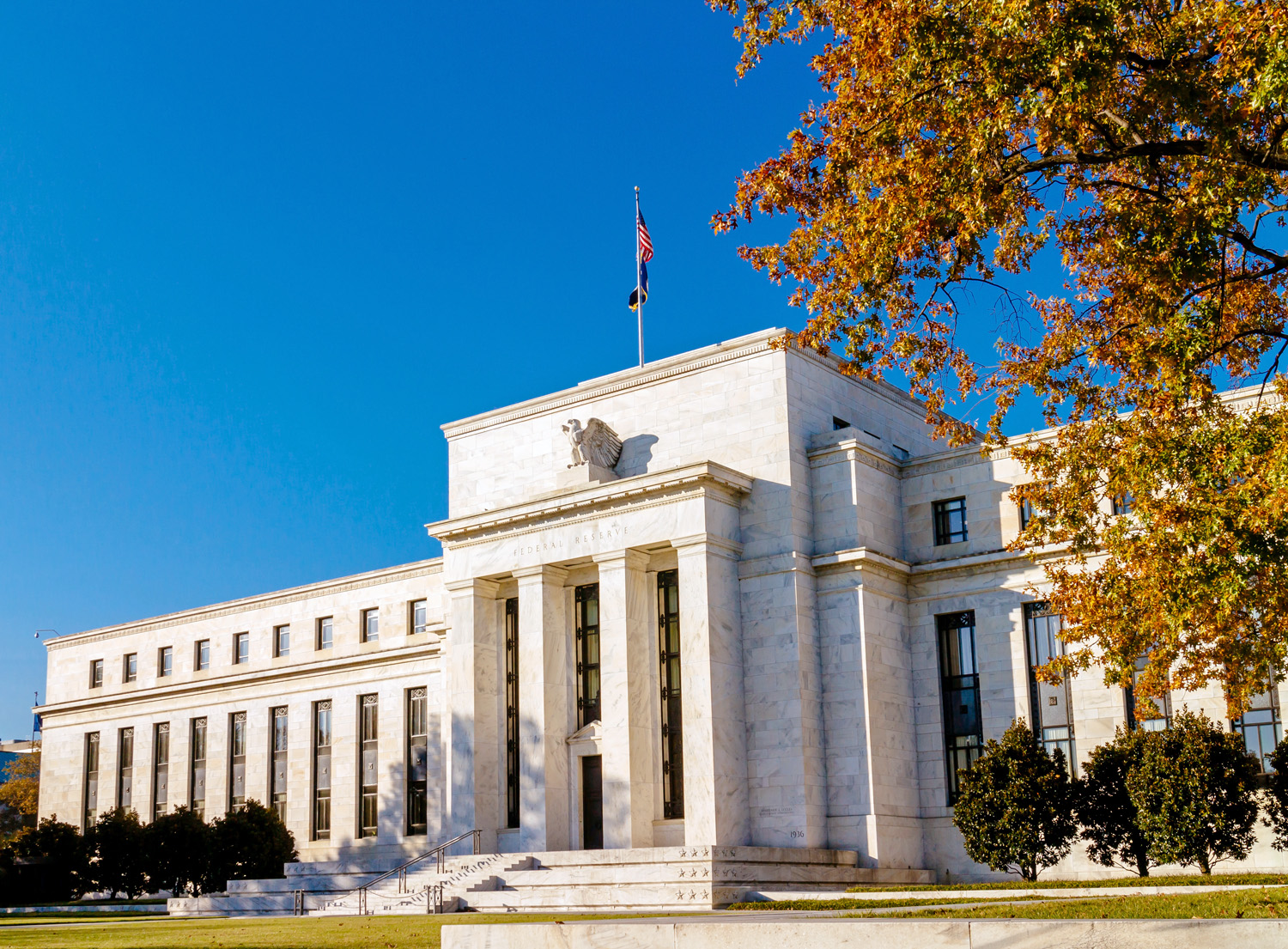 Donald Trump is keen to lower US interest rates substantially and rapidly in order to provide a boost to the US economy. He is also keen to reduce the cost of living for US citizens and sees lower interest rates as a means of reducing the burden of debt servicing for both consumers and firms alike.
But interest rates are set by the US central bank, the Federal Reserve (the ‘Fed’), which is formally independent from government. This independence is seen as important for providing stability to the US economy and removing monetary policy from short-term political pressures to cut interest rates. Succumbing to political pressures would be likely to create uncertainty and damage long-term stability and growth.
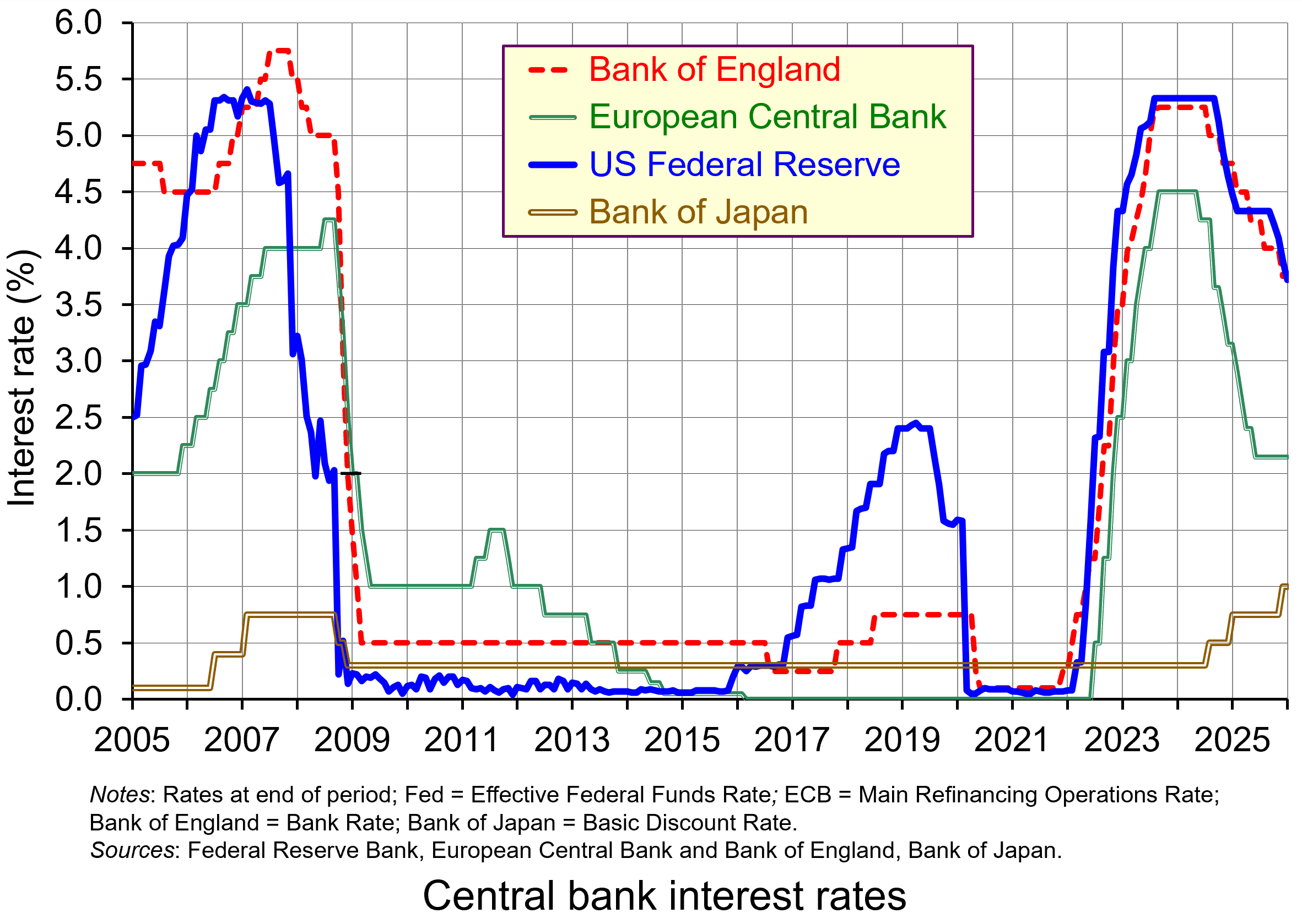
Yet President Trump is pushing the Fed to lower interest rates rapidly and despite three cuts in a row of 0.25 percentage points in the last part of 2025 (see chart below), he thinks this as too little and is annoyed by suggestions that the Fed is unlikely to lower rates again for a while. He has put great pressure on Jerome Powell, the Fed Chair, to go further and faster and has threatened to replace him before his term expires in May this year. He has also made clear that he is likely to appoint someone more willing to cutting rates.
The Federal Reserve headquarters in Washington is currently being renovated. The nine-year project is costing $2.5 billion and is due to be completed next year. President Trump has declared that the project’s costs are excessive and unnecessary.
On 11 January, Federal prosecutors confirmed that they were opening a criminal investigation into Powell, accusing him of lying to Congress in his June 2025 testimony regarding the scope and costs of the renovations.
Powell responded by posting a video in which he claimed that the real reason that he was being threatened with criminal charges was not because of the renovations but because the Fed had ignored President Trump’s pressure and had set interest rates:
based on our best assessment of what will serve the public, rather than following the preferences of the President. This is about whether the Fed will be able to continue to set interest rates based on evidence and economic conditions – or whether, instead, monetary policy will be directed by political pressure or intimidation.
The Fed’s mandate
 The Federal Reserve Board decides on monetary policy and then the Federal Open Market Committee (FOMC) decides how to carry it out. It decides on interest rates and asset sales or purchases. The FOMC meets eight times a year.
The Fed is independent of both the President and Congress, and its Chair is generally regarded as having great power in determining the country’s economic policy.
Since 1977, the Fed’s statutory mandate has been to promote the goals of stable prices and maximum employment. Because of the reference to both prices and employment, the mandate is commonly referred to as a ‘dual mandate’. Its inflation target is 2 per cent over the long run with ‘well anchored’ inflationary expectations.
The dual mandate is unlike that of the Bank of England, the European Central Bank, the Bank of Japan and most other central banks, which all have a single key mandate of achieving a target of a 2 per cent annual rate of consumer price inflation over a particular time period.
With a dual mandate, the two objectives may well conflict from time to time. Moreover, changes in monetary policy affect these objectives with a lag and potentially over different time horizons. Hence, an assessment may have to be made of which is the most pressing problem. This does give some leeway in setting interest rates somewhat lower than if there were a single inflation-rate target. Nevertheless, the assessment is in terms of how best to achieve the mandate and not to meet current political goals.
Statement by former Fed Chairs and Governors
On 12 January, three former Chairs of the Federal Reserve (Janet Yellen, Ben Bernanke and Alan Greenspan), four former Treasury Secretaries (Timothy Geithner, Jacob Lew, Henry Paulson and Robert Rubin) and seven other top former economic officials issued the following statement (see Substack link in the Articles section below):
The Federal Reserve’s independence and the public’s perception of that independence are critical for economic performance, including achieving the goals Congress has set for the Federal Reserve of stable prices, maximum employment, and moderate long-term interest rates. The reported criminal inquiry into Federal Reserve Chair Jay Powell is an unprecedented attempt to use prosecutorial attacks to undermine that independence. This is how monetary policy is made in emerging markets with weak institutions, with highly negative consequences for inflation and the functioning of their economies more broadly. It has no place in the United States whose greatest strength is the rule of law, which is at the foundation of our economic success.
Response of investors
 What will happen to the dollar, US bond prices, share prices and US inflation, and what will happen to investment, depends on how people respond to the threat to the Fed’s independence. Initially, there was little response from markets, with investors probably concluding that President Trump is unlikely to be able to sway FOMC members. What is more, several Republican lawmakers have begun criticising the Trump administration’s criminal investigation, making it harder for the President to influence Fed decisions.
Even if Powell is replaced, either in the short term or in May, by a chair keen to pursue the Trump agenda, that chair will still be just one of twelve voting members of the FOMC.
Seven are appointed by the President, but serve for staggered 14-year terms. Four have been appointed by President Trump, but the other three were appointed by President Biden, although one – Lisa Cook – is being indicted by the Supreme Court for mortgage fraud, with the hearing scheduled for January 21. She claims that this is a trumped-up charge to provide grounds for removing her from the Fed. If she is removed, President Trump could appoint a replacement minded to cut rates.
The other five members include the President of the New York Fed and four of the eleven other regional Fed Presidents serving in rotation. These four are generally hawkish and would oppose early rate cuts.
Thus it is unlikely that President Trump will succeed in pushing the Fed to lower interest rates earlier than they would have done. For that reason, markets have remained relatively sanguine.
 Nevertheless, Donald Trump’s actions could well cause investors to become more worried. Will he try to find other ways to undermine the Fed? Will his actions over Venezuela, Cuba, Greenland and Iran, let alone his policies towards Ukraine and Russia and towards Israel and Gaza, heighten global uncertainty? Will his actions towards Venezuela and his desire to take over Greenland embolden China to attempt to annex Taiwan, and Russia to continue to resist plans to end the war in Ukraine or to make stronger demands?
Such developments could cause investor confidence to wane and for stock markets to fall. Time will tell. I think we need a crystal ball!
Videos
Articles
- Federal prosecutors open criminal investigation into the Fed and Jerome Powell
CNN, Bryan Mena (11/1/26)
- The Fed just gave a rare look at its $2.5 billion renovation — right before Trump’s tour
CNN, Bryan Mena (24/7/25)
- ‘A bone-headed move’: Trump’s shocking battle with Powell could badly backfire
CNN, Matt Egan (12/1/26)
- Why Powell is fighting back against Trump: The US economy is at stake
CNN, Bryan Mena (13/1/26)
- Fed chair Powell hits out at ‘unprecedented’ probe by US justice department
BBC News, Ana Faguy and Osmond Chia (12/1/26)
- Justice department opens investigation into Jerome Powell as Trump ramps up campaign against Federal Reserve
The Guardian, Callum Jones (12/1/26)
- Some Republicans speak out against DoJ investigation into Fed chair
The Guardian, Joseph Gedeon (12/1/26)
- Trump’s attempts to influence Fed risk 1970s-style inflation and global backlash
The Guardian, Richard Partington (12/1/26)
- Statement on the Federal Reserve
Substack, 14 signatories (12/1/26)
- Yellen says Powell probe ‘extremely chilling’ for Fed independence, market should be concerned
CNBC, Jeff Cox (12/1/26)
- Global central bankers unite in defense of Fed Chair Jerome Powell
CNBC, Holly Ellyatt (13/1/26)
- Trump attacks Powell again amid Fed independence fears: ‘That jerk will be gone soon’
CNBC, Kevin Breuninger (13/1/26)
- Former Fed chairs condemn criminal investigation into Jerome Powell
BBC News, Danielle Kaye (12/1/26)
- Fed: Towards a very divided Fed in the coming months and quarters
CPR AM, Bastien Drut (28/11/25)
- Treasury Yields Diverge as Powell Probe Rekindles Fed Independence Risk
Investing.com, Khasay Hashimov (12/1/26)
- Instant View: Investors react as Trump-Fed feud escalates
Reuters (12/1/26)
- Fighting the Fed, Trump tries credit easing by decree
Reuters, Mike Dolan (13/1/26)
- Trump’s attacks on the Federal Reserve risk fuelling US inflation and ending dollar dominance
The Conversation, Emre Tarim (13/1/26)
Questions
- What are the arguments for central bank independence?
- What are the arguments for control of monetary policy by the central government?
- Assess the above arguments.
- Find out what has happened to interest rates, the US stock market and the dollar since this blog was written.
- How do the fiscal decisions by government affect monetary policy?
- Compare the benefits of the dual mandate system of the Fed with those of the single mandate of the Bank of England and ECB.
Large European banks call for further integration, but is it in consumers’ interests?
 Those of a certain age may remember the fanfare which heralded the introduction of the Single European market (SEM) on 1 January 1993. It promised the removal of internal barriers to the movement of goods, services, capital and people. One sector that was noticeably absent from the single market, however, was banking.
Moves towards banking union only started after the global financial crisis in 2008. However, as a report published on the 2 September 2025 by the Association of Financial Markets in Europe (AFME) highlights, the institutional frameworks of banking in the EU are still deeply fragmented – the promised integration through the European Banking Union (EBU) is still incomplete. This has put European banks at a competitive disadvantage in global markets compared with rivals from the USA and Asia, thereby reducing their profitability and growth prospects. The report called on the European Central Bank (ECB) and national regulatory authorities to remove hurdles to cross-border banking services in the EU. This would enhance the strategic position of European banks.
In this blog we will trace the development of the EBU and analyse the current state of integration. We discuss the AFME proposals for achieving greater integration and highlight their benefits for large banks. We also analyse the barriers which limit full integration and examine the risks that retail customers might see few benefits from the proposed changes.
What is meant by European Banking Union (EBU)?
The 1993 Single European Market (SEM) in goods and services removed internal barriers to the movement of goods, services, capital and people within the EU. As part of this, there were harmonised standards and regulations for goods and services, no capital controls, mutual recognition of professional qualifications and common regulations on consumer protection, product safety, environmental protection and labour rights.
This integration of previously restricted domestic markets was designed to boost economic growth, employment and competitiveness by increasing trade and investment flows. Offering consumers greater choice would expose firms to greater competition. This would drive down prices and encourage greater efficiency and innovation. It has generally achieved these goals across many industries.
However, banking was excluded from integration. The 1985 White Paper, Completing the Internal Market, proposed the liberalisation of financial services, but banking remained regulated at the national level. This was influenced by interrelated economic, political and institutional forces, national sovereignty and political sensitivities, fragmented regulation and concerns about risk.
 Even as the EU moved towards economic and monetary union (EMU) during the 1990s, there was no discussion of integration for the banking industry. However, that changed following the 2008 financial crisis and 2011 eurozone crisis. Both episodes exposed vulnerabilities in the EU banking system which required taxpayer support. It was proposed that deeper integration of the banking sector would ensure its stability and resilience. This stimulated moves towards European Banking Union (EBU), starting with the European Council agreeing its creation in 2012. There are three institutional pillars to the Union:
- The Single Supervisory Mechanism (2014) for systemically important financial institutions (SIFIs) ensures consistent oversight. SIFIs are banks with over €30 billion of liabilities or 20% of national GDP.
- The Single Resolution Mechanism (2016) manages the orderly resolution of failing banks with minimal costs to taxpayers. There is a central board for resolution decisions and a fund financed by the banking industry to support resolution actions.
- A European Deposit Insurance Scheme (still under negotiation) is proposed to protect depositors uniformly across the banking union against bank default.
The Union is intended to operate under a harmonised set of EU laws, known as the ‘Single Rulebook’, which includes implementing the BASEL III capital requirements, regulating national deposit insurance and setting rules for managing failing banks.
What is the state of integration at present?
Moves towards European Banking Union (EBU) have contributed to enhancing the resilience of the European banking system. This was one of its major objectives. European banks are much more secure having increased capital and liquidity levels, reduced credit risks and become less reliant on state-aid. They are also less profitable.
The AFME report points to remaining gaps in Banking Union which raise the cost for banks offering cross-border retail banking within the EU and limit the incentive to do so. The report identifies four such gaps.
 1. Ring fencing. Although there is a single supervisory mechanism for large systemically important institutions, since the financial crisis national regulators have implemented ‘ring-fencing’. This aims to protect retail banking activities from riskier investment banking. Ring-fencing retains liquidity, dividends and other bank assets within national borders to protect their retail banking sectors from contagion. The ECB estimates €225 billion of capital and €250 billion of liquidity is trapped by such national restrictions. Further, unharmonized and unpredictable use of capital buffers adds complexity for capital management at a multinational level. This particularly impacts large institutions. Banks’ cross-border activities are impeded since they are restricted in the way they can use capital and liquidity across the bloc.
The report argues that the stringent requirements of the ECB and the multiple layers of macroprudential requirements imposed at national level have led to an unnecessarily high level of capital. This disadvantages large European banks compared to their international competitors.
2. Impediments to cross-border M&As in banking within the EU. This is due to cumbersome authorisation processes, involving multiple authorities at both national and supra-national level. Further, national authorities may interfere in the process of M&As in a bid to prevent domestic banks being acquired by ones from other parts of the EU. A recent example is UniCredit’s bid for Germany’s Commerzbank, which the German government opposes. These characteristics restrict opportunities for consolidation and efficiency gains for European banks.
The AFME report estimates that once eurozone banks grow beyond €450 billion in total assets, they suffer from negative synergies putting them at a competitive disadvantage to global competitors. Indeed, US banks are able to leverage scale economies from their domestic market to enter large EU markets. An example is JP Morgan’s entry into multiple EU markets through its Chase brand.
3. Contributions to the Single Resolution Fund (SRF) are complex and lack transparency. This makes it difficult for banks to predict future commitments. The fund itself and its target level were determined at a time when banks had low buffers. Since then, European banks have raised their loss absorbing capacity and the AFME report proposes that further increases in contributions to the fund need to be carefully considered and reviewed.
4. The Deposit Guarantee Scheme remains unimplemented and there are still differences in national schemes. This situation creates uncertainty for banks, which would like the European scheme for large systemically important institutions to be implemented fully.
These AFME proposals focus on the aspects of banking union which benefit large European institutions in their strategic competition with global rivals. These aspects would create ‘European’ banks as opposed to ‘national’ ones. This would give them the scale to be ‘champions’ in global competition. In particular, the large banks want lower capital requirements and the relaxation of national ring-fencing for retail banking to allow them greater freedom to achieve scale and scope economies across the bloc.
To what extent this will benefit retail customers, however, is debateable.
Will retail banking customers benefit?
Retail banking across Europe remains deeply fragmented, with significant price differentials from country to country. The following table illustrates pricing differentials for two retail products – loans and mortgages – across a sample of EU countries for July 2025.
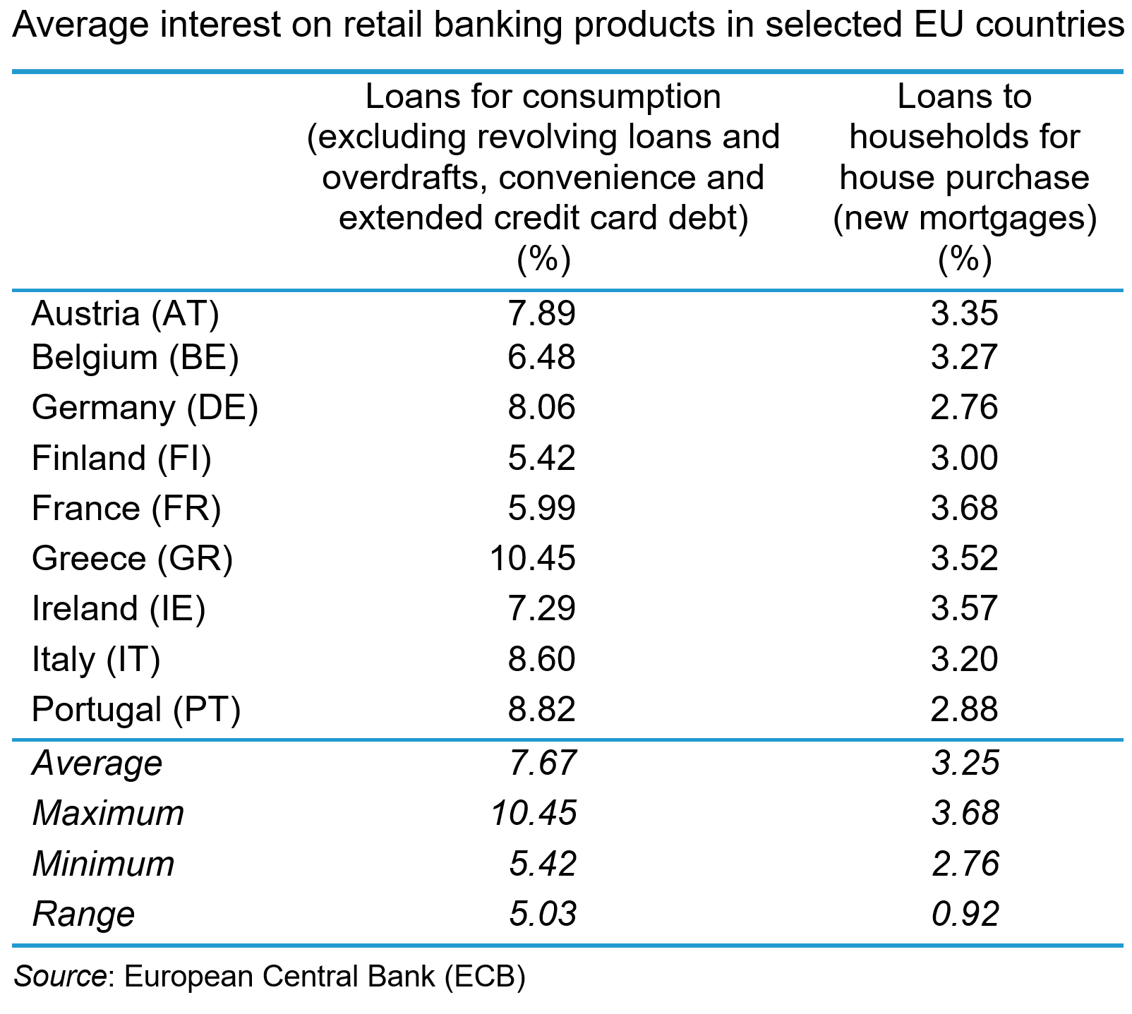
The data show a range of average interest rates offered across the countries with a range of 5.03% for loans to households and 0.92% for new mortgages. These price differentials reflect a broad array of factors, not least the different institutional legal and risk characteristics of the national markets. They also reflect varying degrees of competition and the lack of cross-border trade in retail banking products. Retail banking remains a largely domestic industry within the EU. Cross-border banking services remain a marginal activity with non-domestic retail deposits rising by just 0.5% and non-domestic retail loans rising by just 0.3% between 2016 and 2024.
There are both natural and policy-induced barriers, which means that retail banking will remain largely segmented by nation.
 On the demand-side, retail banking is largely a relational rather than a transactional service, with consumption taking place over a long time-period with significant financial risks attached. Even with deposit insurance and a lender of last resort (the central bank), consumers exhibit significant loss aversion in their use of retail banking services. Consequently, trust and confidence are important characteristics for consumers and that means they are likely to prefer to use familiar domestic institutions.
Further, perceptions about switching costs mean that consumers are reluctant to change suppliers. Such costs are exacerbated by language, cultural and legal differences between European countries, which can make the perceived costs of banking beyond national boundaries prohibitively expensive and create a preference for local institutions.
Consumer preferences can also create idiosyncratic market structures for retail banking services in particular countries. For instance, in several countries across the EU, notably Germany, mutualised credit unions account for significant shares of retail banking. This may limit the potential for foreign banks to penetrate Europe’s largest market.
There are also policy-induced obstacles to cross-border retail banking which operate on the demand-side. These include discriminatory tax treatment of foreign financial services which deters their purchase by consumers. Further, there are still eight different currencies used in the EU across the 27 member states (Denmark, Poland and Sweden are three significant examples). This creates costs and risks associated with currency exchange for consumers that may deter their use of cross-border deposits and loans. The full adoption of a single currency across the EU seems a long way off, which will limit the potential for a single banking market, particularly in the retail segment.
Retail banking as a public utility
 Some argue that retail banking is a public utility and should be regulated as such. It has a simple business model, taking deposits, making payments and making loans. Like other utilities, such as water and energy, retail banking is an essential service for the smooth functioning of the economy and society. Like other utilities, bank failures create severe problems for the economy and society.
Since the financial crisis, stability in retail banking has been much more highly valued. In the period preceding the crisis, banks had used retail deposits to cross-subsidise their risky investment banking. The bank failures that resulted from this had severe economic consequences. The danger today is that by relaxing capital and liquidity restrictions too much, large banks may once again engage in risky behaviour, subsidised by retail banking – for example, by engaging in cross-border M&As. These may benefit their shareholders but provide little benefit to retail customers.
Further, allowing these large banks freedom to move funds around the bloc may lead to capital being concentrated in the most profitable markets, leaving less profitable markets / countries underserved. Retail banking, as a public utility, should be required to provide services there.
Who ultimately benefits?
The integration of banking services in the EU has progressed since the financial crisis, producing a more resilient system. However, there are features of retail banking which mean that integration which benefits consumers may be difficult to achieve.
Addressing the policy gaps identified by the AFME report may benefit large European banks by facilitating the scale economies to make them competitive internationally. However, until consumers are prepared, or able, to source banking services beyond national borders, they will see little benefit from European Banking Union (EBU) through lower prices and/or better service. The nature of retail banking in the EU suggests that this is unlikely any time soon.
Furthermore, since retail banking exhibits features of a public utility, regulators need to be wary of permitting the type of behaviour by large institutions which creates dangerous systemic risk. The worry is that, in the drive to create ‘European Champions’ in banking, regulators ignore the potential impact on retail customers.
Articles
Book
Report
Data and Information
Questions
- Using an average cost (AC) schedule, illustrate the efficiency benefits for large European banks from banking union.
- Analyse the sources of efficiency gains that European banks can gain from cross-border M&As.
- Explain how European retail banking customers could gain from such efficiency.
- Analyse why they may not.
- Analyse whether retail banking in Europe needs to be regulated as a public utility.
 The gold market has become one of the most talked-about commodity markets in 2025, with prices reaching record highs. This is largely due to increased demand from investors, who see gold as a ‘safe haven’ during times of economic and political uncertainty. Central banks are also buying more gold as a way to reduce their reliance on currencies like the US dollar. With many analysts predicting prices could reach over $4000 per ounce in the next year, the gold market is showcasing how supply and demand, confidence, and global events can all influence a commodity market.
The commodities market is where basic agricultural products, raw materials and metals, such as gold, are bought and sold, often in large quantities and across global exchanges. Commodities are typically traded either in their physical form (like gold bars) at current market prices (spot prices) or through financial contracts, where investors buy or sell in futures markets. These are where a price is agreed today to buy or sell on a specific future date.
As with other commodities, the price of gold is determined by supply and demand. Demand for gold typically rises during times of economic uncertainty as investors want a safer store of value. This results in an increase in its price. Supply and demand, and hence price, also respond to other factors, including interest rates, currency movements, economic growth and growth prospects, and geopolitical events.
Record high prices
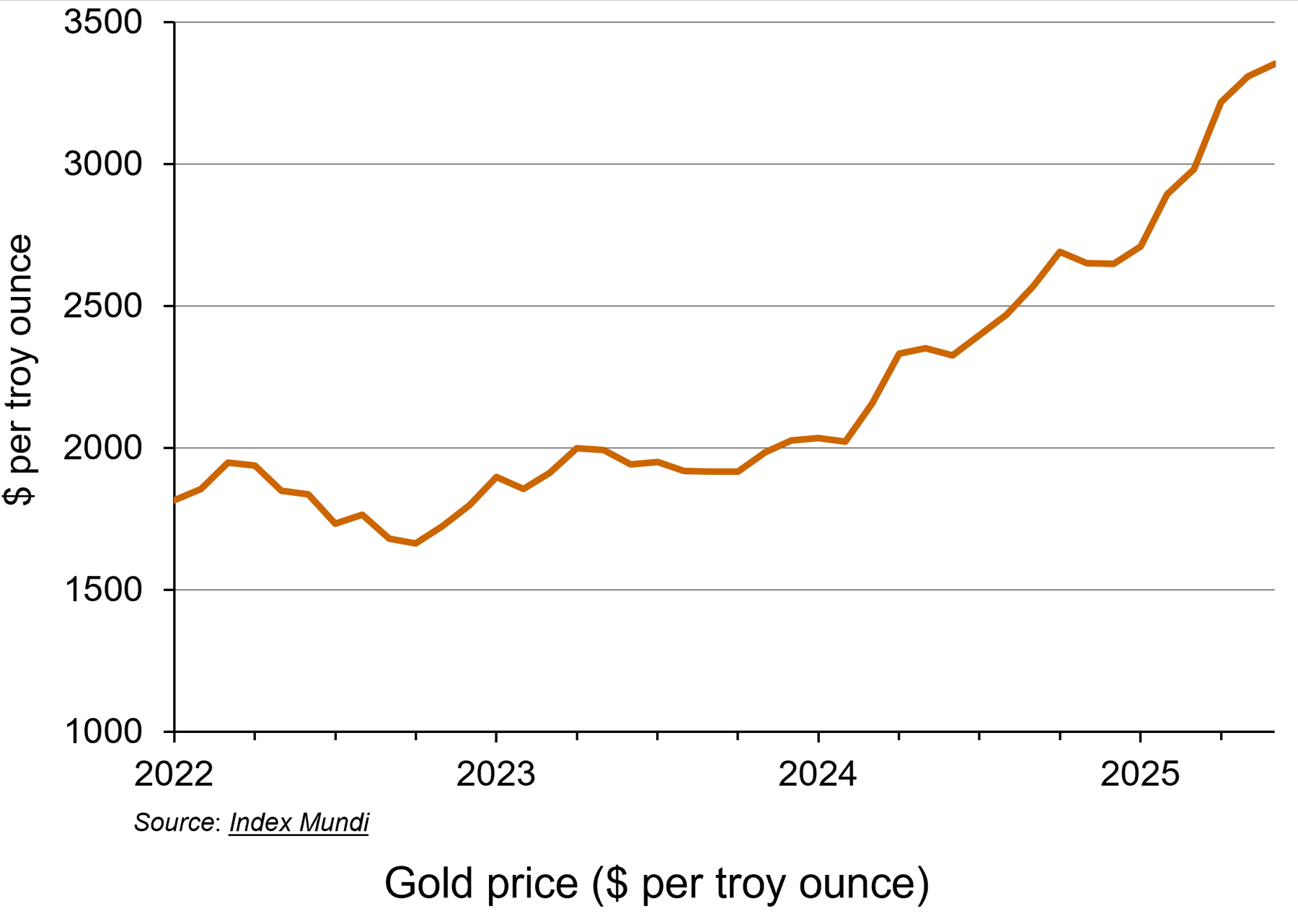 This year, the gold market has seen a remarkable rally, with the price of gold hitting a record high. Demand for the precious metal has resulted in spot prices surging over 35% to date (see the chart: click here for a PowerPoint). Rising prices earlier this year have been attributed to the US President, Donald Trump, announcing wide-ranging tariffs which have upset global trade. On 2 September, the spot gold price hit $3508.50 per ounce, continuing its upwards trend.
The price has also been lifted by expectations that the Federal Reserve (the US central bank) will cut its key interest rate, making gold an even more attractive prospect for investors. If the Federal Reserve cuts interest rates, the price of gold usually increases. This is because gold does not pay any interest or yield, so when interest rates are high, investors can earn better returns from alternatives, such as savings accounts or bonds. However, when interest rates fall, those returns become less attractive, making gold relatively more appealing.
Lower interest rates also tend to weaken the US dollar, which makes gold cheaper for foreign buyers, increasing global demand. Since gold is priced in dollars, a weaker dollar usually leads to higher gold prices.
Additionally, interest rate cuts are often a response to economic problems or uncertainty. As gold is viewed as a safer asset for investors during times of economic uncertainty, investors will typically increase their demand.
Unlike the market for currencies or shares, gold doesn’t rely on the performance of a government or company. This makes it attractive when people are worried about things like inflation, recession, war or stock market crashes. Gold is thus seen as a ‘safe haven’.
Gold and the Federal Reserve
 The rise in the price of gold by more than a third this year can be linked to the US election last year, according to the director of research at BullionVault (see the BBC article below). Attitudes of the Trump administration towards the Federal Reserve have created concerns among investors. Fears that the US administration could erode the independence of the world’s most important central bank have fuelled the latest flows into the metal, which is traditionally viewed as a hedge against inflation.
According to the BBC article, Derren Nathan from Hargreaves Lansdown claims that it is Trump’s ‘attempts to undermine the independence of the Federal Reserve Bank’ that were ‘driving renewed interest in safe haven assets, including gold’. Investors are concerned that a politicised Fed would be more inclined to cut interest rates than would otherwise be the case, sending long-term inflation expectations higher.
This could lead to fears that future interest rates would then be pushed higher. This would increase the yields on longer-term government bonds by pushing down their price, as investors demand higher compensation for the increased risk of higher future interest rates reducing the value of their fixed-rate investments. This would force the US Treasury to pay higher interest on new bonds, making it more expensive to service US government debt.
Expected price rises for 2026
As we saw above, it is predicted that the price of gold will rise to $4000 per ounce next year. However, if the market sees investors move away from dollar assets, such as US Treasuries, the price increases would be even higher. Daan Struyven, co-head of global commodities research at Goldman Sachs explains ‘If 1 per cent of the privately owned US Treasury market were to flow to gold, the gold price would rise to nearly $5000 per troy ounce’ (see Financial Times article below).
 If the Federal Reserve does come under political pressure, it could affect the stability of the US economy and beyond. When gold prices rise sharply, demand usually falls in countries like China and India, which are the world’s largest buyers of gold jewellery. However, in 2025, this trend has changed. Instead of reducing their gold purchases, people in these countries have started buying investment gold, such as bars and coins, showing a shift in consumer behaviour from jewellery to investment assets.
At the same time, global events are also influencing the gold market. Suki Cooper, a metals analyst at Standard Chartered, said that events like Russia’s invasion of Ukraine have added to political uncertainty, which tends to increase demand for gold as a safe-haven asset. She also highlighted how changes in international trade policies have disrupted supply chains and contributed to higher inflation, both of which have made gold more attractive to investors. Additionally, a weaker US dollar earlier in the year made gold cheaper for buyers using other currencies, which boosted global demand even further.
Conclusion
Although the gold market is expected to remain strong over the next six months, some uncertainty remains. Many analysts predict that gold prices will stay high or even increase further, especially if interest rates in the US are cut as expected. Continued global instability, is also likely to keep demand for gold as a safe haven high. At the same time, if inflation stays elevated or trade disruptions continue, more investors may turn to gold to protect their wealth.
However, if economic conditions stabilise or interest rates rise again, gold demand could fall slightly, leading to a potential dip in prices. Overall, the outlook for gold remains positive, but sensitive to changes in global economic and political events.
Articles
- Gold price hits record high as investors seek safety
BBC News, Faarea Masud (2/9/25)
- Safe-haven gold rally gains further momentum after soft US data
Reuters, Sherin Elizabeth Varghese and Ashitha Shivaprasad (3/9/25)
- Gold vaults $3,000 in rush for safety from market, political worry
Reuters, Sherin Elizabeth Varghese and Anmol Choubey (14/3/25)
 The foundation of gold’s rally to historic highs started back in 2022
CNBC, Suki Cooper (17/3/25)
- Gold could hit nearly $5,000 if Trump undermines Fed, says Goldman Sachs
Financial Times, Emily Herbert (4/9/25)
- London’s bullion market set to trial digital gold
City AM, Maisie Grice (3/8/25)
- Gold price hits record high as investors seek safe haven
The Guardian, Julia Kollewe (2/9/25)
Data
Questions
- What factors influence the price of a commodity such as gold on the global market?
- Use a demand and supply diagram to illustrate what has been happening to the gold price in recent months.
- Find out what has been happening to silver prices. Are the explanations for the price changes the same as for gold?
- Why might investors choose to buy gold during times of economic or political uncertainty?
- How will changes in interest rates affect both the demand for and the price of gold?
- What are the possible consequences of rising gold prices for countries like India and China, where there is a traditionally high demand for gold jewellery?
- How do global events impact commodity markets? Use gold as an example in your answer.
 On 25 October 2024, Moody’s, one of the major credit ratings agencies, announced that it was downgrading France’s economic outlook to negative. This was its first downgrading of France since 2012. It followed a similar revision by Fitch’s, another ratings agency, on 11 October.
While Fitch’s announcement did not have a significant impact on the yields of French government bonds, expectations around Moody’s did. In the week preceding the announcement, the net increases in the yield on generic 10-year government debt was approximately 9 basis points (0.09 percentage points). On the day itself, the yield rose by approximately 5.6 basis points (0.056 percentage points).
The yield rose further throughout the rest of October, finishing nearly 0.25 percentage points above its level at the start of the month. However, as Figure 1 illustrates, these increases are part of a longer-term trend of rising yields for French government debt (click here for a PowerPoint).
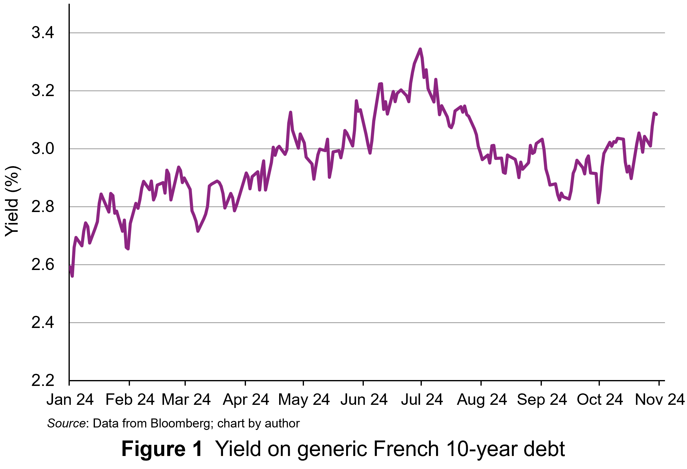 The yield on 10-year French government debt began 2024 at 2.56% and had an upward trend for the first half of the year. The yield peaked at 3.34% on 1 July. It then fell back below 3% for a while. The negative economic outlook then pushed yields back above 3% and they finished October at 3.12%, half a percentage point above the level at the start of the year. This represents a significant increase in borrowing costs for the French government.
In this blog, we will explain why the changes in France’s economic outlook translate into increases in yields for French government bonds. We will also analyse why yields have increased and examine the prospects for the markets in French government bonds.
Pricing signals of bond yields
A bond is a tradable debt instrument issued by governments to finance budget deficits – the difference between tax receipts and spending. Like any financial instruments, investment in bonds involves a commitment of funds today in anticipation of interest payments through time as compensation, with a repayment of its redemption value on the date the bond matures.
Since the cash flows associated with holding a bond occur at different points in time, discounted cash flow analysis is used to determine its value. This gives the present value of the cash flows discounted at the appropriate expected rate of return. In equilibrium this will be equal to the bond’s market price, as the following equation shows.

Where:
P = the equilibrium price of the bond
C = cash coupon payments
M = redemption value at maturity
r = yield (expected rate of return in equilibrium.
Interest payments tend to be fixed at the time a bond is issued and reflect investors’ expected rate of return, expressed as the yield in bond markets. This is determined by prevailing interest rates and perceived risk. Over time, changes in interest rates and perceptions of risk will change the expected rate of return (yield), which will, in turn, change the present value of the cash flows, and hence fundamental value.
Prices move in response to changes in fundamental value and since this happens frequently, this means that prices change a lot. For bonds, as the coupon payments (C each year and the redemption price () are fixed, the only factor that can change is the expected rate of return (yield). This is reflected in the observed yield at each price.
 If the expected rate of return rises, this increases the discount rate applied to future cash flows and reduces their present value. At the current price, the fixed coupon is not sufficient to compensate investors. So, investors sell the bonds and price falls until it reaches a point where the yield offered is equal to that required. The reverse happens if the expected rate of return falls.
The significant risk associated with bonds is credit default risk – the risk that the debt will not be repaid. The potential for credit default is a significant influence of the compensation investors require for holding debt instruments like bonds (ceteris paribus). An increase in expected credit default risk will increase the expected return (compensation). This will be reflected in a lower price and higher yield.
Normally, with the bonds issued by high-income countries, such as those in Europe and North America, the risk of default is extremely low. However, if a country’s annual deficits or accumulated debt increase to what markets consider to be unsustainable levels, the perceived risk of default may rise. Countries’ levels of risk are rated by international ratings agencies, such as Moody’s and Fitch. Investors pay a lot of attention to the information provided by such agencies.
Moody’s downgrade in its economic outlook for France from ‘stable’ to ‘negative’ indicated weak economic performance and higher credit default risk. This revision rippled through bond markets as investors adjusted their views of the country’s economic risk. The rise in yields observed is a signal that bond investors perceive higher credit default risk associated with French government debt and are demanding a higher rates of return as compensation.
Why has France’s credit default risk premium risen now?
As we have seen, credit default risk is not normally considered a significant issue for sovereign borrowers like France. Some of the issue around perceived credit default risk for the French government relate to the size of the French government’s deficit and the projections for it. Following a spike in borrowing associated with the COVID-19 pandemic in 2020, the annual government budget deficit and the overall level of debt as percentages of GDP have remained high. The annual deficit is projected to be 6% for 2024 and still 5% for 2025. The ratio of outstanding French government debt to Gross Domestic Product (GDP) ballooned to 123% in 2020 and is still expected to be 115% by the end of 2025. France has been put on notice to reduce its debt towards the Eurozone limit of 60% of GDP.
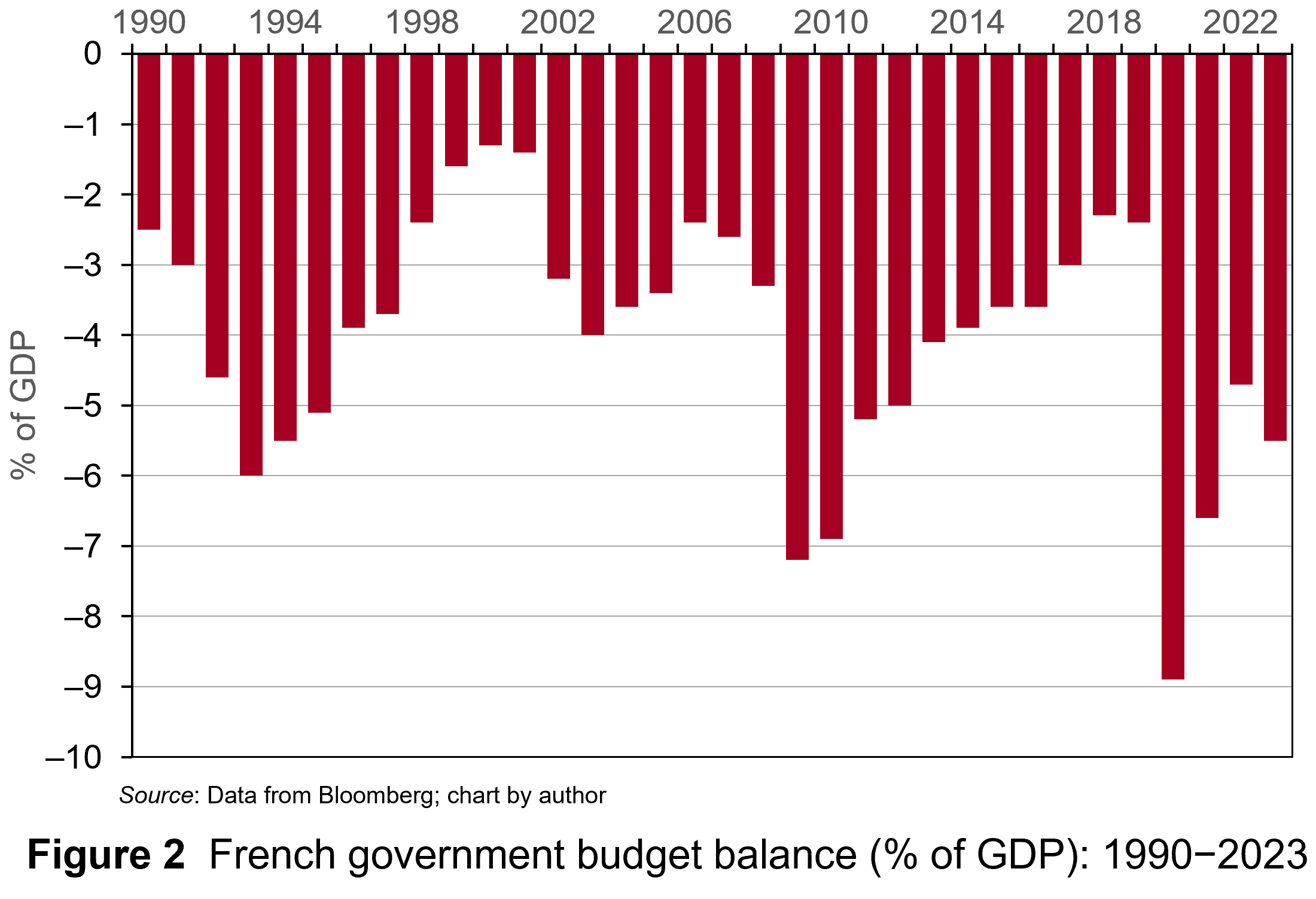 Governments in France last achieved a balanced budget in 1974. They have run deficits ever since. Figure 2 illustrates the French government budget deficits from 1990 to 2023 (click here for a PowerPoint). The figure shows that France experienced deficits in the past similar to today’s. These, however, did not tend to worry bond markets too much.
So why are investors currently worried? This stems from France’s debt mountain and from concerns that the government will not be able to deal with it. Investors are concerned that both weak growth and increasingly volatile politics will thwart efforts to reduce debt levels.
Let’s take growth. Even by contemporary European standards, France’s growth prospects are anaemic. GDP is expected to grow by just 1.1% for 2024 and 1% for 2025. Both consumer and business confidence are low. None of this suggests a growth spurt soon which will boost the tax revenues of the French government sufficiently to address the deficit.
 Further, political instability has grown due to the inconclusive parliamentary elections which Emmanuel Macron surprisingly called in July. No single political grouping has a majority and the President has appointed a Centrist Prime Minister, Michel Barnier (the former EU Brexit negotiator). His government is trying to pass a budget through the Assemblée Nationale involving a mixture of spending cuts and tax hikes which amount to savings of €60 billion ($66 billion). This is equivalent to 2% of GDP.
The parliamentary path of the budget bill is set to be torturous with both the left and right wing blocs in the Assemblée opposing most of the provisions. Debate in the Assemblée Nationale and Senate are expected to drag on into December, with the real prospect that the government may have to use presidential decree to pass the budget. Commentators argue that this will fuel further political chaos.
France looks more like Southern Europe
 In the past, bond investors were more tolerant of France’s budget deficits. French government bonds were attractive options for investors wanting to hold euro-denominated bonds while avoiding riskier Southern European countries such as Greece, Italy, Portugal and Spain. Since France has run persistent government deficits for a long time, it offered bond investors a more liquid market than more fiscally-parsimonious Northern European neighbours, such as Germany and the Netherlands. Consequently, France’s debt instruments offered a slight risk premium on the yields for those countries.
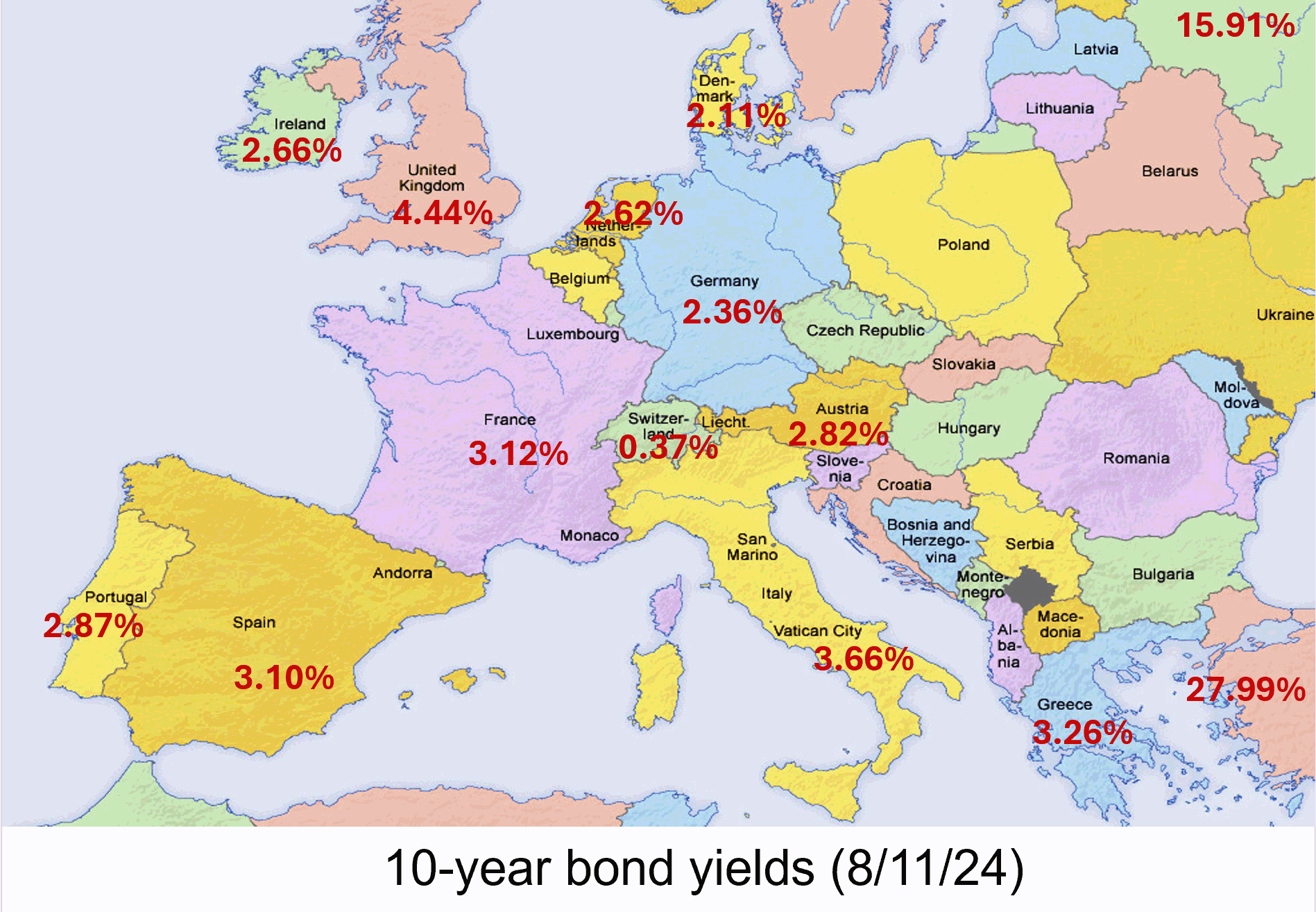
However, that has changed. France’s credit default risk premium is rising to levels comparable to its Southern neighbours. On 26 September 2024, the yield on generic French government 10-year debt rose above its Spanish equivalent for the first time since 2008.
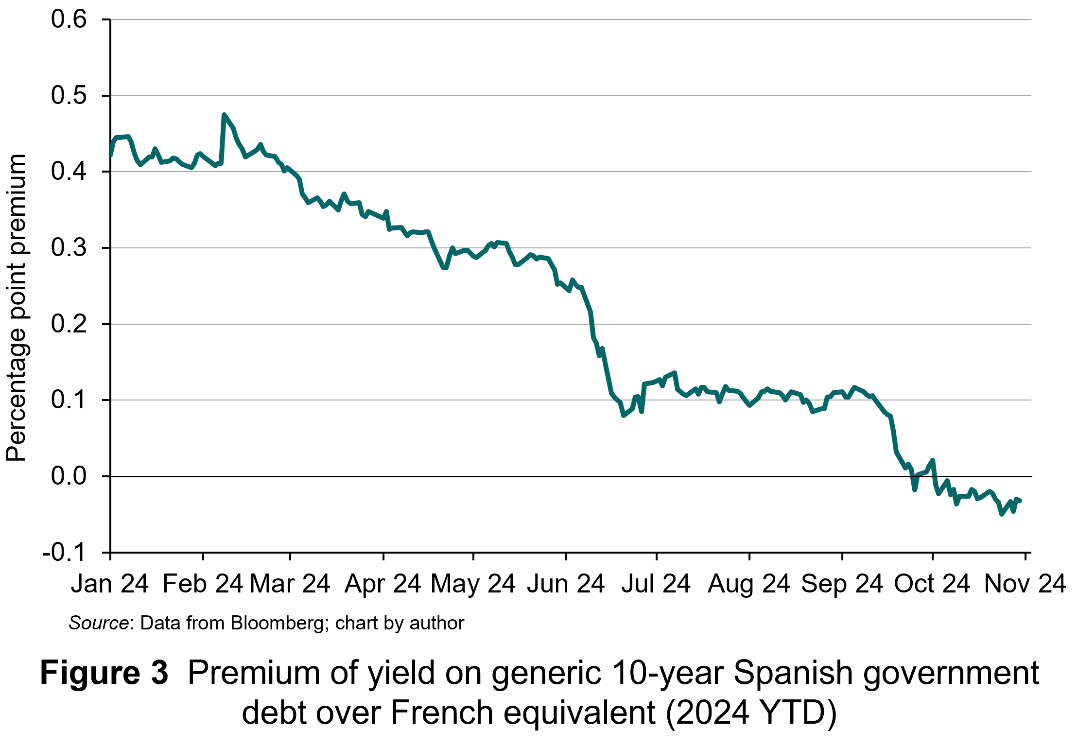 As Figure 3 illustrates, this was the culmination of a trend evident throughout 2024, with the difference in yields between the two declining steadily (click here for a PowerPoint). At the start of the year, the yield on Spanish debt offered a 40 basis points premium over the French equivalent. By October, the yield on Spanish debt was consistently below that of French debt. All of this is due to bond investors’ rising expectations about France’s credit default risk. Now, France’s borrowing costs are not only above Spain, but also closer to those of Greece and Italy than of Germany.
Strikingly, Spain’s budget deficit was 3.5% in 2023 and is expected to narrow to 2.6% by 2025. The percentage of total debt to GDP is 104% and falling. Moreover, following Spain’s inconclusive election in 2023, the caretaker government put forward budgetary plans involving fiscal tightening without the need for legislation. This avoided the political wrangling France is facing.
For France, these developments raise the prospect of yields rising further as bond investors now see alternatives to French government debt in the form of Spain’s. This country have already undertaken the painful fiscal adjustments that France seems incapable of completing.
Articles
Data
Questions
- What is credit default risk?
- Explain why higher credit default risk is associated with higher yields on France’s government debt.
- Why would low economic growth worsen the government’s budget deficit?
- Why would political instability increase credit default risk?
- What has happened to investors’ perceptions of the risk associated with French government debt relative to Spain’s?
- How has this manifested itself in the relative yields of the two countries’ government debt?
 Wobbles in the private credit market in the fourth quarter of 2025 spooked those retail investors with investments in private credit funds – a significant segment of the growing shadow banking sector. These funds use investors’ money to finance lending to businesses and individuals who struggle to, or do not want to, access credit from banks and the public market. Therefore, the risks are higher.
 Such investors are attracted by the potential for higher returns that private credit funds offered compared to public funds. The need to provide higher returns was related partly to the higher credit risk associated with the lending, but also to the illiquidity of the private credit assets that the funds invested in.
  Banks offer maturity transformation by offering current and other accounts to individuals where deposits can be redeemed at short notice. These institutions use the deposits to finance long-term lending for a variety of purposes; examples include property, investment in capital or day-to-day spending. Their effective management of this process is important economically for the smooth running of the payments mechanism and for economic growth.
  Offering liquidity confounds that. To do so, private credit funds end up operating like quasi-public funds. They have to hold sufficient liquid assets to cover redemptions. Indeed, regulations for such funds in Europe are proposing a minimum of 20% of assets in liquid investments so there is a reserve to meet redemptions. But, by doing so, funds will not be able to generate the promised returns. Indeed, returns may be not much higher that that offered by public traded funds.
  Donald Trump is keen to lower US interest rates substantially and rapidly in order to provide a boost to the US economy. He is also keen to reduce the cost of living for US citizens and sees lower interest rates as a means of reducing the burden of debt servicing for both consumers and firms alike.
 The Federal Reserve Board decides on monetary policy and then the Federal Open Market Committee (FOMC) decides how to carry it out. It decides on interest rates and asset sales or purchases. The FOMC meets eight times a year.
  What will happen to the dollar, US bond prices, share prices and US inflation, and what will happen to investment, depends on how people respond to the threat to the Fed’s independence. Initially, there was little response from markets, with investors probably concluding that President Trump is unlikely to be able to sway FOMC members. What is more, several Republican lawmakers have begun criticising the Trump administration’s criminal investigation, making it harder for the President to influence Fed decisions.
 Nevertheless, Donald Trump’s actions could well cause investors to become more worried. Will he try to find other ways to undermine the Fed? Will his actions over Venezuela, Cuba, Greenland and Iran, let alone his policies towards Ukraine and Russia and towards Israel and Gaza, heighten global uncertainty? Will his actions towards Venezuela and his desire to take over Greenland embolden China to attempt to annex Taiwan, and Russia to continue to resist plans to end the war in Ukraine or to make stronger demands?

 Even as the EU moved towards economic and monetary union (EMU) during the 1990s, there was no discussion of integration for the banking industry. However, that changed following the 2008 financial crisis and 2011 eurozone crisis. Both episodes exposed vulnerabilities in the EU banking system which required taxpayer support. It was proposed that deeper integration of the banking sector would ensure its stability and resilience. This stimulated moves towards European Banking Union (EBU), starting with the European Council agreeing its creation in 2012. There are three institutional pillars to the Union:
 On the demand-side, retail banking is largely a relational rather than a transactional service, with consumption taking place over a long time-period with significant financial risks attached. Even with deposit insurance and a lender of last resort (the central bank), consumers exhibit significant loss aversion in their use of retail banking services. Consequently, trust and confidence are important characteristics for consumers and that means they are likely to prefer to use familiar domestic institutions.
  Some argue that retail banking is a public utility and should be regulated as such. It has a simple business model, taking deposits, making payments and making loans. Like other utilities, such as water and energy, retail banking is an essential service for the smooth functioning of the economy and society. Like other utilities, bank failures create severe problems for the economy and society.
  The gold market has become one of the most talked-about commodity markets in 2025, with prices reaching record highs. This is largely due to increased demand from investors, who see gold as a ‘safe haven’ during times of economic and political uncertainty. Central banks are also buying more gold as a way to reduce their reliance on currencies like the US dollar. With many analysts predicting prices could reach over $4000 per ounce in the next year, the gold market is showcasing how supply and demand, confidence, and global events can all influence a commodity market.
 This year, the gold market has seen a remarkable rally, with the price of gold hitting a record high. Demand for the precious metal has resulted in spot prices surging over 35% to date (see the chart: click
  If the Federal Reserve does come under political pressure, it could affect the stability of the US economy and beyond. When gold prices rise sharply, demand usually falls in countries like China and India, which are the world’s largest buyers of gold jewellery. However, in 2025, this trend has changed. Instead of reducing their gold purchases, people in these countries have started buying investment gold, such as bars and coins, showing a shift in consumer behaviour from jewellery to investment assets.
 On 25 October 2024, Moody’s, one of the major credit ratings agencies, announced that it was downgrading France’s economic outlook to negative. This was its first downgrading of France since 2012. It followed a similar revision by Fitch’s, another ratings agency, on 11 October.
 The yield on 10-year French government debt began 2024 at 2.56% and had an upward trend for the first half of the year. The yield peaked at 3.34% on 1 July. It then fell back below 3% for a while. The negative economic outlook then pushed yields back above 3% and they finished October at 3.12%, half a percentage point above the level at the start of the year. This represents a significant increase in borrowing costs for the French government.
 Governments in France last achieved a balanced budget in 1974. They have run deficits ever since. Figure 2 illustrates the French government budget deficits from 1990 to 2023 (click
  Further, political instability has grown due to the inconclusive parliamentary elections which Emmanuel Macron surprisingly called in July. No single political grouping has a majority and the President has appointed a Centrist Prime Minister, Michel Barnier (the former EU Brexit negotiator). His government is trying to pass a budget through the Assemblée Nationale involving a mixture of spending cuts and tax hikes which amount to savings of €60 billion ($66 billion). This is equivalent to 2% of GDP.
 In the past, bond investors were more tolerant of France’s budget deficits. French government bonds were attractive options for investors wanting to hold euro-denominated bonds while avoiding riskier Southern European countries such as Greece, Italy, Portugal and Spain. Since France has run persistent government deficits for a long time, it offered bond investors a more liquid market than more fiscally-parsimonious Northern European neighbours, such as Germany and the Netherlands. Consequently, France’s debt instruments offered a slight risk premium on the yields for those countries.
  As Figure 3 illustrates, this was the culmination of a trend evident throughout 2024, with the difference in yields between the two declining steadily (click