Bubbles
 Speculation in markets can lead to wild swings in prices as exuberance drives up prices and
pessimism leads to price crashes. When the rise in price exceeds underlying fundamentals, such as profit, the result is a bubble. And bubbles burst.
There have been many examples of bubbles throughout history. One of the most famous is that of tulips in the 17th century. As Box 2.4 in Essential Economics for Business (6th edition) explains:
Between November 1636 and February 1637, there was a 20-fold increase in the price of tulip bulbs, such that a skilled worker’s annual salary would not even cover the price of one bulb. Some were even worth more than a luxury home! But, only three months later, their price had fallen by 99 per cent. Some traders refused to pay the high price and others began to sell their tulips. Prices began falling. This dampened demand (as tulips were seen to be a poor investment) and encouraged more people to sell their tulips. Soon the price was in freefall, with everyone selling. The bubble had burst .
Another example was the South Sea Bubble of 1720. Here, shares in the South Sea Company, given a monopoly by the British government to trade with South America, increased by 900% before collapsing through a lack of trade.
Another, more recent, example is that of Poseidon. This was an Australian nickel mining company which announced in September 1969 that it had discovered a large seam of nickel at Mount Windarra, WA. What followed was a bubble. The share price rose from $0.80 in mid-1969 to a peak of $280 in February 1970 and then crashed to just a few dollars.
Other examples are the Dotcom bubble of the 1990s, the US housing bubble of the mid-2000s and BitCoin, which has seen more than one bubble.
Bubbles always burst eventually. If you buy at a low price and sell at the peak, you can make a lot of money. But many will get their fingers burnt. Those who come late into the market may pay a high price and, if they are slow to sell, can then make a large loss.
GameStop shares – an unlikely candidate for a bubble
 The most recent example of a bubble is GameStop. This is a chain of shops in the USA selling games, consoles and other electronic items. During the pandemic it has struggled, as games consumers have turned to online sellers of consoles and online games. It has been forced to close a number of stores. In July 2020, its share price was around $4. With the general recovery in stock markets, this drifted upwards to just under $20 by 12 January 2021.
Then the bubble began.
Hedge fund shorting
Believing that the GameStop shares were now overvalued and likely to fall, many hedge funds started shorting the shares. Shorting (or ‘short selling’) is where investors borrow shares for a fee and immediately sell them on at the current price, agreeing to return them to the lender on a specified day in the near future (the ‘expiration date’). But as the investors have sold the shares they borrowed, they must now buy them at the current price on or before the expiration date so they can return them to the lenders. If the price falls between the two dates, the investors will gain. For example, if you borrow shares and immediately sell them at a current price of £5 and then by the expiration date the price has fallen to $2 and you buy them back at that price to return them to the lender, you make a £3 profit.
But this is a risky strategy. If the price rises between the two dates, investors will lose – as events were to prove.
The swarm of small investors
 Enter the ‘armchair investor’. During lockdown, small-scale amateur investing in shares has become a popular activity, with people seeking to make easy gains from the comfort of their own homes. This has been facilitated by online trading platforms such as Robinhood and Trading212. These are easy and cheap, or even free, to use.
What is more, many users of these sites were also collaborating on social media platforms, such as Reddit. They were encouraging each other to buy shares in GameStop and some other companies. In fact, many of these small investors were seeing it as a battle with large-scale institutional investors, such as hedge funds – a David vs. Goliath battle.
With swarms of small investors buying GameStop, its share price surged. From $20 on 12 January, it doubled in price within two days and had reached $77 by 25 January. The frenzy on Reddit then really gathered pace. The share price peaked at $468 early on 28 January. It then fell to $126 less than two hours later, only to rise again to $354 at the beginning of the next day.
Many large investors who had shorted GameStop shares made big losses. Analytics firm Ortex estimated that hedge funds lost a total of $12.5 billion in January. Many small investors, however, who bought early and sold at the peak made huge gains. Other small investors who got the timing wrong made large losses.
And it was not just GameStop. Social media were buzzing with suggestions about buying shares in other poorly performing companies that large-scale institutional investors were shorting. Another target was silver and silver mines. At one point, silver prices rose by more than 10% on 1 February. However, money invested in silver is huge relative to GameStop and hence small investors were unlikely to shift prices by anything like as much as GameStop shares.
Amidst this turmoil, the US Securities and Exchange Commission (SEC) issued a statement on 29 January. It warned that it was working closely with other regulators and the US stock exchange ‘to ensure that regulated entities uphold their obligations to protect investors and to identify and pursue potential wrongdoing’. It remains to be seen, however, what it can do to curb the concerted activities of small investors. Perhaps, only the experience of bubbles bursting and the severe losses that can result will make small investors think twice about backing failing companies. Some Davids may beat Goliath; others will be defeated.
Articles
- GameStop: The competing forces trading blows over lowly gaming retaile
Sky News (30/1/21)
- Tempted to join the GameStop ‘angry mob’? Lessons on bubbles, market abuse and stock picking from the investment experts… including perma-bear Albert Edwards
This is Money, Tanya Jefferies (29/1/21)
- A year ago on Reddit I suggested investing in GameStop. But I never expected this
The Guardian, Desmund Delaney (29/1/21)
- The real lesson of the GameStop story is the power of the swarm
The Guardian, Brett Scott (30/1/21)
- GameStop: What is it and why is it trending?
BBC News, Kirsty Grant (29/1/21)
- GameStop: Global watchdogs sound alarm as shares frenzy grows
BBC News (30/1/21)
- The GameStop affair is like tulip mania on steroids
The Guardian, Dan Davies (29/1/21)
- GameStop news: Short sellers lose $19bn as Omar says billionaires who pressured apps should go to jail
Independent, Andy Gregory, Graig Graziosi and Justin Vallejo (30/1/21)
- Robinhood tightens GameStop trading curbs again as SEC weighs in
Financial Times, Michael Mackenzie, Colby Smith, Kiran Stacey and Miles Kruppa (29/1/21)
- SEC Issues Vague Threats Against Everyone Involved in the GameStop Stock Saga
Gizmodo, Andrew Couts (29/1/21)
- SEC warns it is monitoring trade after GameStop surge
RTE News (29/1/21)
- GameStop short-squeeze losses at $12.5 billion YTD – Ortex data
Reuters (1/2/21)
- GameStop: I’m one of the WallStreetBets ‘degenerates’ – here’s why retail trading craze is just getting started
The Conversation, Mohammad Rajjaque (3/2/21)
- What the GameStop games really mean
Shares Magazine, Russ Mould (4/2/21)
Data
Questions
- Distinguish between stabilising and destabilising speculation.
- Use a demand and supply diagram to illustrate destabilising speculation.
- Explain how short selling contributed to the financial crisis of 2007/8 (see Box 2.7 in Economics (10th edition) or Box 3.4 in Essentials of Economics (8th edition)).
- Why won’t shares such as GameStop go on rising rapidly in price for ever? What limits the rise?
- Find out some other shares that have been trending among small investors. Why were these specific shares targeted?
- How has quantitative easing impacted on stock markets? What might be the effect of a winding down of QE or even the use of quantitative tightening?
 The BBC podcast linked below looks at the use of quantitative easing since 2009 and especially the most recent round since the onset of the pandemic.
Although QE was a major contributor to reducing the depth of the recession in 2009–10, it was barely used from 2013 to 2020 (except for a short period in late 2016/early 2017). The Coalition and Conservative governments were keen to get the deficit down. In justifying pay restraint and curbing government expenditure, Prime Ministers David Cameron and Theresa May both argued that there ‘was no magic money tree’.
But with the severely dampening effect of the lockdown measures from March 2020, the government embarked on a large round of expenditure, including the furlough scheme and support for businesses.
 The resulting rise in the budget deficit was accompanied by a new round of QE from the beginning of April. The stock of assets purchased by the Bank of England rose from £445 billion (the approximate level it had been since March 2017) to £740 billion by December 2020 and is planned to reach £895 billion by the end of 2021.
So with the effective funding of the government’s deficits by the creation of new money, does this mean that there is indeed a ‘magic money tree’ or, indeed, a ‘magic money forest’? And if so, is it desirable? Is it simply stoking up problems for the future? Or will, as modern monetary theorists maintain, the extra money, if carefully spent, lead to faster growth and a reducing deficit, with low interest rates making it easy to service the debt?
The podcast explores these issues. There is then a longer list of questions than normal relating to the topics raised in the podcast.
Podcast
Questions
- Which of the following are stocks and which are flows?
(a) Money
(b) Income
(c) The total amount people save each month
(d) The money held in savings accounts
(e) Public-sector net debt
(f) Public-sector net borrowing
(g) National income
(h) Injections into the circular flow of income
(i) Aggregate demand
(j) Wealth
- How do banks create money?
- What is the role of the Debt Management Office in the sale of gilts?
- Describe the birth of QE.
- Is raising asset prices the best means of stimulating the economy? What are the disadvantages of this form of monetary expansion?
- What are the possible exit routes from QE and what problems could occur from reducing the central bank’s stock of assets?
- Is the use of QE in the current Covid-19 crisis directly related to fiscal policy? Or is this use of monetary policy simply a means of hitting the inflation target?
- What are the disadvantages of having interest rates at ultra-low levels?
- Does it matter if the stock of government debt rises substantially if the gilts are at ultra-low fixed interest rates?
- What are the intergenerational effects of substantial QE? Does it depend on how debt is financed?
- How do the policy recommendations of modern monetary theorists differ from those of more conventional macroeconomists?
- In an era of ultra-low interest rates, does fiscal policy have a greater role to play than monetary policy?
 On 25 November, the UK government published its Spending Review 2020. This gives details of estimated government expenditure for the current financial year, 2020/21, and plans for government expenditure and the likely totals for 2021/22.
The focus of the Review is specifically on the effects of and responses to the coronavirus pandemic. It does not consider the effects of Brexit, with or without a trade deal, or plans for taxation. The Review is based on forecasts by the Office for Budget Responsibility (OBR). Because of the high degree of uncertainty over the spread of the disease and the timing and efficacy of vaccines, the OBR gives three forecast values for most variables – pessimistic, central and optimistic.
 According to the central forecast, real GDP is set to decline by 11.3% in 2020, the largest one-year fall since the Great Frost of 1709. The economy is then set to ‘bounce back’ (somewhat), with GDP rising by 5.2% in 2021.
Unemployment will rise from 3.9% in 2019 to a peak of 7.5% in mid-2021, after the furlough scheme and other support for employers is withdrawn.
This blog focuses at the impact on government borrowing and debt and the implications for the future – both the funding of the debt and ways of reducing it.
Soaring government deficits and debt
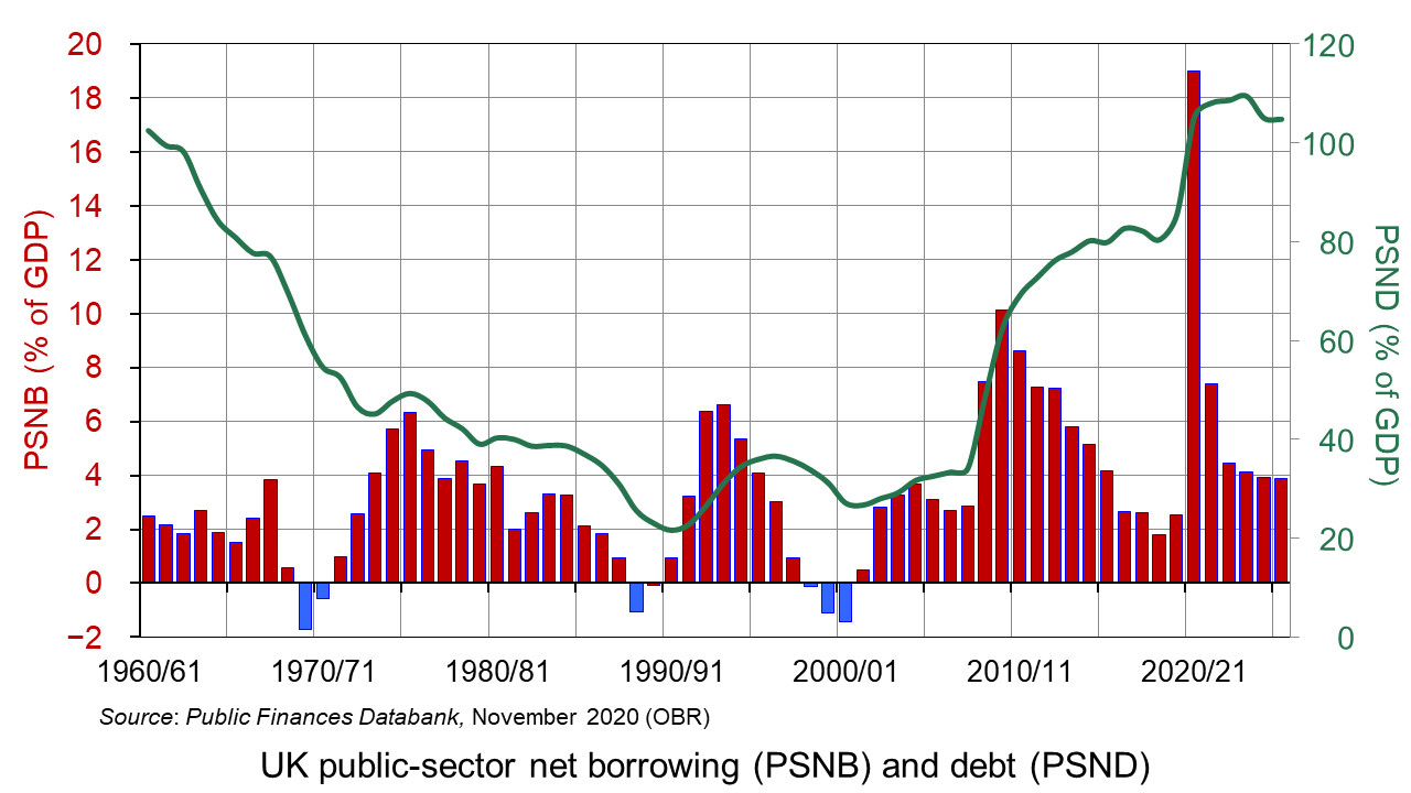
Government expenditure during the pandemic has risen sharply through measures such as the furlough scheme, the Self-Employment Income Support Scheme and various business loans. This, combined with falling tax revenue, as incomes and consumer expenditure have declined, has led to a rise in public-sector net borrowing (PSNB) from 2.5% of GDP in 2019/20 to a central forecast of 19% for 2020/21 – the largest since World War II. By 2025/26 it is still forecast to be 3.9% of GDP. The figure has also been pushed up by a fall in nominal GDP for 2020/21 (the denominator) by nearly 7%. (Click here for a PowerPoint of the above chart.)
The high levels of PSNB are pushing up public-sector net debt (PSNB). This is forecast to rise from 85.5% of GDP in 2019/20 to 105.2% in 2020/21, peaking at 109.4% in 2023/24.
The exceptionally high deficit and debt levels will mean that the government misses by a very large margin its three borrowing and debt targets set out in the latest (Autumn 2016) ‘Charter for Budget Responsibility‘. These are:
- to reduce cyclically-adjusted public-sector net borrowing to below 2% of GDP by 2020/21;
- for public-sector net debt as a percentage of GDP to be falling in 2020/21;
- for overall borrowing to be zero or in surplus by 2025/26.
But, as the Chancellor said in presenting the Review:
Our health emergency is not yet over. And our economic emergency has only just begun. So our immediate priority is to protect people’s lives and livelihoods.
Putting the public finances on a sustainable footing
Running a large budget deficit in an emergency is an essential policy for dealing with the massive decline in aggregate demand and for supporting those who have, or otherwise would have, lost their jobs. But what of the longer-term implications? What are the options for dealing with the high levels of debt?
1. Raising taxes. This tends to be the preferred approach of those on the left, who want to protect or improve public services. For them, the use of higher progressive taxes, such as income tax, or corporation tax or capital gains tax, are a means of funding such services and of providing support for those on lower incomes. There has been much discussion of the possibility of finding a way of taxing large tech companies, which are able to avoid taxes by declaring very low profits by diverting them to tax havens.
2. Cutting government expenditure. This is the traditional preference of those on the right, who prefer to cut the overall size of the state and thus allow for lower taxes. However, this is difficult to do without cutting vital services.  Indeed, there is pressure to have higher government expenditure over the longer term to finance infrastructure investment – something supported by the Conservative government.
A downside of either of the above is that they squeeze aggregate demand and hence may slow the recovery. There was much discussion after the financial crisis over whether ‘austerity policies’ hindered the recovery and whether they created negative supply-side effects by dampening investment.
3. Accepting higher levels of debt into the longer term. This is a possible response as long as interest rates remain at record low levels. With depressed demand, loose monetary policy may be sustainable over a number of years. Quantitative easing depresses bond yields and makes it cheaper for governments to finance borrowing. Servicing high levels of debt may be quite affordable.
The problem is if inflation begins to rise. Even with lower aggregate demand, if aggregate supply has fallen faster because of bankruptcies and lack of investment, there may be upward pressure on prices. The Bank of England may have to raise interest rates, making it more expensive for the government to service its debts.
Another problem with not reducing the debt is that if another emergency occurs in the future, there will be less scope for further borrowing to support the economy.
 4. Higher growth ‘deals’ with the deficit and reduces debt. In this scenario, austerity would be unnecessary. This is the ‘golden’ scenario – for the country to grow its way out of the problem. Higher output and incomes leads to higher tax revenues, and lower unemployment leads to lower expenditure on unemployment benefits. The crucial question is the relationship between aggregate demand and supply. For growth to be sustainable and shrink the debt/GDP ratio, aggregate demand must expand steadily in line with the growth in aggregate supply. The faster aggregate supply can grow, the faster can aggregate demand. In other words, the faster the growth in potential GDP, the faster can be the sustainable rate of growth of actual GDP and the faster can the debt/GDP ratio shrink.
One of the key issues is the degree of economic ‘scarring’ from the pandemic and the associated restrictions on economic activity. The bigger the decline in potential output from the closure of firms and the greater the deskilling of workers who have been laid off, the harder it will be for the economy to recover and the longer high deficits are likely to persist.
Another issue is the lack of labour productivity growth in the UK in recent years. If labour productivity does not increase, this will severely restrict the growth in potential output. Focusing on training and examining incentives, work practices and pay structures are necessary if productivity is to rise significantly. So too is finding ways to encourage firms to increase investment in new technologies.
Podcast and videos
Articles
- Initial reaction from IFS researchers on Spending Review 2020 and OBR forecasts
IFS Press Release, Paul Johnson, Carl Emmerson, Ben Zaranko, Tom Waters and Isabel Stockton (25/11/200
- Rishi Sunak is likely to increase spending – which means tax rises will follow
IFS, Newspaper Article, Paul Johnson (23/11/20)
- Economic and Fiscal Outlook Executive Summary
OBR (25/11/20)
- UK’s Sunak says public finances are on ‘unsustainable’ path
Reuters, David Milliken (26/11/20)
- Rishi Sunak warns ‘economic emergency has only just begun’
BBC News, Szu Ping Chan (25/11/20)
- UK will need £27bn of spending cuts or tax rises, watchdog warns
The Guardian, Phillip Inman (25/11/20)
- What is tomorrow’s Spending Review all about?
The Institute of Chartered Accountants in England and Wales (24/11/20)
- Spending Review 2020: the experts react
The Conversation, Drew Woodhouse, Ernestine Gheyoh Ndzi, Jonquil Lowe, Anupam Nanda, Alex de Ruyter and Simon J. Smith (25/11/20)
OBR Data
Questions
- What is the significance of the relationship between the rate of economic growth and the rate of interest for financing public-sector debt over the longer term?
- What can the government do to encourage investment in the economy?
- Using OBR data, find out what has happened to the output gap over the past few years and what is forecast to happen to it over the next five years. Explain the significance of the figures.
- Distinguish between demand-side and supply-side policies. How would you characterise the policies to tackle public-sector net debt in terms of this distinction? Do the policies have a mixture of demand- and supply-side effects?
- Choose two other developed countries. Examine how their their public finances have been affected by the coronavirus pandemic and the policies they are adopting to tackle the economic effects of the pandemic.
 With the imposition of a new lockdown in England from 5 November to 2 December and in Wales from 3 October to 9 November, and with strong restrictions in Scotland and Northern Ireland, the UK economy is set to return to negative growth – a W-shaped GDP growth curve.
With the closure of leisure facilities and non-essential shops in England and Wales, spending is likely to fall. Without support, many businesses would fail and potential output would fall. In terms of aggregate demand and supply, both would decline, as the diagram below illustrates. (Click here for a PowerPoint.)
The aggregate demand curve shifts from AD1 to AD2 as consumption and investment fall. Exports also fall as demand is hit by the pandemic in other countries. 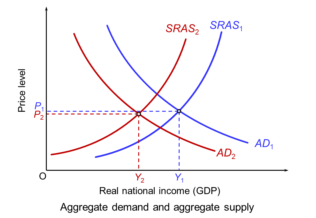 The fall in aggregate supply is represented partly by a movement along the short-run aggregate supply curve (SRAS) as demand falls for businesses which remain open (such as transport services). Largely it is represented by a leftward shift in the curve from SRAS1 to SRAS2 as businesses such as non-essential shops and those in the hospitality and leisure sector are forced to close. What happens to the long-run supply curve depends on the extent to which businesses reopen when the lockdown and any other subsequent restrictions preventing their reopening are over. It also depends on the extent to which other firms spring up or existing firms grow to replace the business of those that have closed. The continuing rise in online retailing is an example.
With the prospect of falling GDP and rising unemployment, the UK government and the Bank of England have responded by giving a fiscal and monetary boost. We examine each in turn.
Fiscal policy
 In March, the Chancellor introduced the furlough scheme, whereby employees temporarily laid off would receive 80% of their wages through a government grant to their employers. This scheme was due to end on 31 October, to be replaced by the less generous Job Support Scheme (see the blog, The new UK Job Support Scheme: how much will it slow the rise in unemployment?). However, the Chancellor first announced that the original furlough scheme would be extended until 2 December for England and then, on 5 November, to the end of March 2021 for the whole of the UK. He also announced that the self-employed income support grant would increase from 55% to 80% of average profits up to £7500.
In addition, the government announced cash grants of up to £3000 per month for businesses which are closed (worth more than £1 billion per month), extra money to local authorities to support businesses and an extension of existing loan schemes for business. Furthermore, the government is extending the scheme whereby people can claim a repayment ‘holiday’ for up to 6 months for mortgages, personal loans and car finance.
The government hopes that the boost to aggregate demand will help to slow, or even reverse, the predicted decline in GDP. What is more, by people being put on furlough rather than being laid off, it hopes to slow the rise in unemployment.
Monetary policy
At the meeting of the Bank of England’s Monetary Policy Committee on 4 November, further expansionary monetary policy was announced. Rather than lowering Bank Rate from its current historically low rate of 0.1%, perhaps to a negative figure, it was decided to engage in further quantitative easing.
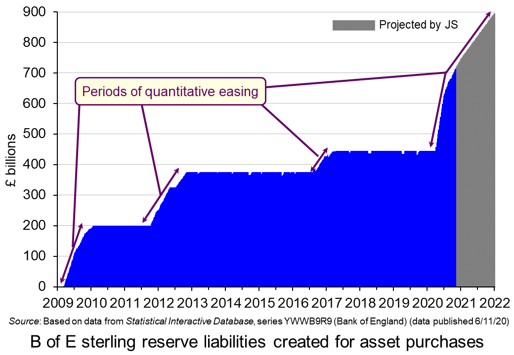 An additional £150 billion of government bonds will be purchased under the asset purchase facility (APF). This will bring the total vale of bonds purchased since the start of the pandemic to £450 billion (including £20 billion of corporate bonds) and to £895 billion since 2009 when QE was first introduced in response to the recession following the financial crisis of 2007–8.
The existing programme of asset purchases should be complete by the end of December this year. The Bank of England expects the additional £150 billion of purchases to begin in January 2021 and be completed within a year.
UK quantitative easing since the first round in March 2009 is shown in the chart above. The reserve liabilities represent the newly created money for the purchase of assets under the APF programme. (There are approximately £30 billion of other reserve liabilities outside the APF programme.) The grey area shows projected reserve liabilities to the end of the newly announced programme of purchases, by which time, as stated above, the total will be £895 billion. This, of course, assumes that the Bank does not announce any further QE, which it could well do if the recovery falters.
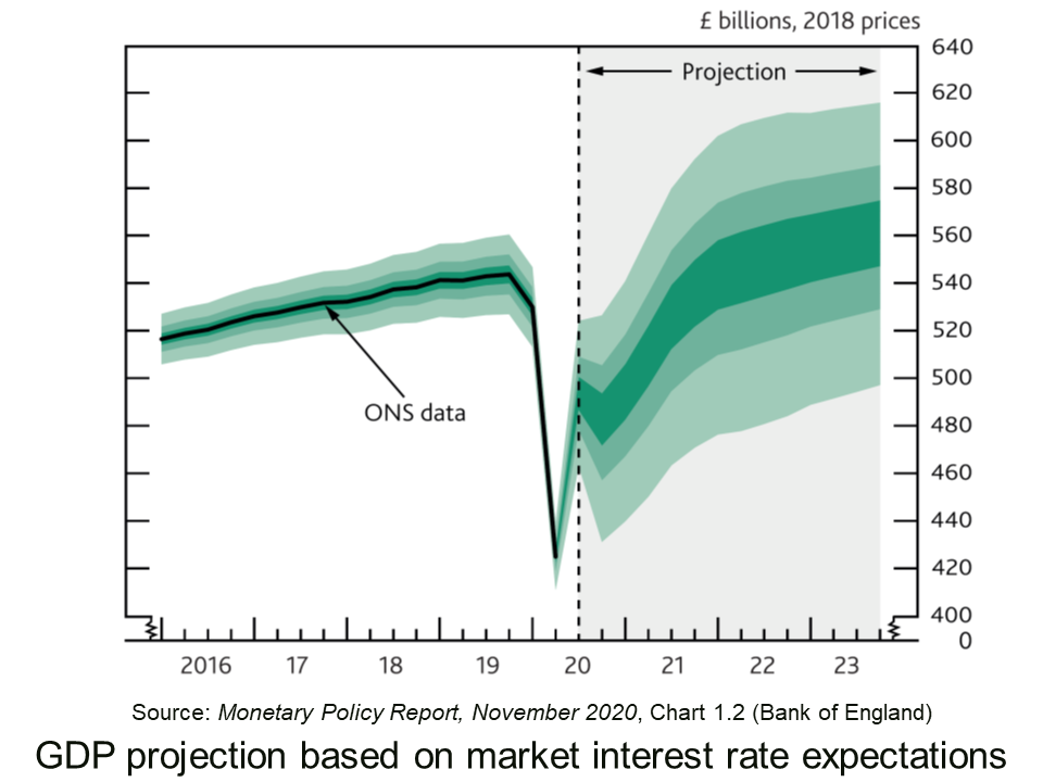
Justifying the decision, the MPC meeting’s minutes state that:
There are signs that consumer spending has softened across a range of high-frequency indicators, while investment intentions have remained weak. …The fall in activity over 2020 has reflected a decline in both demand and supply. Overall, there is judged to be a material amount of spare capacity in the economy.
Conclusions
How effective these fiscal and monetary policy measures will be in mitigating the effects of the Covid restrictions remains to be seen. A lot will depend on how successful the lockdown and other restrictions are in slowing the virus, how quickly a vaccine is developed and deployed, whether a Brexit deal is secured, and the confidence of both consumers, businesses and financial markets that the economy will bounce back in 2021. As the MPC’s minutes state:
The outlook for the economy remains unusually uncertain. It depends on the evolution of the pandemic and measures taken to protect public health, as well as the nature of, and transition to, the new trading arrangements between the European Union and the United Kingdom. It also depends on the responses of households, businesses and financial markets to these developments.
Articles
- Covid: Rishi Sunak to extend furlough scheme to end of March
BBC News (6/11/20)
- Furlough extended until March and self-employed support boosted again
MSE News, Callum Mason (6/11/20)
- Number on furlough in UK may double during England lockdown
The Guardian, Richard Partington (3/11/20)
- ‘We wouldn’t manage without it’: business owners on the furlough extension
The Guardian, Molly Blackall and Mattha Busby (6/11/20)
- Sunak’s abrupt turn on UK furlough scheme draws criticism from sceptics
Financial Times, Delphine Strauss (6/11/20)
 Coronavirus: Bank of England unleashes further £150bn of support for economy
Sky News, James Sillars (5/11/20)
- Bank of England boss pledges to do ‘everything we can’
BBC News, Szu Ping Chan (6/11/20)
- Savers are spared negative rates but the magic money tree delivers £150bn more QE: What the Bank of England’s charts tell us about the economy
This is Money, Simon Lambert (5/11/20)
- Covid-19 and the victory of quantitative easing
The Spectator, Bruce Anderson (26/10/20)
- Will the Bank of England’s reliance on quantitative easing work for the UK economy?
The Conversation, Ghulam Sorwar (9/11/20)
- With a W-shaped recession looming and debt piling up, the government should start issuing GDP-linked bonds
LSE British Politics and Policy blogs, Costas Milas (6/11/20)
Official documents
Questions
- Illustrate the effects of expansionary fiscal and monetary policy on (a) a short-run aggregate supply and demand diagram; (b) a long-run aggregate supply and demand diagram.
- In the context of the fiscal and monetary policy measures examined in this blog, what will determine the amount that the curves shift?
- Illustrate on a Keynesian 45° line diagram the effects of (a) the lockdown and (b) the fiscal and monetary policy measures adopted by the government and Bank of England.
- If people move from full-time to part-time working, how is this reflected in the unemployment statistics? What is this type of unemployment called?
- How does quantitative easing through asset purchases work through the economy to affect output and employment? In other words, what is the transmission mechanism of the policy?
- What determines the effectiveness of quantitative easing?
- Under what circumstances will increasing the money supply affect (a) real output and (b) prices alone?
- Why might quantitative easing benefit the rich more than the poor?
- How could the government use quantitative easing to finance its budget deficit?
 In the current environment of low inflation and rising unemployment, the Federal Reserve Bank, the USA’s central bank, has amended its monetary targets. The new measures were announced by the Fed chair, Jay Powell, in a speech for the annual Jackson Hole central bankers’ symposium (this year conducted online on August 27 and 28). The symposium was an opportunity for central bankers to reflect on their responses to the coronavirus pandemic and to consider what changes might need to be made to their monetary policy targets and instruments.
The Fed’s previous targets
Previously, like most other central banks, the Fed had a long-run inflation target of 2%. It did, however, also seek to ‘maximise employment’. In practice, this meant seeking to achieve a ‘normal’ rate of unemployment, which the Fed regards as ranging from 3.5 to 4.7% with a median value of 4.1%. The description of its objectives stated that:
In setting monetary policy, the Committee seeks to mitigate deviations of inflation from its longer-run goal and deviations of employment from the Committee’s assessments of its maximum level. These objectives are generally complementary. However, under circumstances in which the Committee judges that the objectives are not complementary, it follows a balanced approach in promoting them, taking into account the magnitude of the deviations and the potentially different time horizons over which employment and inflation are projected to return to levels judged consistent with its mandate.
The new targets
 Under the new system, the Fed has softened its inflation target. It will still be 2% over the longer term, but it will be regarded as an average, rather than a firm target. The Fed will be willing to see inflation above 2% for longer than previously before raising interest rates if this is felt necessary for the economy to recover and to achieve its long-run potential economic growth rate. Fed chair, Jay Powell, in a speech on 27 August said:
Following periods when inflation has been running below 2%, appropriate monetary policy will likely aim to achieve inflation moderately above 2 per cent for some time.
Additionally, the Fed has increased its emphasis on employment. Instead of focusing on deviations from normal employment, the Fed will now focus on the shortfall of employment from its normal level and not be concerned if employment temporarily exceeds its normal level. As Powell said:
Going forward, employment can run at or above real-time estimates of its maximum level without causing concern, unless accompanied by signs of unwanted increases in inflation or the emergence of other risks that could impede the attainment of our goals
 The Fed will also take account of the distribution of employment and pay more attention to achieving a strong labour market in low-income and disadvantaged communities. However, apart from the benefits to such communities from a generally strong labour market, it is not clear how the Fed could focus on disadvantaged communities through the instruments it has at its disposal – interest rate changes and quantitative easing.
Assessment
Modern monetary theorists (see blog MMT – a Magic Money Tree or Modern Monetary Theory?) will welcome the changes, arguing that they will allow more aggressive expansion and higher government borrowing at ultra-low interest rates.
The problem for the Fed is that it is attempting to achieve more aggressive goals without having any more than the two monetary instruments it currently has – lowering interest rates and increasing money supply through asset purchases (quantitative easing). Interest rates are already near rock bottom and further quantitative easing may continue to inflate asset prices (such as share and property prices) without sufficiently stimulating aggregate demand. Changing targets without changing the means of achieving them is likely to be unsuccessful.
It remains to be seen whether the Fed will move to funding government borrowing directly, which could allow for a huge stimulus through infrastructure spending, or whether it will merely stick to using asset purchases as a way for introducing new money into the system.
Articles
- In landmark shift, Fed rewrites approach to inflation, labor market
Reuters, Jonnelle Marte, Ann Saphir and Howard Schneider (27/8/20)
- 5 Key Takeaways From Powell’s Jackson Hole Fed Speech
Bloomberg, Mohamed A. El-Erian (28/8/20)
- Fed adopts new strategy to allow higher inflation and welcome strong labor markets
Market Watch, Greg Robb (27/8/20)
- Fed to tolerate higher inflation in policy shift
Financial Times, James Politi and Colby Smith (27/8/20)
- Fed inflation shift raises questions about past rate rises
Financial Times, James Politi and Colby Smith (28/8/20)
- Dollar slides as bond market signals rising inflation angst
Financial Times, Adam Samson and Colby Smith (28/8/20)
- Wall Street shares rise after Fed announces soft approach to inflation
The Guardian, Larry Elliott (27/8/20)
- How the Fed Is Bringing an Inflation Debate to a Boil
Bloomberg, Ben Holland, Enda Curran, Vivien Lou Chen and Kyoungwha Kim (27/8/20)
- The live now, pay later economy comes at a heavy cost for us all
The Guardian, Phillip Inman (29/8/20)
- The world’s central banks are starting to experiment. But what comes next?
The Guardian, Adam Tooze (9/9/20)
Speeches
Questions
- Find out how much asset purchases by the Fed, the Bank of England and the ECB have increased in the current rounds of quantitative easing.
- How do asset purchases affect narrow money, broad money and aggregate demand? Is there a fixed money multiplier effect between the narrow money increases and aggregate demand? Explain.
- Why did the dollar exchange rate fall following the announcement of the new measures by Jay Powell?
- The Governor of the Bank of England, Andrew Bailey, also gave a speech at the Jackson Hole symposium. How does the approach to money policy outlined by Bailey differ from that outlined by Jay Powell?
- What practical steps, if any, could a central bank take to improve the relative employment prospects of disadvantaged groups?
- Outline the arguments for and against central banks directly funding government expenditure through money creation.
- What longer-term problems are likely to arise from central banks pursuing ultra-low interest rates for an extended period of time?
 Speculation in markets can lead to wild swings in prices as exuberance drives up prices and
 The most recent example of a bubble is GameStop. This is a chain of shops in the USA selling games, consoles and other electronic items. During the pandemic it has struggled, as games consumers have turned to online sellers of consoles and online games. It has been forced to close a number of stores. In July 2020, its share price was around $4. With the general recovery in stock markets, this drifted upwards to just under $20 by 12 January 2021.
  Enter the ‘armchair investor’. During lockdown, small-scale amateur investing in shares has become a popular activity, with people seeking to make easy gains from the comfort of their own homes. This has been facilitated by online trading platforms such as Robinhood and Trading212. These are easy and cheap, or even free, to use.
  The BBC podcast linked below looks at the use of quantitative easing since 2009 and especially the most recent round since the onset of the pandemic.
  The resulting
 On 25 November, the UK government published its
  According to the central forecast, real GDP is set to decline by 11.3% in 2020, the largest one-year fall since the Great Frost of 1709. The economy is then set to ‘bounce back’ (somewhat), with GDP rising by 5.2% in 2021.
 Indeed, there is pressure to have higher government expenditure over the longer term to finance infrastructure investment – something supported by the Conservative government.
 4. Higher growth ‘deals’ with the deficit and reduces debt. In this scenario, austerity would be unnecessary. This is the ‘golden’ scenario – for the country to grow its way out of the problem. Higher output and incomes leads to higher tax revenues, and lower unemployment leads to lower expenditure on unemployment benefits. The crucial question is the relationship between aggregate demand and supply. For growth to be sustainable and shrink the debt/GDP ratio, aggregate demand must expand steadily in line with the growth in aggregate supply. The faster aggregate supply can grow, the faster can aggregate demand. In other words, the faster the growth in potential GDP, the faster can be the sustainable rate of growth of actual GDP and the faster can the debt/GDP ratio shrink.
 With the imposition of a new lockdown in England from 5 November to 2 December and in Wales from 3 October to 9 November, and with strong restrictions in Scotland and Northern Ireland, the UK economy is set to return to negative growth – a W-shaped GDP growth curve.
  The fall in aggregate supply is represented partly by a movement along the short-run aggregate supply curve (SRAS) as demand falls for businesses which remain open (such as transport services). Largely it is represented by a leftward shift in the curve from SRAS1 to SRAS2 as businesses such as non-essential shops and those in the hospitality and leisure sector are forced to close. What happens to the long-run supply curve depends on the extent to which businesses reopen when the lockdown and any other subsequent restrictions preventing their reopening are over. It also depends on the extent to which other firms spring up or existing firms grow to replace the business of those that have closed. The continuing rise in online retailing is an example.
 In March, the Chancellor introduced the furlough scheme, whereby employees temporarily laid off would receive 80% of their wages through a government grant to their employers. This scheme was due to end on 31 October, to be replaced by the less generous Job Support Scheme (see the blog,
  An additional £150 billion of government bonds will be purchased under the asset purchase facility (APF). This will bring the total vale of bonds purchased since the start of the pandemic to £450 billion (including £20 billion of corporate bonds) and to £895 billion since 2009 when QE was first introduced in response to the recession following the financial crisis of 2007–8.
 In the current environment of low inflation and rising unemployment, the Federal Reserve Bank, the USA’s central bank, has amended its monetary targets. The
  Under the new system, the Fed has softened its inflation target. It will still be 2% over the longer term, but it will be regarded as an average, rather than a firm target. The Fed will be willing to see inflation above 2% for longer than previously before raising interest rates if this is felt necessary for the economy to recover and to achieve its long-run potential economic growth rate. Fed chair, Jay Powell, in a speech on 27 August said:
 The Fed will also take account of the distribution of employment and pay more attention to achieving a strong labour market in low-income and disadvantaged communities. However, apart from the benefits to such communities from a generally strong labour market, it is not clear how the Fed could focus on disadvantaged communities through the instruments it has at its disposal – interest rate changes and quantitative easing.