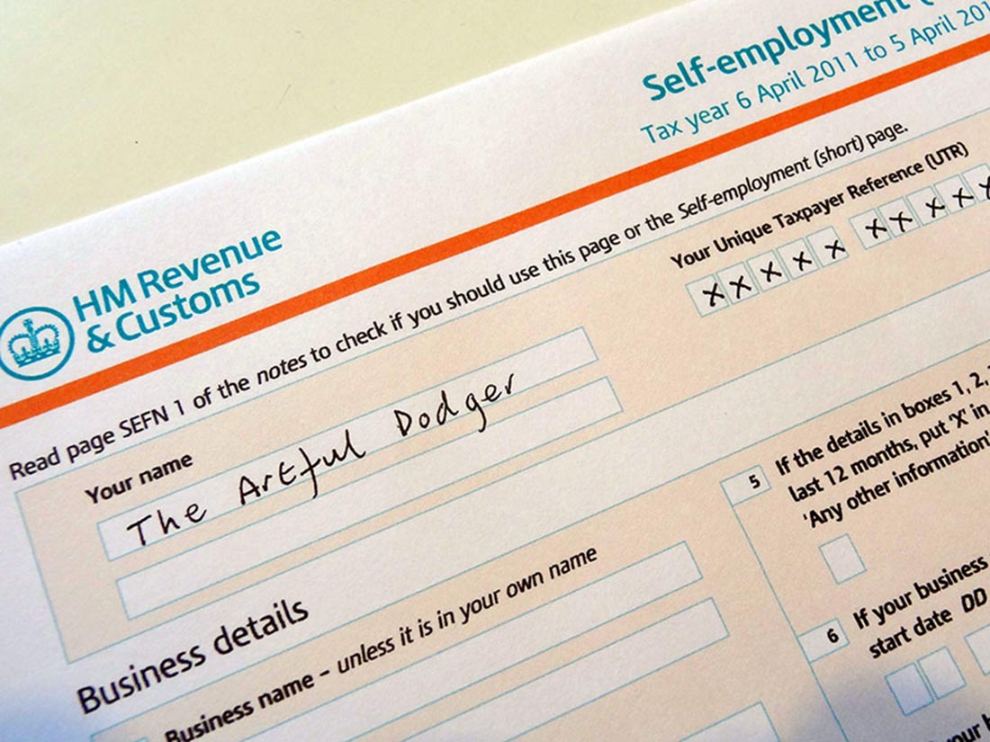
 At an event at the London Palladium on 6 December staged to protest against elements in the recent Budget, the Conservative leader, Kemi Badenoch, was asked whether she would introduce a flat-rate income tax if the Conservatives were returned to government. She replied that it was a very attractive idea. But first the economy would need ‘rewiring’ so that the tax burden could be lightened.
A flat-rate income tax system could take various forms, but the main feature is that there is a single rate of income tax. The specific rate would depend on how much the government wanted to raise. Also it could apply to just income tax, or to both income tax and social insurance (national insurance contributions (NICs) in the UK), or to income tax, social insurance and the withdrawal rate of social benefits. It could also apply to local/state taxes as well as national/federal taxes.
Take the simplest case of a flat-rate income tax with no personal allowance. In this system the marginal and average rate of tax is the same for everyone. This is known as a proportional tax.
Most countries have a progressive income tax system. This normally involves personal allowances (i.e. a zero rate up to a certain level of income) and then various tax bands, with the marginal rate rising when particular tax thresholds are reached. In England, Wales and Northern Ireland, there are three tax bands: 20%, 40% and 45%. Thus the higher a person’s income is, the higher their average rate of tax.
A regressive tax, by contrast, would be one where the average rate of tax fell as incomes rose. The extreme case of a regressive tax would be a lump-sum tax (such as a TV or other licence), which would be same absolute amount for everyone liable to it, irrespective of their income. This was the case with the ‘poll tax’ (or Community Charge, to give it its official title), introduced by Margaret Thatcher’s government in 1989 in Scotland and 1990 in the rest of the UK. It was a local tax, with each taxpayer taxed the same fixed sum, with the precise amount being set by each local authority. After protests and riots, it was replaced in 1993 by the current system of local taxation (Council Tax) based on property values in bands.
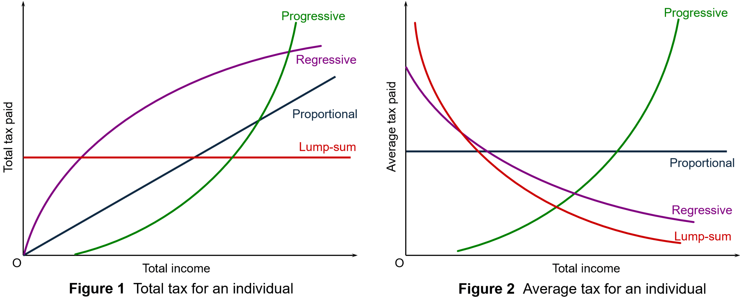
Figures 1 and 2 illustrate these different categories of tax: see Figure 11.12 in Economics, 12th edition. (Click here for a PowerPoint.) Income taxes in most countries are progressive, although just how progressive depends on the differences between the tax bands and the size of personal tax-free allowances. A flat-rate income tax with no allowances is shown by the black line in each diagram, the slope in Figure 1 and the height in Figure 2 depending on the tax rate.
Arguments for a flat-rate income tax
Generally, arguments in favour of flat-rate taxes come from the political right. The two main arguments in favour are tax simplification and incentives.
Advocates argue that a flat tax system makes tax collection easier and makes tax evasion harder. If there are no exemptions, then it can be easier to check that people are paying their taxes and working out the correct amount they owe. It is argued that, in contrast, high tax rates on top earners can encourage tax evasion.
Flat taxes can also be part of a drive to reduce the size of the informal economy. As the VoxEU article states:
Unlike progressive taxes, which include complex and numerous exceptions left to the tax collectors’ discretion, the flat tax is clear cut. In combination with the low rate, its simplicity considerably reduces the stimuli for being informal.
Several post-communist countries in Eastern Europe adopted flat taxes, but for most they were seen as a temporary measure to reduce the informal sector and clamp down on tax evasion. Most have now adopted progressive taxes, with the exceptions of Bulgaria and until recently Russia.
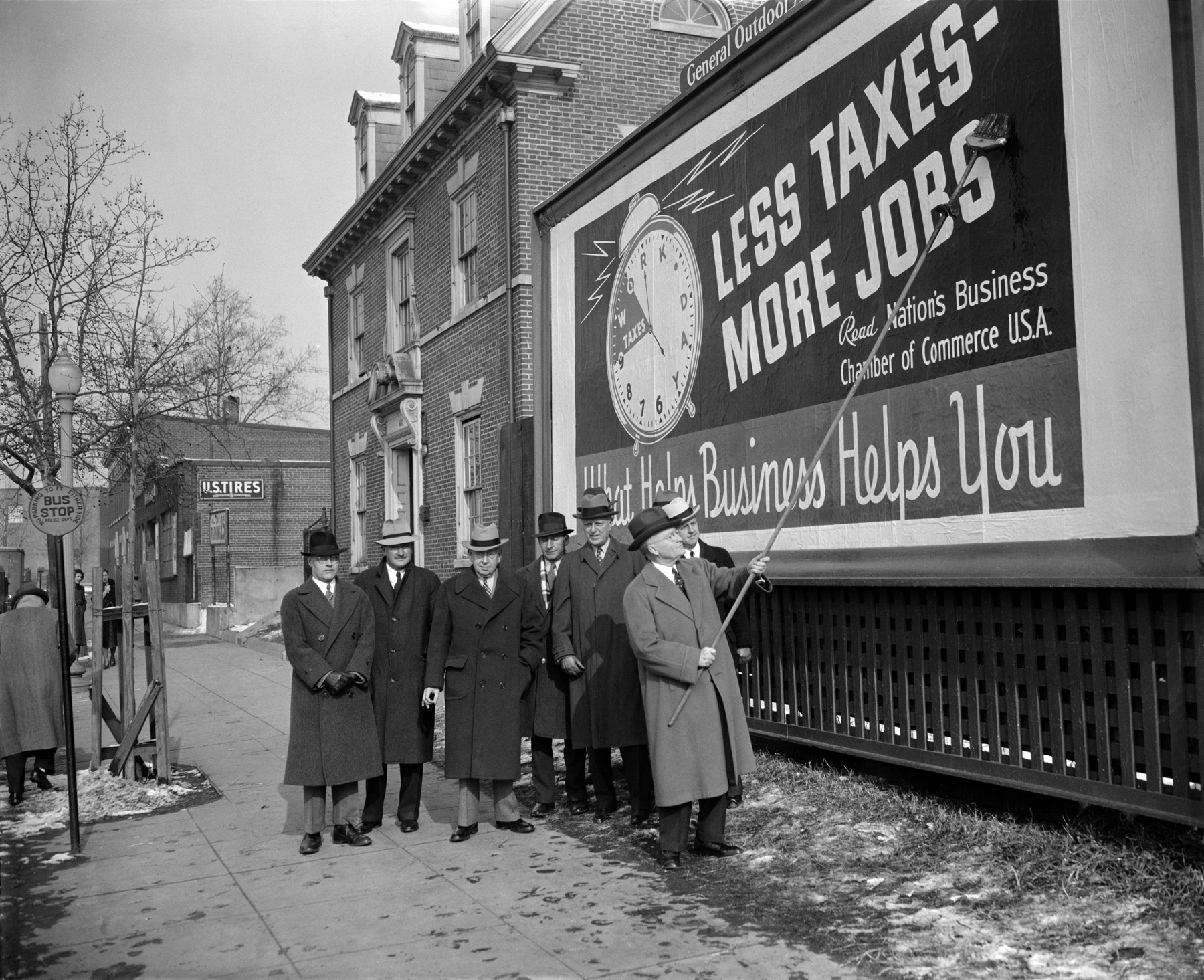 The second major argument is that lower taxes for higher earners, especially for entrepreneurs, can act as a positive incentive. People work harder and there is more investment. The argument here is that the positive substitution effect from the lower tax (work is more profitable now and hence people substitute work for leisure) is greater than the negative income effect (lower taxes increase take-home pay so that people do not need to work so much now to maintain their standard of living).
Then there is the question of tax evasion. With high rates of income tax for top earners, such people may employ accountants to exploit tax loopholes and hide earnings. This could be seen as highly unfair by middle-income earners who are still paying relatively high rates of tax. Even though a move to flat taxes is likely to mean a cut in tax rates for high earners, the tax take from them could be higher. There is evidence that post-communist and developing countries that have adopted flat taxes have found an increase in tax revenues as evasion is harder.
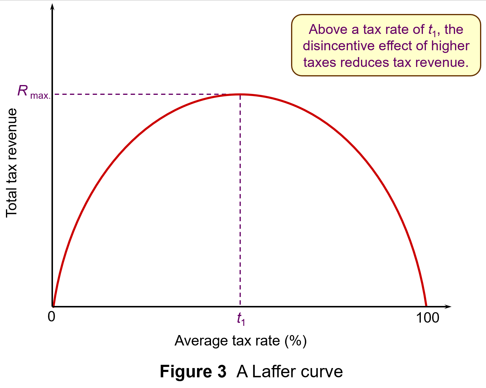 The Laffer curve is often used to illustrate such arguments that high top tax rates can lead to lower tax revenue. Professor Art Laffer was one of President Reagan’s advisers during his first administration (1981–4): see Box 11.3 in Economics, 11th edition. Laffer was a strong advocate of income tax cuts, arguing that substantial increases in output would result and that tax revenues could consequently increase.
The Laffer curve in Figure 3 shows tax revenues increasing as the tax rate increases – but only up to a certain tax rate (t1). Thereafter, tax rates become so high that the resulting fall in output more than offsets the rise in tax rate. When the tax rate reaches 100 per cent, the revenue will once more fall to zero, since no one will bother to work. (Click here for a PowerPoint)
However, as Box 11.3 explains, evidence suggests that tax rates in most countries were well below t1 in the 1980s and certainly are now, given the cuts in income tax rates that have been made around the world over the past 20 years.
Arguments against flat-rate income taxes
 The main argument against moving from a progressive to a flat-rate income tax in an advanced country, such as the UK, is that is would involve a large-scale redistribution of income from the poor to the rich. If the tax were designed to raise the same amount of revenue as at present, those on low incomes would pay more tax than now, as their tax rate would rise to the new flat rate. Those on high incomes would pay less tax, as their marginal rate would fall to the new flat rate.
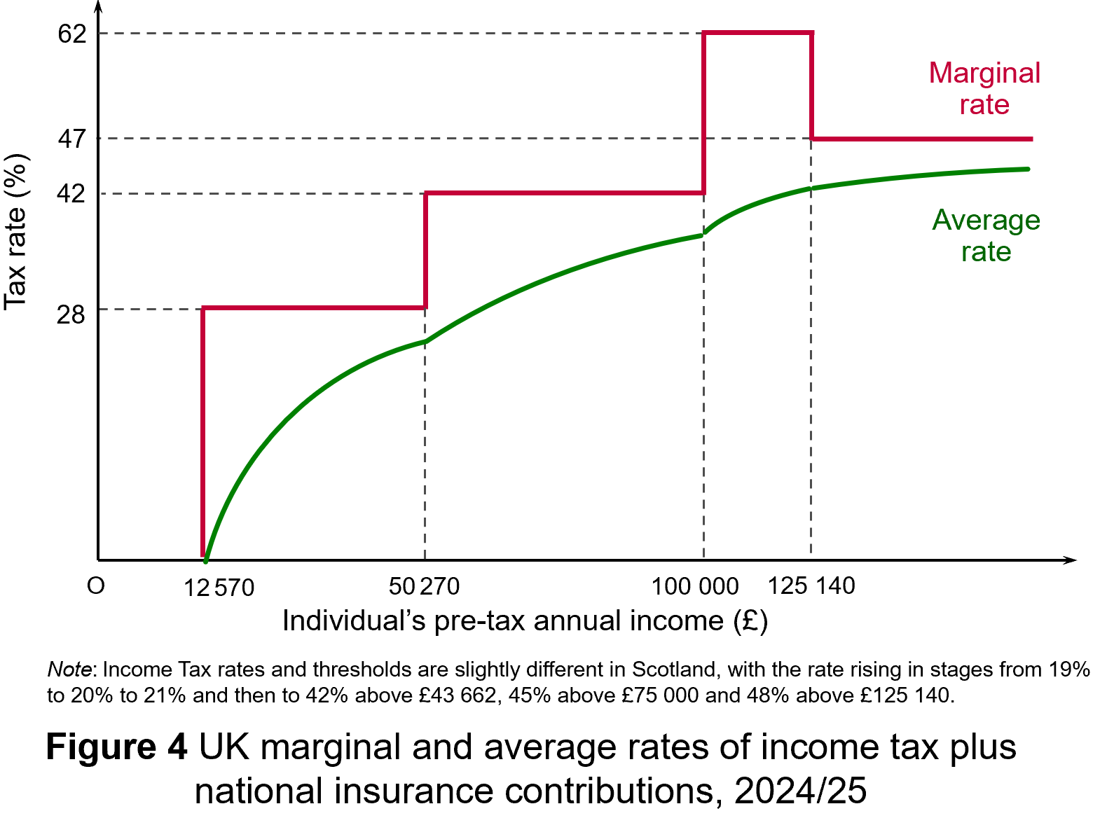
If a new flat-rate tax in the UK also replaced national insurance contributions (NICs), then the effect would be less extreme as NICs are currently initially progressive, as there is a personal allowance before the 8% rate is applied (on incomes above £12 570 in 2024/25). But above a higher NI threshold (£50 270 in 2024/25), the marginal rate drops to 2%, making it a regressive tax beyond that level. Figure 4 shows tax and NI rates in England, Wales and Northern Ireland for 2024/25. (Click here for a PowerPoint.)
 Nevertheless, even if a new flat-rate tax replaced NICs as well as varying rates of income tax, it would still involve a large-scale redistribution from low-income earners to high-income earners. The effect would be mitigated somewhat if personal allowances were raised so that the tax only applied to mid-to-higher incomes. Then the redistribution would be from middle-income earners to high-income earners and also somewhat to low-income earners: i.e. those below, or only a little above, the new higher personal allowance. If, on the other hand, personal allowances were scrapped so that the flat tax applied to all incomes, then there would be a massive redistribution from people on low incomes, including very low incomes, to those on high incomes.
 One of the arguments used to justify a flat-rate tax is that its simplicity would ensure greater compliance. But in an advanced country, compliance is high, except, perhaps, for those on very high incomes. Most people in the UK and many other countries, have tax deducted automatically from their wages. People cannot avoid such taxes.
As far as the self-employed are concerned, they file tax returns online and the software automatically works out the tax due. There are no complex calculations that have to be performed by the individual. There is come scope for tax evasion by charging various expenditures to the business that are really personal spending, but the tax authorities can ask for evidence and sometimes do, with penalties for false claims.
What tax evasion does take place, could still do so with a flat tax. At a rate of, say, 20%, it would still be financially beneficial for a dishonest person to lie if they could get way with it.
Conclusions
If the government did try to introduce a flat-rate income tax, there would probably be an outcry. Also, as some rich people would gain a very large amount of money, the number of people gaining would be lower than the number losing if the total revenue raised were to remain the same. In other words, it would be politically difficult to achieve if the number of losers exceeded the number of gainers.
It is true that if the top rate of income tax were very high, then reducing it might bring in more revenue. But at 45%, or 47% if you include NICs, the top marginal rate in the UK is relatively low compared with other countries. In 2024, the UK had the second lowest top rate of tax out of Western European countries (behind Norway and Switzerland) and only the 16th highest out of 33 European countries when Central and Eastern European countries are also included (see the final ink below under ‘Information’). Reducing the UK’s top rate would be unlikely to bring in more revenue and would redistribute income to high-income earners.
Articles
- Flat tax rate is an ‘attractive idea’, Kemi Badenoch says
The Guardian, Helena Horton (16/12/24)
- Tories could move to a system of ‘flat taxes’ where everyone pays the same rate, Kemi Badenoch indicates
Mail Online, Jason Groves (16/12/24)
- Flat Tax: What It Is and How It Works
Investopedia (8/11/24)
- Flat tax reform in Ukraine: Lessons from Bulgaria
VoxEU, Simeon Djankov (11/12/22)
- Why not… introduce a flat tax?
BBC News, Brian Wheeler (3/7/13)
- Five country cases illustrate how best to improve tax collection
IMF Finance and Development Magazine, Bernardin Akitoby (March 2018)
- Flat taxes and the desire to increase inequality
Funding the Future blog, Richard Murphy (15/5/14)
- Options for a UK ‘flat tax’: some simple simulations
IFS Briefing Note, Stuart Adam and James Browne (August 2006)
- Are the Flat Tax Folks Winning — or Have They Already Won?
Inequality.org, Sam Pizzigati (20/4/24)
Information
Questions
- Distinguish between progressive, proportional, regressive and lump-sum taxes. Into which of these four categories would you place (a) VAT, (b) motor fuel duties, (c) tobacco duties, (d) road-fund licence, (e) inheritance tax? Where the answer is either progressive or regressive, how progressive or regressive are they?
- What are the income and substitution effects of changing tax rates?
- Explain the Laffer curve and consider whether it is likely to be symmetrical.
- Discuss the desirability of having a flat tax set at a relatively high rate (say 25%) with tax-free personal allowances up to the level of income considered to be the poverty threshold. (In the UK the poverty threshold is often defined as 60% of median income.)
- In the London Palladium event where Kemi Badenoch stated that flat taxes were a very attractive idea, she also said that ‘We cannot afford flat taxes where we are now. We need to make sure we rewire our economy so that we can lighten the burden of tax and the regulation on individuals and on those businesses that are just starting out, in particular’. What do you think she meant by this?
- Find out what Bulgaria’s experience of a flat tax of 10% has been.
 In an interview with Joe Rogan for his podcast, The Joe Rogan Experience, just before the US election, Donald Trump stated that, “To me, the most beautiful word – and I’ve said this for the last couple of weeks – in the dictionary today and any is the word ‘tariff’. It’s more beautiful than love; it’s more beautiful than anything. It’s the most beautiful word. This country can become rich with the use, the proper use of tariffs.”
President-elect Trump has stated that he will impose tariffs on imports of 10% or 20%, with 60% and 100% tariffs on imports from China and Mexico, respectively. This protection for US industries, combined with lighter regulation, will, he claims, provide a stimulus to the economy and help create jobs. The revenues will also help to reduce America’s budget deficit.
But it is not that straightforward.
Problems with tariffs for the USA
 Imposing tariffs is likely to reduce international trade. But international trade brings net benefits, which are distributed between the participants according to the terms of trade. This is the law of comparative advantage.
In the simple two-country case, the law states that, provided the opportunity costs of producing various goods differ between the two countries, both of them can gain from mutual trade if they specialise in producing (and exporting) those goods that have relatively low opportunity costs compared with the other country. The total production and consumption of the two countries will be higher.
So if the USA has a comparative advantage in various manufactured products and a trading partner has a comparative advantage in tropical food products, such as coffee or bananas, both can gain by specialisation and trade.
If tariffs are imposed and trade is thereby reduced between the USA and its trading partners, there will be a net loss, as production will switch from lower-cost production to higher-cost production. The higher costs of less efficient production in the USA will lead to higher prices for those goods than if they were imported.
 At the same time, goods that are still imported will be more expensive as the price will include the tariff. Some of this may be borne by the importer, meaning that only part of the tariff is passed on to the consumer. The incidence of the tariff between consumer and importer will depend on price elasticities of demand and supply. Nevertheless, imports will still be more expensive, allowing the domestically-produced substitutes to rise in price too, albeit probably by not so much. According to work by Kimberly Clausing and Mary E Lovely for the Peterson Institute (see link in Articles below), Trump’s proposals to raise tariffs would cost the typical American household over $2600 a year.
The net effect will be a rise in inflation – at least temporarily. Yet one of Donald Trump’s pledges is to reduce inflation. Higher inflation will, in turn, encourage the Fed to raise interest rates, which will dampen investment and economic growth.
Donald Trump tends to behave transactionally rather than ideologically. He is probably hoping that a rapid introduction of tariffs will then give the USA a strong bargaining position with foreign countries to trade more fairly. He is also hoping that protecting US industries by the use of tariffs, especially when coupled with deregulation, will encourage greater investment and thereby faster growth.
Much will depend on how other countries respond. If they respond by raising tariffs on US exports, any gain to industries from protection from imports will be offset by a loss to exporters.
A trade war, with higher tariffs, will lead to a net loss in global GDP. It is a negative sum game. In such a ‘game’, it is possible for one ‘player’ (country) to gain, but the loss to the other players (countries) will be greater than that gain.
 Donald Trump is hoping that by ‘winning’ such a game, the USA could still come out better off. But the gain from higher investment, output and employment in the protected industries would have to outweigh the losses to exporting industries and from higher import prices.
The first Trump administration (2017–21), as part of its ‘America First’ programme, imposed large-scale tariffs on Chinese imports and on steel and aluminium from across the world. There was wide-scale retaliation by other countries with tariffs imposed on a range of US exports. There was a net loss to world income, including US GDP.
Problems with US tariffs for the rest of the world
The imposition of tariffs by the USA will have considerable effects on other countries. The higher the tariffs and the more that countries rely on exports to the USA, the bigger will the effect be. China and Mexico are likely to be the biggest losers as they face the highest tariffs and the USA is a major customer. In 2023, US imports from China were worth $427bn, while US exports to China were worth just $148bn – only 34.6% of the value of imports. The percentage is estimated to be even lower for 2024 at around 32%. In 2023, China’s exports to the USA accounted for 12.6% of its total exports; Mexico’s exports to the USA accounted for 82.7% of its total exports.
It is possible that higher tariffs could be extended beyond China to other Asian countries, such as Vietnam, South Korea, Taiwan, India and Indonesia. These countries typically run trade surpluses with the USA. Also, many of the products from these countries include Chinese components.
As far as the UK is concerned, the proposed tariffs would cause significant falls in trade. According to research by Nicolò Tamberi at the University of Sussex (see link below in Articles):
The UK’s exports to the world could fall by £22 billion (–2.6%) and imports by £1.4 (–0.16%), with significant variations across sectors. Some sectors, like fishing and petroleum, are particularly hard-hit due to their high sensitivity to tariff changes, while others, such as textiles, benefit from trade diversion as the US shifts demand away from China.
Other badly affected sectors would include mining, pharmaceuticals, finance and insurance, and business services. The overall effect, according to the research, would be to reduce UK output by just under 1%.
Countries are likely to respond to US tariffs by imposing their own tariffs on US imports. World Trade Organization rules permit the use of retaliatory tariffs equivalent to those imposed by the USA. The more aggressive the resulting trade war, the bigger would be the fall in world trade and GDP.
The EU is planning to negotiate with Trump to avoid a trade war, but officials are preparing the details of retaliatory measures should the future Trump administration impose the threatened tariffs. The EU response is likely to be strong.
Articles
 The Most Beautiful Word In The Dictionary: Tariffs
YouTube, Joe Rogan and Donald Trump
- The exact thing that helped Trump win could become a big problem for his presidency
CNN, Matt Egan (7/11/24)
- Trump’s New Trade War With China Is Coming
Newsweek, Micah McCartney (9/11/24)
- Trump tariff threat looms large on several Asian countries – not just China – says Goldman Sachs
CNBC, Lee Ying Shan (11/11/24)
- Trump’s bigger tariff proposals would cost the typical American household over $2,600 a year
Peterson Institute for International Economics, Kimberly Clausing and Mary E Lovely (21/8/24)
- More tariffs, less red tape: what Trump will mean for key global industries
The Guardian, Jasper Jolly, Dan Milmo, Jillian Ambrose and Jack Simpson (7/11/24)
- Trump tariffs would halve UK growth and push up prices, says thinktank
The Guardian, Larry Elliott (6/11/24)
- China is trying to fix its economy – Trump could derail those plans
BBC News, João da Silva (8/11/24)
- Trump tariffs could cost UK £22bn of exports
BBC News, Faisal Islam & Tom Espiner (8/11/24)
- Trump to target EU over UK in trade war as he wants to see ‘successful Brexit’, former staffer claims
Independent, Millie Cooke (11/11/24)
- EU’s trade war nightmare gets real as Trump triumphs
Politico, Camille Gijs (6/11/24)
- Will Trump impose his tariffs? They could reduce the UK’s exports by £22 billion.
Centre for Inclusive Trade Policy, University of Sussex, Nicolò Tamberi (8/11/24)
- Three possible futures for the global economy if Trump brings in new trade tariffs
The Conversation, Agelos Delis and Sami Bensassi (17/12/24)
Questions
- Explain why, according to the law of comparative advantage, all countries can gain from trade.
- In what ways may the imposition of tariffs benefit particular sections of an economy?
- Is it in countries’ interests to retaliate if the USA imposes tariffs on their exports to the USA?
- Why is a trade war a ‘negative sum game’?
- Should the UK align with the EU in resisting President-elect Trump’s trade policy or should it seek independently to make a free-trade deal with the USA? is it possible to do both?
- What should China do in response to US threats to impose tariffs of 60% or more on Chinese imports to the USA?
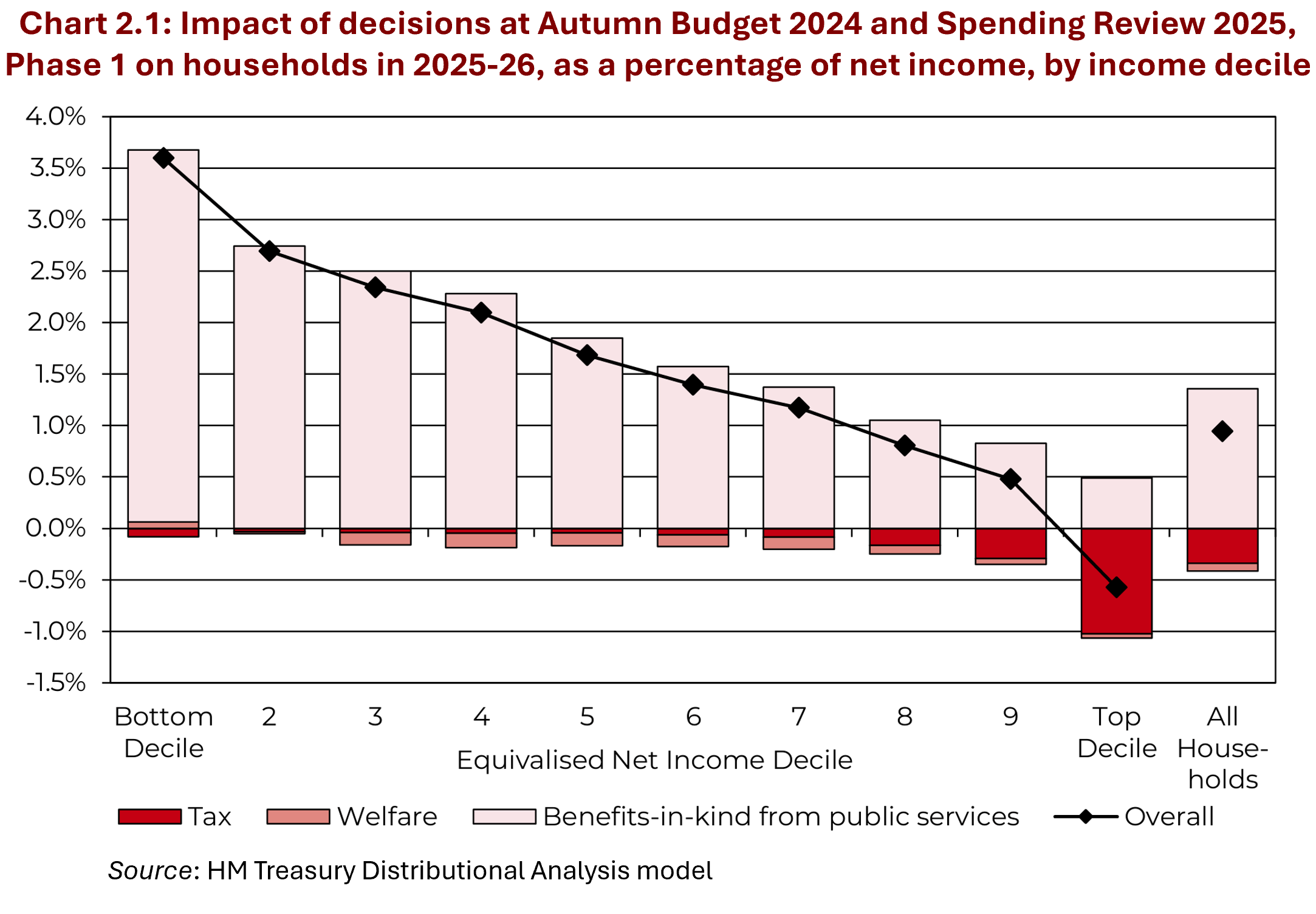 The first Budget of the new UK Labour government was announced on 30 October 2024. It contained a number of measures that will help to tackle inequality. These include extra spending on health and education. This will benefit households on lower incomes the most as a percentage of net income. Increases in tax, by contrast, will be paid predominantly by those on higher incomes. The Chart opposite (taken from the Budget Report) illustrates this. It shows that the poorest 10% will benefit from the largest percentage gain, while the richest 10% will be the only decile that loses.
But one of the major ways of tackling inequality and poverty was raising the minimum wage. The so-called ‘National Living Wage (NLW)’, paid to those aged 21 and over, will rise in April by 6.7% – from £11.44 to £12.41 per hour. The minimum wage paid to those aged 18 to 20 will rise 16.3% from £8.60 to £10.00 and for 16 and 17 year-olds and apprentices it will rise £18% from £6.40 to £7.55.
 It has been an objective of governments for several years to relate the minimum wage to the median wage. In 2015, the Conservative Government set a target of raising the minimum wage rate to 60 per cent of median hourly earnings by 2020. When that target was hit a new one was set to reach two-thirds of median hourly earnings by 2024.
The Labour government has set a new remit for the minimum wage (NLW). There are two floors. The first is the previously agreed one, that the NLW should be at least two-thirds of median hourly earnings; the second is that it should fully compensate for cost of living rises and for expected inflation up to March 2026. The new rate of £12.41 will meet both criteria. According to the Low Pay Commission, ‘Wages have risen faster than inflation over the past 12 months, and are forecast to continue to do so up to March 2026’. This makes the first floor the dominant one: meeting the first floor automatically meets the second.
How effective is the minimum wage in reducing poverty and inequality?
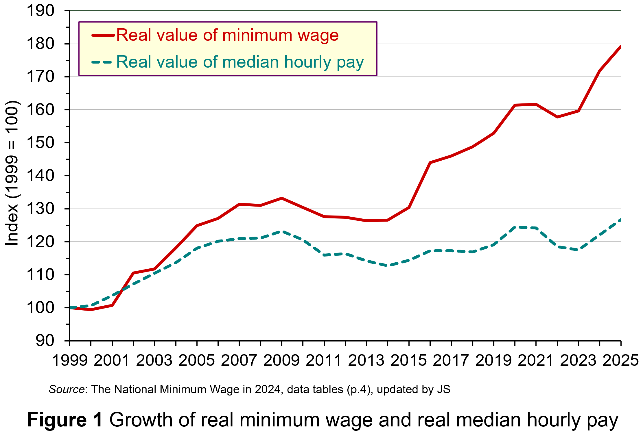 Figure 1 shows the growth in minimum wage rates since their introduction in 1999. The figures are real figures (i.e. after taking into account CPI inflation) and are expressed as an index, with 1999 = 100. The chart also shows the growth in real median hourly pay. (Click here for a Powerpoint.)
As you can see, the growth in real minimum wage rates has considerably exceeded the growth in real median hourly pay. This has had a substantial effect on raising the incomes of the poorest workers and thereby has helped to reduce poverty and inequality.
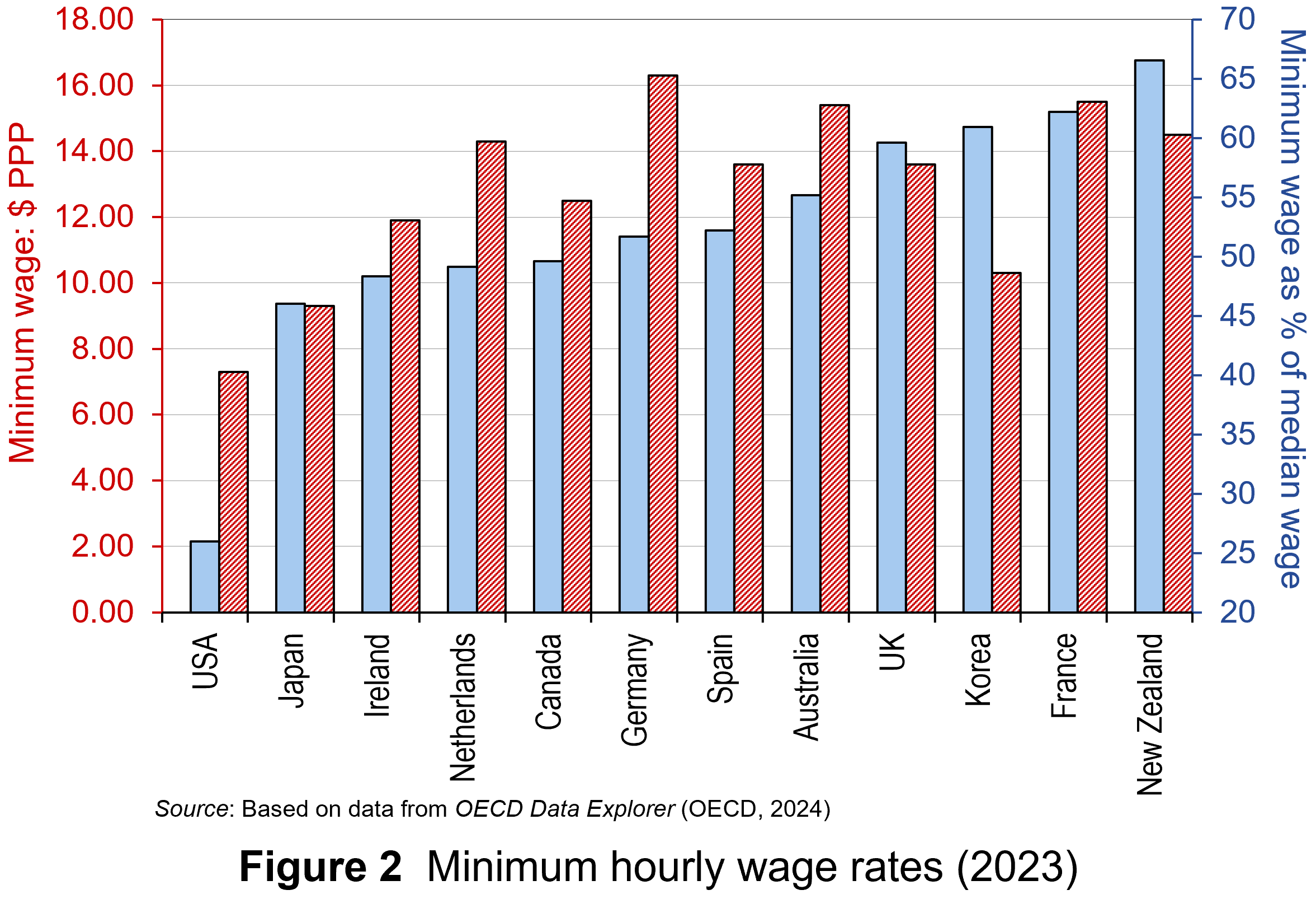 The UK minimum wage compares relatively favourably with other high-income economies. Figure 2 shows minimum wage rates in 12 high-income countries in 2023 – the latest year for which data are available. (Click here for a PowerPoint.) The red bars (striped) show hourly minimum wage rates in US dollars at purchasing-power parity (PPP) rates. PPP rates correct current exchange rates to reflect the purchasing power of each country’s currency. The blue bars (plain) show minimum wage rates as a percentage of the median wage rate. In 2023 the UK had the fourth highest minimum wage of the 12 countries on this measure (59.6%). As we have seen above, the 2025 rate is expected to be 2/3 of the median rate.
Minimum wages are just one mechanism for reducing poverty and inequality. Others include the use of the tax and benefit system to redistribute incomes. The direct provision of services, such as health, education and housing at affordable rents can make a significant difference and, as we have seen, have been a major focus of the October 2024 Budget.
The government has been criticised, however, for not removing the two-child limit to extra benefits in Universal Credit (introduced in 2017). The cap clearly disadvantages poor families with more than two children. What is more, for workers on Universal Credit, more than half of the gains from the higher minimum wages will lost because they will result in lower benefit entitlement. Also the freeze in (nominal) personal income tax allowances will mean more poor people will pay tax even with no rise in real incomes.
Effects on employment: analysis
A worry about raising the minimum wage rate is that it could reduce employment in firms already paying the minimum wage and thus facing a wage rise.
In the case of a firm operating in competitive labour and goods markets, the demand for low-skilled workers is relatively wage sensitive. Any rise in wage rates, and hence prices, by this firm alone would lead to a large fall in sales and hence in employment.
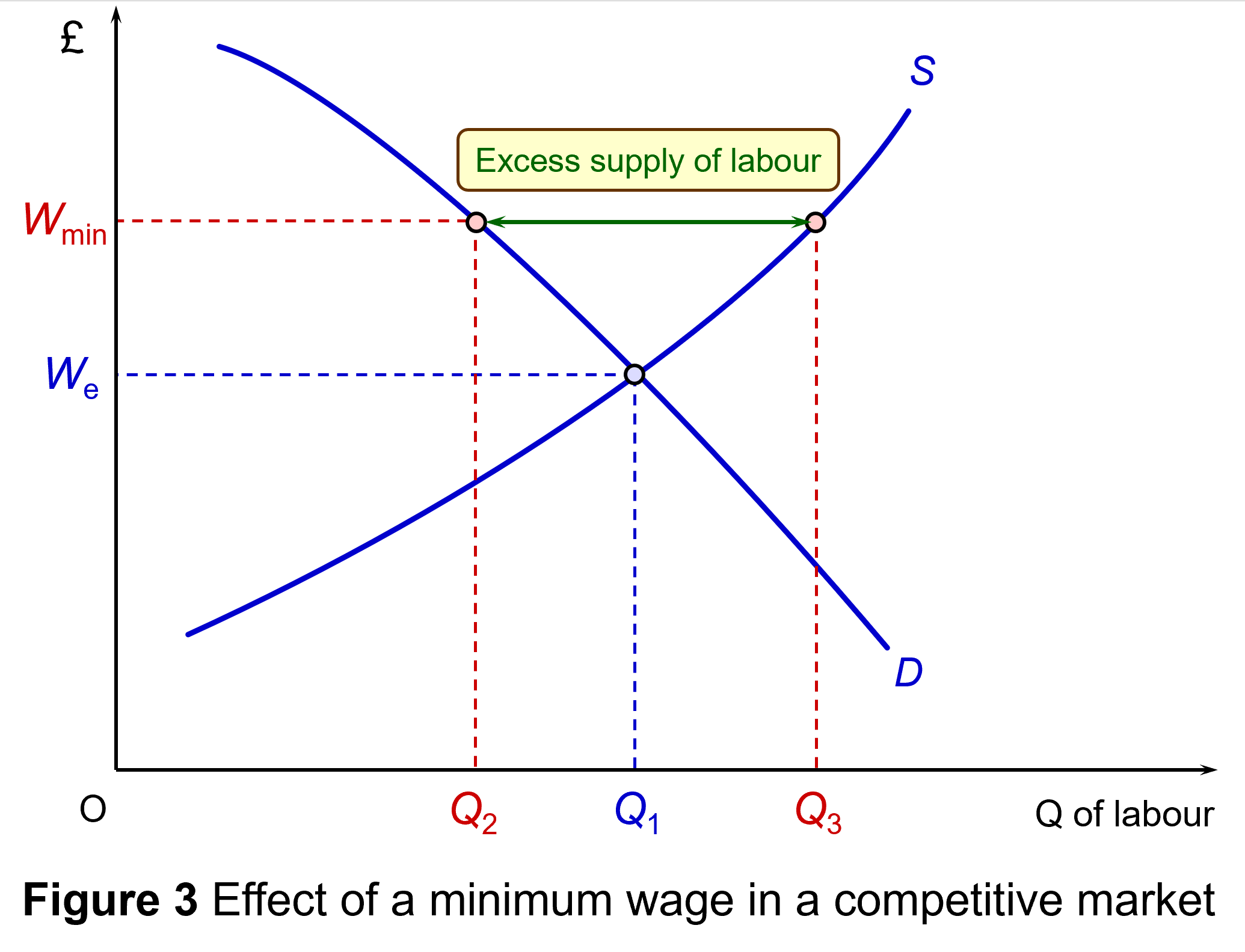 This is illustrated in Figure 3 (click here for a PowerPoint). Assume that the minimum wage is initially the equilibrium wage rate We. Now assume that the minimum wage is raised to Wmin. This will cause a surplus of labour (i.e. unemployment) of Q3 – Q2. Labour supply rises from Q1 to Q3 and the demand for labour falls from Q1 to Q2.
But, given that all firms face the minimum wage, individual employers are more able to pass on higher wages in higher prices, knowing that their competitors are doing the same. The quantity of labour demanded in any given market will not fall so much – the demand is less wage elastic; and the quantity of labour supplied in any given market will rise less – the supply is less wage elastic. Any unemployment will be less than that illustrated in Figure 3. If, at the same time, the economy expands so that the demand-for-labour curve shifts to the right, there may be no unemployment at all.
When employers have a degree of monopsony power, it is not even certain that they would want to reduce employment. This is illustrated in Figure 4: click here for a PowerPoint (you can skip this section if you are not familiar with the analysis).
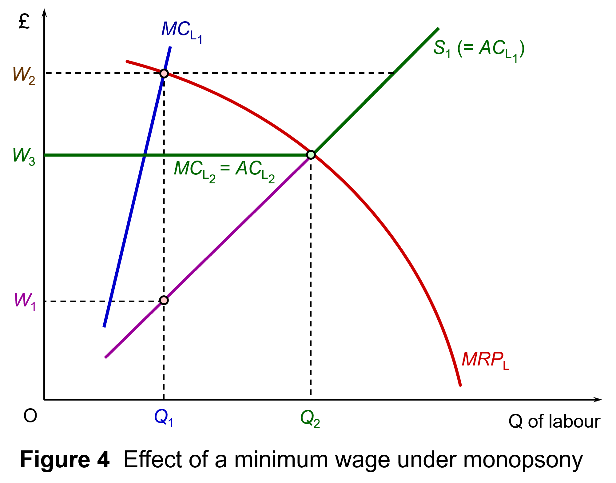 Assume initially that there is no minimum wage. The supply of labour to the monopsony employer is given by curve SL1, which is also the average cost of labour ACL1. A higher employment by the firm will drive up the wage; a lower employment will drive it down. This gives a marginal cost of labour curve of MCL1. Profit-maximising employment will be Q1, where the marginal cost of labour equals the marginal revenue product of labour (MRPL). The wage, given by the SL1 (=ACL1) line will be W1.
Now assume that there is a minimum wage. Assume also that the initial minimum wage is at or below W1. The profit-maximising employment is thus Q1 at a wage rate of W1.
The minimum wage can be be raised as high as W2 and the firm will still want to employ as many workers as at W1. The point is that the firm can no longer drive down the wage rate by employing fewer workers, and so the ACL1 curve becomes horizontal at the new minimum wage and hence will be the same as the MCL curve (MCL2 = ACL2). Profit-maximising employment will be where the MRPL curve equals this horizontal MCL curve. The incentive to cut its workforce, therefore, has been removed.
Again, if we extend the analysis to the whole economy, a rise in the minimum wage will be partly passed on in higher prices or stimulate employers to increase labour productivity. The effect will be to shift the (MRPL) curve upwards to the right, thereby allowing the firm to pass on higher wages and reducing any incentive to reduce employment.
Effects on employment: evidence
There is little evidence that raising the minimum wage in stages will create unemployment, although it may cause some redeployment. In the Low Pay Commission’s 2019 report, 20 years of the National Minimum Wage (see link below), it stated that since 2000 it had commissioned more than 30 research projects looking at the NMW’s effects on hours and employment and had found no strong evidence of negative effects. Employers had adjusted to minimum wages in various ways. These included reducing profits, increasing prices and restructuring their business and workforce.
Along with our commissioned work, other economists have examined the employment effects of the NMW in the UK and have for the most part found no impact. This is consistent with international evidence suggesting that carefully set minimum wages do not have noticeable employment effects. While some jobs may be lost following a minimum wage increase, increasing employment elsewhere offsets this. (p.20)
There is general agreement, however, that a very large increase in minimum wages will impact on employment. This, however, should not be relevant to the rise in the NLW from £11.44 to £12.41 per hour in April 2025, which represents a real rise of around 4.5%. This at worst should have only a modest effect on employment and could be offset by economic growth.
 What, however, has concerned commentators more is the rise in employers’ National Insurance contributions (NICs) that were announced in the Budget. In April 2025, the rate will increase from 13.8% to 15%. Employers’ NICs are paid for each employee on all wages above a certain annual threshold. This threshold will fall in April from £9100 to £5000. So the cost to an employer of an employee earning £38 000 per annum in 2024/25 would be £38 000 + ((£38 000 – £9100) × 0.138) = £41 988.20. For the year 2025/26 it will rise to £38 000 + ((£38 000 – £5000) × 0.15) = £42 950. This is a rise of 2.29%. (Note that £38 000 will be approximately the median wage in 2025/26.)
However, for employees on the new minimum wage, the percentage rise in employer NICs will be somewhat higher. A person on the new NLW of £12.41, working 40 hours per week and 52 weeks per year (assuming paid holidays), will earn an annual wage of £25 812.80. Under the old employer NIC rates, the employer would have paid (£25 812.80 + (£25 812.80 – £9100) × 0.138) = £28 119.17. For the year 2025/26, it will rise to £25 812.80 + ((£25 812.80 – £5000) × 0.15) = £28 934.72. This is a rise of 2.90%.
This larger percentage rise in employers’ wage costs for people on minimum wages than those on median wages, when combined with the rise in the NLW, could have an impact on the employment of those on minimum wages. Whether it does or not will depend on how rapid growth is and how much employers can absorb the extra costs through greater productivity and/or passing on the costs to their customers.
Articles
- National Living Wage to increase to £12.21 in April 2025
Low Pay Commission, Press Release (29/10/24)
- Rachel Reeves hands low-paid a £1,400 boost as minimum wage to rise by 6.7%
Independent, Archie Mitchell and Millie Cooke (31/10/24)
- Minimum wage to rise to £12.21 an hour next year
BBC News, Michael Race (29/10/24)
- What Labour’s first budget means for wages, taxes, business, the NHS and plans to grow the economy – experts explain
The Conversation, Rachel Scarfe et al. (30/10/24)
- The two-child limit: poverty, incentives and cost
Institute for Fiscal Studies, Eduin Latimer and Tom Waters (17/6/24)
UK Government reports and information
Data
Questions
- How is the October 2024 Budget likely to affect the distribution of income?
- What are the benefits and limitations of statutory minimum wages in reducing (a) poverty and (b) inequality?
- Under what circumstances will a rise in the minimum wage lead or not lead to an increase in unemployment?
- Find out what is meant by the UK Real Living Wage (RLW) and distinguish it from the UK National Living Wage (NLW). Why is the RLW higher?
- Why is the median wage rather than the mean wage used in setting the NLW?
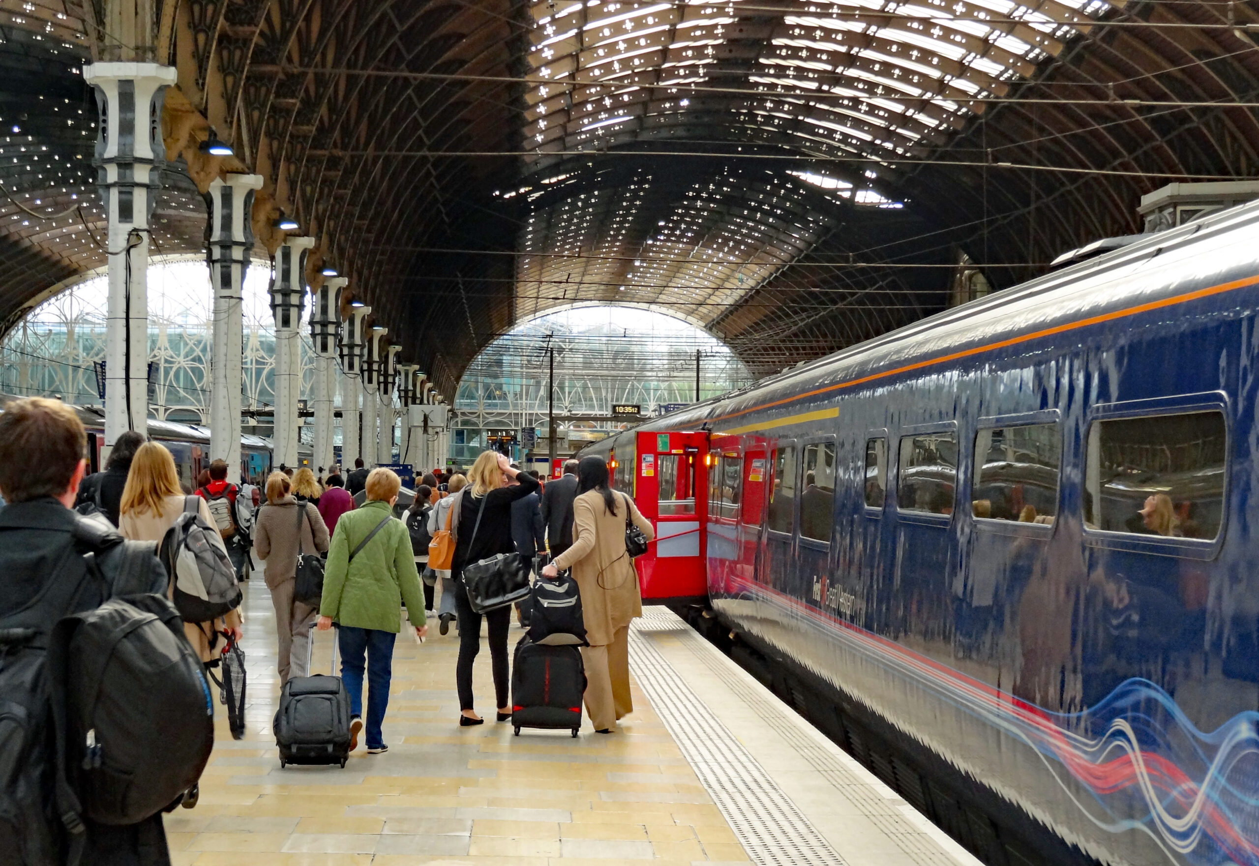 In many countries, train fares at peak times are higher than at off-peak times. This is an example of third-degree price discrimination. Assuming that peak-time travellers generally have a lower price elasticity of demand, the policy allows train companies to increase revenue and profit.
If the sole purpose of ticket sales were to maximise profits, the policy would make sense. Assuming that higher peak-time fares were carefully set, although the number travelling would be somewhat reduced, this would be more than compensated for by the higher revenue per passenger.
But there are external benefits from train travel. Compared with travel by car, there are lower carbon emissions per person travelling. Also, train travel helps to reduce road congestion. To the extent that higher peak-time fares encourage people to travel by car instead, there will be resulting environmental and congestion externalities.
The Scottish experiment with abolishing higher peak-time fares
 In October 2023, the Scottish government introduced a pilot scheme abolishing peak-time fares, so that tickets were the same price at any time of the day. The idea was to encourage people, especially commuters, to adopt more sustainable means of transport. Although the price elasticity of demand for commuting is very low, the hope was that the cross-price elasticity between cars and trains would be sufficiently high to encourage many people to switch from driving to taking the train.
One concern with scrapping peak-time fares is that trains would not have the capacity to cope with the extra passengers. Indeed, one of the arguments for higher peak-time fares is to smooth out the flow of passengers during the day, encouraging those with flexibility of when to travel to use the cheaper and less crowded off-peak trains.
This may well apply to certain parts of the UK, but in the case of Scotland it was felt that there would be the capacity to cope with the extra demand at peak time. Also, in a post-COVID world, with more people working flexibly, there was less need for many people to travel at peak times than previously.
Reinstatement of peak-time fares in Scotland
It was with some dismay, therefore, especially by commuters and environmentalists, when the Scottish government decided to end the pilot at the beginning of October 2024 and reinstate peak-time fares – in many cases at nearly double the off-peak rates. For example, the return fare between Glasgow and Edinburgh rose from £16.20 to £31.40 at peak times.
The Scottish government justified the decision by claiming that passenger numbers had risen by only 6.8%, when, to be self-financing, an increase of 10% would have been required. But this begs the question of whether it was necessary to be self-financing when the justification was partly environmental. Also, the 6.8% figure is based on a number of assumptions that could be challenged (see The Conversation article linked below). A longer pilot would have helped to clarify demand.
Other schemes
A number of countries have introduced schemes to encourage greater use of the railways or other forms of public transport. One of these is the flat fare for local journeys. Provided that this is lower than previously, it can encourage people to use public transport and leave their car at home. Also, its simplicity is also likely to be attractive to passengers. For example, in England bus fares are capped at £2. Currently, the scheme is set to run until 31 December 2024.
 Another scheme is the subscription model, whereby people pay a flat fee per month (or week or year, or other time period) for train or bus travel or both. Germany, for example, has a flat-rate €49 per month ‘Deutschland-Ticket‘ (rising to €58 per month in January 2025). This ticket provides unlimited access to local and regional public transport in Germany, including trains, buses, trams, metros and ferries (but not long-distance trains). This zero marginal fare cost of a journey encourages passengers to use public transport. The only marginal costs they will face will be ancillary costs, such as getting to and from the train station or bus stop and having to travel at a specific time.
Articles
- Why a pilot scheme removing peak rail fares should have been allowed to go the distance
The Conversation, Rachel Scarfe (8/10/24)
- Return of peak rail fares a costly blow for commuters and climate, Scottish Greens say
Bright Green, Chris Jarvis (6/10/24)
 Commuters react to return of peak train fares in Scotland
BBC News (1/10/24)
- Perth peak rail fares to Edinburgh rise by almost 60 percent as pilot scheme ends
Daily Record, Alastair McNeill (4/10/24)
- Ditch peak-time rail fares across UK, campaigners say
iNews, Adam Forrest (30/9/24)
- Train fares reduced by up to 20% in East Yorkshire
Rail Advent, Roger Smith (26/9/24)
- Deutschland-Ticket: Germany’s popular monthly transport pass will soon be more expensive
Euronews, Angela Symons (24/9/24)
- Fare Britannia: a new approach to public transport ticketing for the UK
Greenpeace report, Leo Eyles, Tony Duckenfield and Jim Steer (19/9/24)
- Ministers urged to trial monthly ‘climate card’ in North of England to save rail commuters money and cut emissions
About Manchester, Nigel Barlow (20/9/24)
Questions
- Identify the arguments for and against having higher rail fares at peak times than at off-peak times
- Why might it be a good idea to scrap higher peak-time fares in some parts of a country but not in others?
- Provide a critique of the Scottish government’s arguments for reintroducing higher peak-time fares.
- With reference to The Conversation article, why is it difficult to determine the effect on demand of the Scottish pilot of scrapping peak-time fares?
- What are the arguments for and against the German scheme of having a €49 per month public transport pass for local and regional transport with no further cost per journey? Should it be extended to long-distance trains and coaches?
- In England there is a flat £2 single fare for buses. Would it be a good idea to make bus travel completely free?
 On Saturday 31 August, tickets for the much-heralded Oasis reunion tour went on sale through the official retailer, Ticketmaster. When the company sells tickets, the acts or their promoters can choose whether to use a static pricing system, where each type of ticket is sold at a set price until they have all been sold. Or they can use a dynamic pricing system (‘in-demand’ or ‘platinum’ tickets, as Ticketmaster calls them), where there is a starting price quoted, but where prices then rise according to demand. The higher the demand, the more the price is driven up. Acts or their promoters have the option of choosing an upper limit to the price.
Dynamic pricing
The Oasis tickets were sold under the dynamic pricing system, a system previously used for Harry Styles, Bruce Springsteen, Coldplay and Blackpink concerts, but one rejected by Taylor Swift for her recent Eras tour. Standing tickets for the Oasis concert with a face value of around £135 were quickly being sold for over £350. There were long online queues, with the prices rising as people slowly moved up the queue. When they reached the front, they had to decide quickly whether to pay the much higher price. Some people later suffered from buyer’s remorse, when they realised that in the pressure of the moment, they had paid more than they could afford.
Dynamic pricing is when prices change with market conditions: rising at times when demand exceeds supply and falling when supply exceeds demand. It is sometimes referred to as ‘surge pricing’ to reflect situations when price surges in times of excess demand.
Dynamic pricing is a form of price discrimination. It is an imperfect form of first-degree price discrimination, which is defined as people being charged the maximum price they are willing to pay for a product. Pricing in an eBay auction comes close to first-degree price discrimination. With dynamic pricing in the ticket market, some people may indeed pay the maximum, but others earlier in the queue will be lucky and pay less than their maximum.
Ticketmaster justifies the system of dynamic pricing, saying that it gives ‘fans fair and safe access to the tickets, while enabling artists and other people involved in staging live events to price tickets closer to their true market value’. The company argues that if the price is below the market value, a secondary market will then drive ticket prices up. Ticket touts will purchase large amounts of tickets, often using bots to access the official site and then resell them at highly inflated prices on sites such as Viagogo and Stubhub, where ticket prices for popular acts can sell for well over £1000. The day after Oasis tickets went on sale, Viagogo had seats priced at up to £26 000 each!
Oasis and Ticketmaster have tried to stamp out the unofficial secondary market by stating that only tickets bought through the official retailers (Ticketmaster, Gigsandtours and SeeTickets) will be valid. If fans want to resell a ticket – perhaps because they find they can no longer go – they can resell them on the official secondary market though Ticketmaster’s Fan-to-Fan site or Twickets. These official secondary sites allow holders of unwanted tickets to sell them for anything up to the original face value, but no more. Buyers pay a 12% handling fee. It remains to be seen whether this can be enforced with genuine tickets resold on the secondary market.
Examples of dynamic pricing
 Dynamic pricing is not a new pricing strategy. It has been used for many years in the transport, e-commerce and hospitality sectors. Airlines, for example, have a pricing model whereby as a flight fills up, so the prices of the seats rise. If you book a seat on a budget airline a long time in advance, you may be able to get it at a very low price. If, on the other hand, you want a seat at the last minute, you may well have to pay a very high price. The price reflects the strength of demand and its price elasticity. The business traveller who needs to travel the next day for a meeting will have a very low price sensitivity and may well be prepared to pay a very high price indeed. Airlines also learn from past behaviour and so some popular routes will start at a higher price. A similar system of dynamic pricing is used with advance train tickets, with the price rising as trains get booked up.
The dynamic pricing system used by airlines and train companies is similar, but not identical, to first-degree price discrimination. The figure below illustrates first-degree price discrimination by showing a company setting the price for a particular product.
Assume initially that it sets a single profit-maximising price. This would be a price of P1, at an output of Q1, where marginal revenue (MR) equals marginal cost (MC). (We assume for simplicity that average and marginal costs are constant.) Total profit will be area 1: i.e. the blue area ((P1 – AC) × Q1). Area 2 represents consumer surplus, with all those consumers who would have been prepared to pay a price above P1, only having to pay P1.
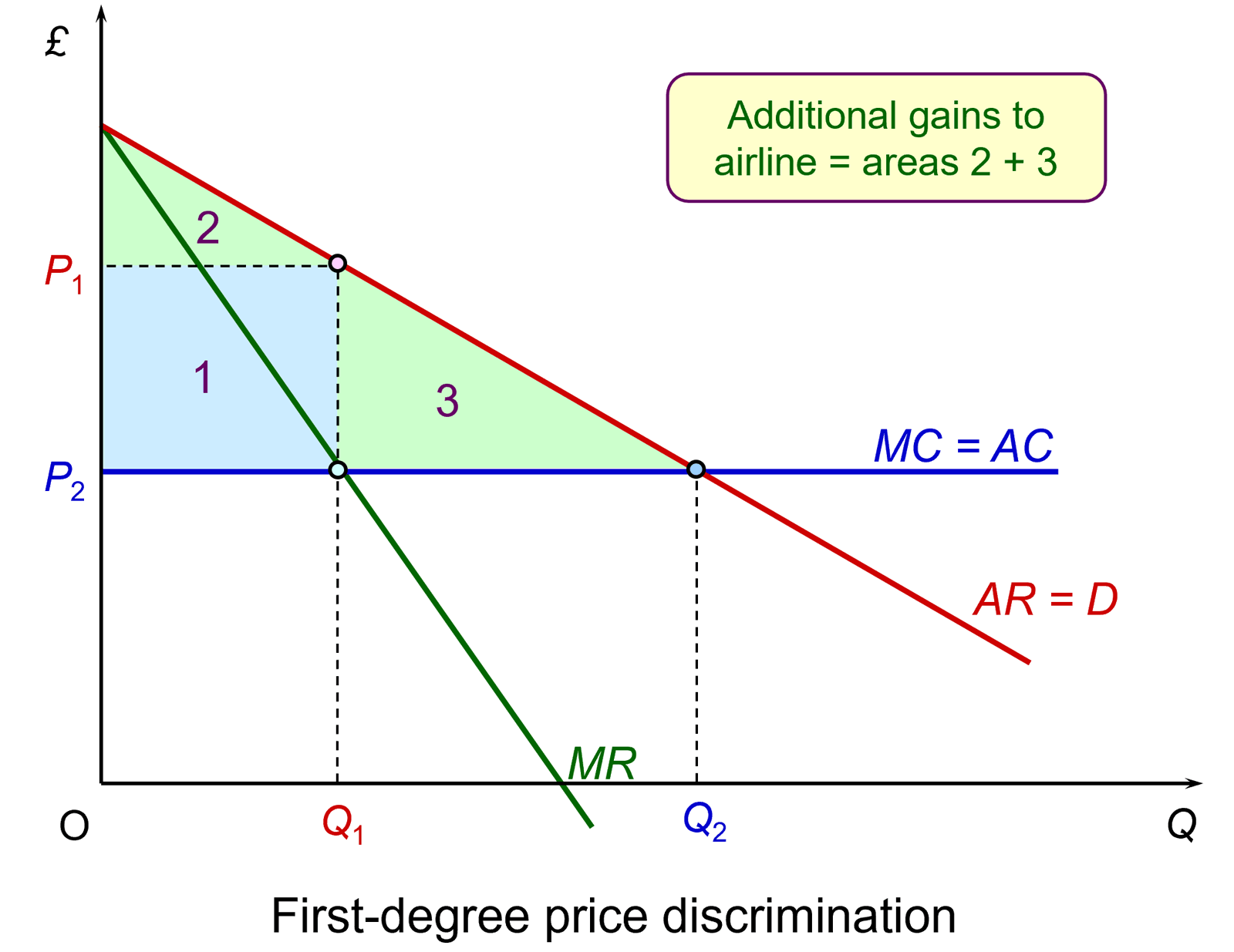 Now assume that the firm uses first-degree price discrimination, selling each unit of the product at the maximum price each consumer is willing to pay. Starting with the consumer only willing to pay a price of P2, the price will go on rising up along the demand with each additional consumer being charged a higher price up to the price where the demand curve meets the vertical axis. In such a case, the firm’s profit would be not just the blue area, but also the green areas 2 and 3. Note that there is no consumer surplus as area 2 is now part of the additional profit to the firm.
Although dynamic pricing by airlines is similar to this model of first-degree price discrimination, in practice some people will be paying less than they would be willing to pay and the price goes up in stages, not continuously with each new sale of a ticket. Thus, compared with a fixed price per seat, the additional profit will be less than areas 2 + 3, but total profit will still be considerably greater than area 1 alone. Note also that there is a maximum quantity of seats (Qmax), represented by a full flight. The airline would hope that demand and its pricing model are such that Qmax is less than Q2.
Dynamic pricing also applies in the hospitality sector, as hotels raise the prices for rooms according to demand, with prices at peak times often being considerably higher than off-season prices. Rather then pre-setting prices for particular seasons, dates or weekends/weekdays, many hotels, especially chains and booking agents, adjust prices dynamically as demand changes. Airbnb offers property owners what it calls ‘Smart Pricing’, where nightly prices change automatically with demand.
 Another example is Uber, which uses dynamic pricing to balance demand and supply location by location. In times of peak demand on any route, the company’s algorithm will raise the price. This will encourage people to delay travelling if they can or use alternative means of transport. It will also encourage more Uber drivers to come to that area. In times of low demand, the price will fall. This will encourage more people to use the service (rather than regular taxis or buses) and discourage drivers from working in that area.
Where dynamic pricing varies with the time or date when the purchase is made, it is sometimes referred to as inter-temporal pricing. It is a form of second-degree price discrimination, which is where a firm offers consumers a range of different pricing options for the same or similar products.
Another example of dynamic pricing, which is closer to first-degree price discrimination is the use of sophisticated algorithms and AI by Amazon, allowing it to update the prices of millions of products many times a day according to market conditions. Another is eBay auctions, where the price rises as the end date is reached, according to the willingness to pay of the bidders.
Attitudes to dynamic pricing
Consumers have grown accustomed to dynamic pricing in many industries. People generally accept the pricing model of budget airlines, for example. What makes it acceptable is that most people feel that they can take advantage of early low-priced seats and can compare the current prices on different flights and airlines when making their travel plans. Pricing is transparent. With the Oasis concert, however, there wasn’t the same degree of price transparency. Many people were surprised and dismayed to find that when they got to the front of the online queue, the price had risen dramatically.
People are familiar of dynamic pricing in the context of price cuts to shift unsold stock. Supermarkets putting stickers on products saying ‘reduced for quick sale’ is an example. Another is seasonal sales. What is less acceptable to many consumers is firms putting up prices when demand is high. They see it a profiteering. Many supermarkets are introducing electronic shelf labels (ESLs), where prices can be changed remotely as demand changes. Consumers may react badly to this if they see the prices going up. The supermarket, however, may find it a very convenient way of reducing prices to shift stock – something consumers are hardly likely to complain about.
 Returning to the Oasis tour, the UK government responded to the outrage of fans as ticket prices soared. Culture Secretary, Lisa Nandy, announced that the government will investigate how surge pricing for concert tickets is used by official retailers, such as Ticketmaster. This will be part of a planned review of ticket sales that seeks to establish a fairer and more transparent system of pricing.
The problem is that, with some fans being prepared to pay very high prices indeed to see particular acts and with demand considerably exceeding supply at prices that fans would consider reasonable, some way needs to be found of rationing demand. If it is not price, then it will inevitably involve some form of queuing or rationing system, with the danger that this encourages touts and vastly inflated prices on the secondary market.
Perhaps a lesson can be drawn from the Glastonbury Festival, where prices are fixed, people queue online and where security systems are in place to prevent secondary sales by ticket touts. The 2024 price was set at £355 + a £5 booking fee and purchasers were required to register with personal details and a photo, which was checked on admission.
Update
On 5 September, the CMA announced that it was launching an investigation into Ticketmaster over the Oasis concert sales. Its concerns centred on ‘whether buyers were given clear and timely information, and whether consumer protection law was breached’. This followed complaints by fans that (i) they were not given clear and timely information beforehand that the tickets involved dynamic pricing and warned about the possible prices they might have to pay and (ii) on reaching the front of the queue they were put under pressure to buy tickets within a short period of time.
Meanwhile, band member stated that they were unaware that dynamic pricing would be used and that the decision to use the system was made by their management.
Videos
Articles
- Oasis ticket sales – everything you need to know about reunion
BBC News (27/8/24)
- Ticketmaster demand-based pricing system criticised
BBC News, Annabel Rackham (10/10/22)
- I loved Oasis – until I saw Ticketmaster’s dynamic pricing
Metro, Issy Packer (2/9/24)
- A supersonic swindle: my £1,423 Oasis Ticketmaster hell
The Guardian, Josh Halliday (1/9/24)
- Bands urged to oppose dynamic pricing of concert tickets after Oasis ‘fiasco’
The Guardian, Josh Halliday and Rob Davies (1/9/24)
- Oasis tickets: what is dynamic pricing and why is it used for live music?
The Guardian, Rob Davies (1/9/24)
- Viagogo defends reselling Oasis tickets for thousands of pounds as ‘legal’
City A.M. (31/8/24)
- Oasis fans face ‘eye-watering’ resale ticket prices
i News, Adam Sherwin (30/8/240
- Would you really pay €500 for an Oasis ticket?
RTE Brainstorm, Emma Howard (3/9/24)
- When ‘dynamic pricing’ works – and when it doesn’t
Investors’ Chronicle, Hermione Taylor (11/12/23)
- The pros, cons and misconceptions of dynamic pricing for retailers
Computer Weekly, Glynn Davis (20/6/24)
- Dynamic Pricing (Taylor’s Version)
Linkedin, Economic Insight (10/7/23)
- Dynamic pricing: successful companies that use this pricing strategy
PriceTweakers, Simon Gomez (25/5/24)
- Five lessons for businesses investigating dynamic pricing
FT Strategies
- Inflated Oasis ticket prices ‘depressing’ – government promises review of dynamic pricing
Sky News (2/9/24)
- Lisa Nandy hits out at ‘incredibly depressing’ Oasis ticket sale and orders probe into surge pricing
Independent, Archie Mitchell (2/9/24)
- Oasis ticket row: How Ticketmaster’s owner has grip on UK live music scene
BBC News, Chi Chi Izundu and James Stewart (4/9/24)
- CMA launches investigation into Ticketmaster over Oasis concert sales
CMA Press Release (5/9/24)
- Revealed: the touts offering Oasis tickets for thousands on resale sites
The Guardian, Rob Davies, Hannah Al-Othman and Tiago Rogero (7/9/24)
Questions
- What is the difference between dynamic pricing and surge pricing?
- What is buyer’s remorse? How could dynamic pricing be used while minimising the likelihood of buyer’s remorse?
- Distinguish between first-degree, second-degree and third-degree price discrimination. Do the various forms of dynamic pricing correspond to one or more of these three types?
- Distinguish between consumer and producer surplus. How may dynamic pricing lead to a reduction in consumer surplus and an increase in producer surplus?
- Should Ticketmaster sell tickets on the same basis as tickets for the Glastonbury Festival?
- Is Oasis a monopoly? What are the ticket pricing implications?
- Are there any industries where firms would not benefit from dynamic pricing? Explain.
- What are the arguments for and against allowing tickets to be sold on the secondary market for whatever price they will fetch?
- How powerful is Ticketmaster in the primary and secondary ticket markets?
 At an event at the London Palladium on 6 December staged to protest against elements in the recent Budget, the Conservative leader, Kemi Badenoch, was asked whether she would introduce a flat-rate income tax if the Conservatives were returned to government. She replied that it was a very attractive idea. But first the economy would need ‘rewiring’ so that the tax burden could be lightened.
 The second major argument is that lower taxes for higher earners, especially for entrepreneurs, can act as a positive incentive. People work harder and there is more investment. The argument here is that the positive substitution effect from the lower tax (work is more profitable now and hence people substitute work for leisure) is greater than the negative income effect (lower taxes increase take-home pay so that people do not need to work so much now to maintain their standard of living).
 The Laffer curve is often used to illustrate such arguments that high top tax rates can lead to lower tax revenue. Professor Art Laffer was one of President Reagan’s advisers during his first administration (1981–4): see Box 11.3 in Economics, 11th edition. Laffer was a strong advocate of income tax cuts, arguing that substantial increases in output would result and that tax revenues could consequently increase.
  The main argument against moving from a progressive to a flat-rate income tax in an advanced country, such as the UK, is that is would involve a large-scale redistribution of income from the poor to the rich. If the tax were designed to raise the same amount of revenue as at present, those on low incomes would pay more tax than now, as their tax rate would rise to the new flat rate. Those on high incomes would pay less tax, as their marginal rate would fall to the new flat rate.
 Nevertheless, even if a new flat-rate tax replaced NICs as well as varying rates of income tax, it would still involve a large-scale redistribution from low-income earners to high-income earners. The effect would be mitigated somewhat if personal allowances were raised so that the tax only applied to mid-to-higher incomes. Then the redistribution would be from middle-income earners to high-income earners and also somewhat to low-income earners: i.e. those below, or only a little above, the new higher personal allowance. If, on the other hand, personal allowances were scrapped so that the flat tax applied to all incomes, then there would be a massive redistribution from people on low incomes, including very low incomes, to those on high incomes.
 One of the arguments used to justify a flat-rate tax is that its simplicity would ensure greater compliance. But in an advanced country, compliance is high, except, perhaps, for those on very high incomes. Most people in the UK and many other countries, have tax deducted automatically from their wages. People cannot avoid such taxes.
 In an interview with Joe Rogan for his podcast, The Joe Rogan Experience, just before the US election, Donald Trump stated that, “To me, the most beautiful word – and I’ve said this for the last couple of weeks – in the dictionary today and any is the word ‘tariff’. It’s more beautiful than love; it’s more beautiful than anything. It’s the most beautiful word. This country can become rich with the use, the proper use of tariffs.”
 Imposing tariffs is likely to reduce international trade. But international trade brings net benefits, which are distributed between the participants according to the terms of trade. This is the law of comparative advantage.
 At the same time, goods that are still imported will be more expensive as the price will include the tariff. Some of this may be borne by the importer, meaning that only part of the tariff is passed on to the consumer. The incidence of the tariff between consumer and importer will depend on price elasticities of demand and supply. Nevertheless, imports will still be more expensive, allowing the domestically-produced substitutes to rise in price too, albeit probably by not so much. According to work by Kimberly Clausing and Mary E Lovely for the Peterson Institute (see link in Articles below), Trump’s proposals to raise tariffs would cost the typical American household over $2600 a year.
 Donald Trump is hoping that by ‘winning’ such a game, the USA could still come out better off. But the gain from higher investment, output and employment in the protected industries would have to outweigh the losses to exporting industries and from higher import prices.
 The first Budget of the new UK Labour government was announced on 30 October 2024. It contained a number of measures that will help to tackle inequality. These include extra spending on health and education. This will benefit households on lower incomes the most as a percentage of net income. Increases in tax, by contrast, will be paid predominantly by those on higher incomes. The Chart opposite (taken from the
  It has been an objective of governments for several years to relate the minimum wage to the median wage. In 2015, the Conservative Government set a target of raising the minimum wage rate to 60 per cent of median hourly earnings by 2020. When that target was hit a new one was set to reach two-thirds of median hourly earnings by 2024.
 Figure 1 shows the growth in minimum wage rates since their introduction in 1999. The figures are real figures (i.e. after taking into account CPI inflation) and are expressed as an index, with 1999 = 100. The chart also shows the growth in real median hourly pay. (Click
  The UK minimum wage compares relatively favourably with other high-income economies. Figure 2 shows minimum wage rates in 12 high-income countries in 2023 – the latest year for which data are available. (Click
  This is illustrated in Figure 3 (click
  Assume initially that there is no minimum wage. The supply of labour to the monopsony employer is given by curve SL1, which is also the average cost of labour ACL1. A higher employment by the firm will drive up the wage; a lower employment will drive it down. This gives a marginal cost of labour curve of MCL1. Profit-maximising employment will be Q1, where the marginal cost of labour equals the marginal revenue product of labour (MRPL). The wage, given by the SL1 (=ACL1) line will be W1.
  What, however, has concerned commentators more is the rise in employers’ National Insurance contributions (NICs) that were announced in the Budget. In April 2025, the rate will increase from 13.8% to 15%. Employers’ NICs are paid for each employee on all wages above a certain annual threshold. This threshold will fall in April from £9100 to £5000. So the cost to an employer of an employee earning £38 000 per annum in 2024/25 would be £38 000 + ((£38 000 – £9100) × 0.138) = £41 988.20. For the year 2025/26 it will rise to £38 000 + ((£38 000 – £5000) × 0.15) = £42 950. This is a rise of 2.29%. (Note that £38 000 will be approximately the median wage in 2025/26.)
 In many countries, train fares at peak times are higher than at off-peak times. This is an example of third-degree price discrimination. Assuming that peak-time travellers generally have a lower price elasticity of demand, the policy allows train companies to increase revenue and profit.
  In October 2023, the Scottish government introduced a pilot scheme abolishing peak-time fares, so that tickets were the same price at any time of the day. The idea was to encourage people, especially commuters, to adopt more sustainable means of transport. Although the price elasticity of demand for commuting is very low, the hope was that the cross-price elasticity between cars and trains would be sufficiently high to encourage many people to switch from driving to taking the train.
 Another scheme is the subscription model, whereby people pay a flat fee per month (or week or year, or other time period) for train or bus travel or both. Germany, for example, has a flat-rate €49 per month ‘
 On Saturday 31 August, tickets for the much-heralded Oasis reunion tour went on sale through the official retailer, Ticketmaster. When the company sells tickets, the acts or their promoters can choose whether to use a static pricing system, where each type of ticket is sold at a set price until they have all been sold. Or they can use a dynamic pricing system (‘in-demand’ or ‘platinum’ tickets, as Ticketmaster calls them), where there is a starting price quoted, but where prices then rise according to demand. The higher the demand, the more the price is driven up. Acts or their promoters have the option of choosing an upper limit to the price.
 Dynamic pricing is not a new pricing strategy. It has been used for many years in the transport, e-commerce and hospitality sectors. Airlines, for example, have a pricing model whereby as a flight fills up, so the prices of the seats rise. If you book a seat on a budget airline a long time in advance, you may be able to get it at a very low price. If, on the other hand, you want a seat at the last minute, you may well have to pay a very high price. The price reflects the strength of demand and its price elasticity. The business traveller who needs to travel the next day for a meeting will have a very low price sensitivity and may well be prepared to pay a very high price indeed. Airlines also learn from past behaviour and so some popular routes will start at a higher price. A similar system of dynamic pricing is used with advance train tickets, with the price rising as trains get booked up.
 Now assume that the firm uses first-degree price discrimination, selling each unit of the product at the maximum price each consumer is willing to pay. Starting with the consumer only willing to pay a price of P2, the price will go on rising up along the demand with each additional consumer being charged a higher price up to the price where the demand curve meets the vertical axis. In such a case, the firm’s profit would be not just the blue area, but also the green areas 2 and 3. Note that there is no consumer surplus as area 2 is now part of the additional profit to the firm.
 Another example is Uber, which uses dynamic pricing to balance demand and supply location by location. In times of peak demand on any route, the company’s algorithm will raise the price. This will encourage people to delay travelling if they can or use alternative means of transport. It will also encourage more Uber drivers to come to that area. In times of low demand, the price will fall. This will encourage more people to use the service (rather than regular taxis or buses) and discourage drivers from working in that area.
 Returning to the Oasis tour, the UK government responded to the outrage of fans as ticket prices soared. Culture Secretary, Lisa Nandy, announced that the government will investigate how surge pricing for concert tickets is used by official retailers, such as Ticketmaster. This will be part of a planned review of ticket sales that seeks to establish a fairer and more transparent system of pricing.