 This is the second of three blogs looking at high inflation and its implications. Here we look at changes in the housing market and its effects on households. Another way of analysing the financial importance of the housing and mortgage markets is through the balance sheets and associated flow accounts of the household sector.
We used the concept of balance sheets in our blog Bank failures and the importance of balance sheets. In the blog we referred to the balance-sheet effects from interest rate hikes on the financial well-being of financial institutions.
The analysis is analogous for households. Again, we can identify two general effects: rising borrowing and debt-servicing costs, and easing asset prices.
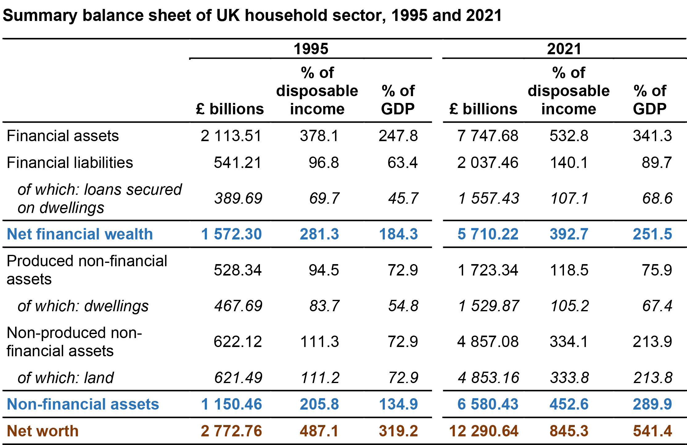
The following table shows the summary balance sheet of the UK household sector in 1995 and 2021.
Source: National balance sheet estimates for the UK: 1995 to 2021 (January 2023) and series RPHA, ONS
The total value of the sector’s net wealth (or ‘worth’) is the sum of its net financial wealth and its non-financial assets. The former is affected by the value of the stock of outstanding mortgages, which we can see from row 3 in the table (‘loans secured on dwellings’) has increased from £390 billion in 1995 to £1.56 trillion in 2021. This is equivalent to an increase from 70 to 107 per cent of the sector’s annual disposable income. This increase helps to understand the sensitivity of the sector’s financial position to interest rate increases and the sizeable cash flow effects. These effects then have implications for the sector’s spending.
 Housing is also an important asset on household balance sheets. The price of housing reflects both the value of dwellings and the land on which they sit, and these are recorded separately on the balance sheets. Their combined balance sheet value increased from £1.09 trillion (£467.69bn + £621.49bn) in 1995 to £6.38 trillion (£1529.87bn + £4853.16bn) in 2021 or from 128% of GDP to 281%.
The era of low inflation and low interest rates that had characterised the previous two decades or so had helped to boost house price growth and thus the value of non-financial assets on the balance sheets. In turn, this had helped to boost net worth, which increased from £2.78 trillion in 1995 to £12.29 trillion in 2021 or from 319% of GDP to 541%.
Higher interest rates and wealth
 The advent of higher interest rates was expected not only to impact on the debt servicing costs of households but the value of assets, including, in the context of this blog, housing. As Chart 3 in the previous blog helped to show, higher interest rates and higher mortgage repayments contributed to an easing of house price growth as housing demand eased. On the other hand, the impact on mortgaged landlords helped fuel the growth of rental prices as they passed on their increased mortgage repayment costs to tenants.
Higher interest rates not only affect the value of housing but financial assets such as corporate and government bonds whose prices are inversely related to interest rates. Research published by the Resolution Foundation in July 2023 estimates that these effects are likely to have contributed to a fall in the household wealth from early 2021 to early 2023 by as much as £2.1 trillion.
The important point here is that further downward pressure on asset prices is expected as they adjust to higher interest rates. This and the impact of higher debt servicing costs will therefore continue to impact adversely on general financial well-being with negative implications for the wider macroeconomic environment.
Articles
- The Mortgage Crunch
Resolution Foundation, Simon Pittaway (17/6/23)
- Peaked Interest?
Resolution Foundation, Molly Broome, Ian Mulheirn and Simon Pittaway (17/7/23)
- UK inflation to fall to lowest level since March 2022 but Bank of England still tipped to hike interest rates
City A.M., Jack Barnett (17/7/23)
- Mortgage payments set to jump by £500 for one million households
BBC News, Tom Espiner (13/7/23)
- Interest rates: Big rise less likely after inflation surprise
BBC News, Daniel Thomas, Faisal Islam & Dharshini David (19/7/23)
- Rising Mortgage Costs. What Can Be Done?
NIESR blog, Max Mosley and Adrian Pabst (17/7/23)
- UK interest rates forecast to rise less sharply after inflation falls to 7.9%
The Guardian, Richard Partington (19/7/23)
- Mortgage costs: More Scots falling behind on repayments
Herald Scotland, Kristy Dorsey (18/7/23)
Report
Data
Questions
- What possible indicators could be used to assess the affordability of residential house prices?
- What do you understand by the concept of the monetary policy transmission mechanism? How do the housing and mortgage markets relate to this concept?
- What factors might affect the proportion of people taking out fixed-rate mortgages rather than variable-rate mortgages?
- What is captured by the concept of net worth? Discuss how the housing and mortgage markets affect the household sector’s net worth.
- What are cash-flow effects? How do rising interest rates effect savers and borrowers?
- How might wealth effects from rising interest rates impact younger and older people differently?
- Discuss the ways by which house price changes could affect household consumption.
 This is the first of three blogs looking at inflation, at its effect on household budgets and at monetary policy to bring inflation back to the target rate. This first one takes an overview.
The housing and mortgage markets are vitally important to the financial well-being of many households. We have seen this vividly in recent times through the impact of rising inflation rates on interest rates and, in turn, on mortgage repayments. Some people on variable rate mortgages, or whose fixed rate deals are coming to the end of their term, have struggled to pay the new higher rates. In this blog we explore the reasons behind these events and the extent to which the financial well-being of UK households has been affected.
Chart 1 shows the path of inflation in the UK since 1997 when the Bank of England’s Monetary Policy Committee (MPC) was first charged with meeting an inflation rate target (click here for a PowerPoint). It captures the impact of the inflation shock that began to emerge in 2021 and saw the CPI inflation rate peak at 11.1 per cent in October 2022 – considerably above the Bank’s 2 per cent target.
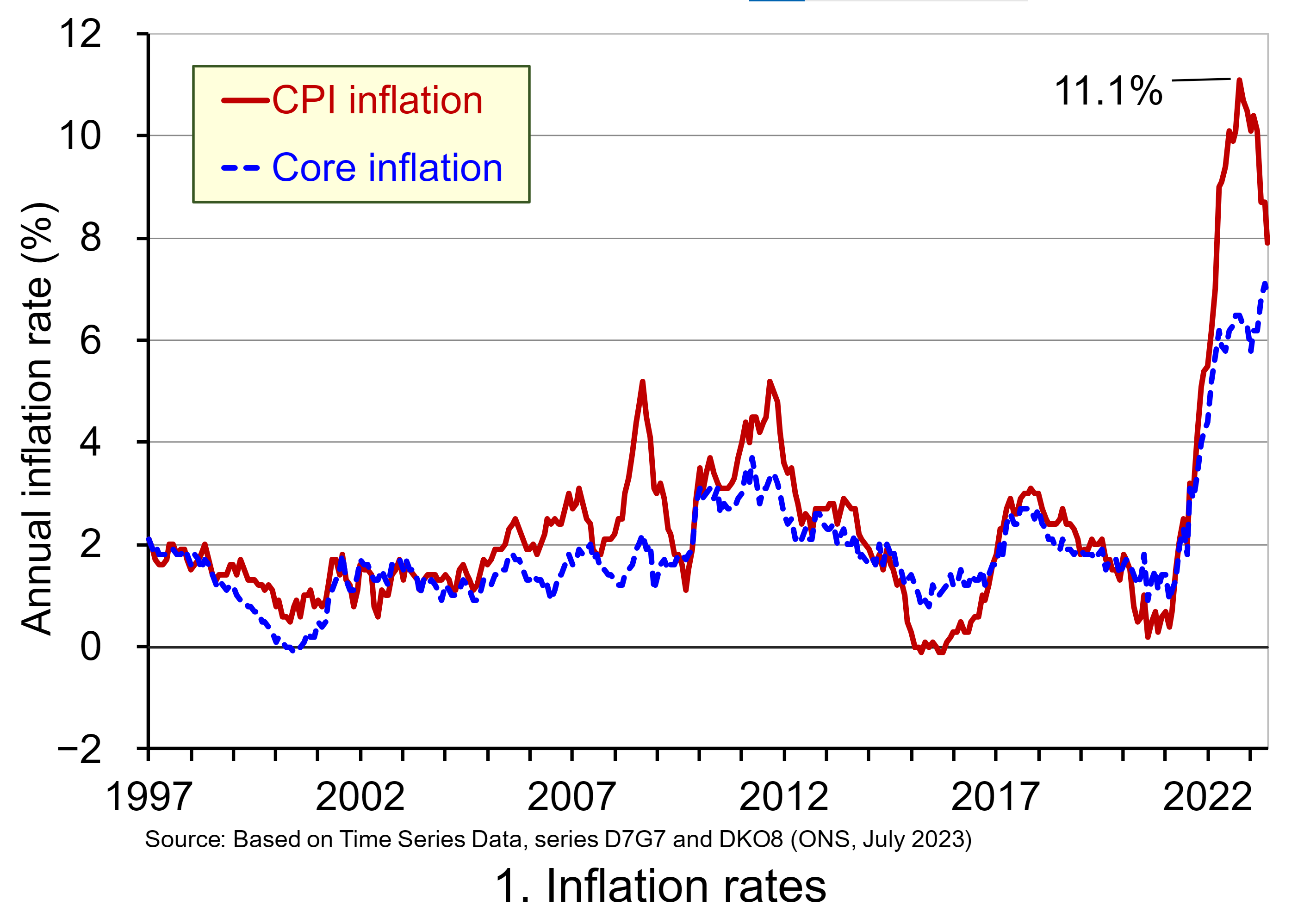 Despite easing somewhat, the CPI inflation rate is showing signs of persistence – meaning that it is taking time for it to return to target. One way of understanding this persistence is to look at a measure of inflation known as core inflation. This inflation rate measure excludes energy, food, alcoholic beverages and tobacco prices, all of which are notoriously volatile. Core inflation thus captures underlying inflationary pressures.
To address the inflationary pressures, the Bank of England began raising Bank Rate in December 2021 from a low of just 0.1 per cent. By June 2023 the Bank Rate had risen to 5 per cent with the prospect of further hikes. As the Bank Rate rises, the cost of borrowing from the Bank of England by commercial banks rises too. Therefore increases in the Bank Rate ripple through to other interest rates. However, the passthrough effect can be uneven affecting spreads between Bank Rate and other interest rates.
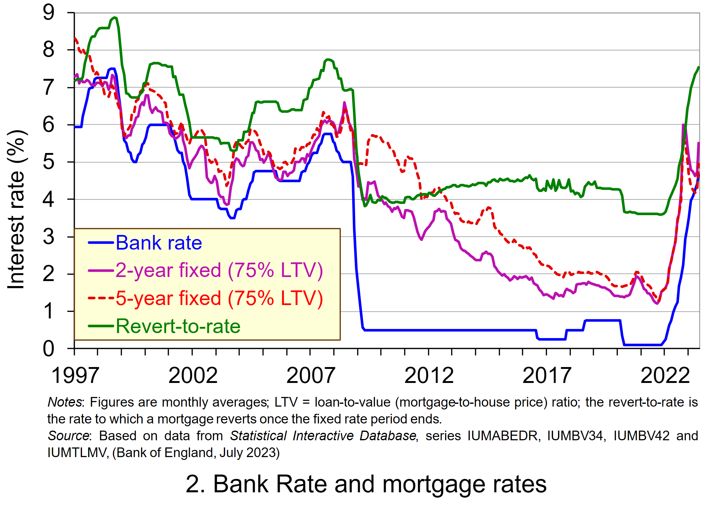 The increase in the Bank Rate is reflected in the increases in mortgage rates shown in Chart 2 (click here for a PowerPoint). As we have seen, this affects most immediately those with variable rate mortgages, and then those with fixed-rate mortgages as they come up for renewal. Analysis from the Resolution Foundation (2023) estimates that 4.2 million households saw their mortgage rates change between December 2021 and June 2023 – the equivalent of 56 per cent of mortgaged households.
The persistence of inflation means that mortgage rates may not have yet peaked and are likely to stay higher for longer than originally thought. With fixes normally between two to five years, the problem of higher rates for those renewing will continue. The Resolution Foundation projects that by the end of 2026, almost all households with a mortgage would have moved to a higher rate since December 2021. At this point, the typical annual repayment cost for mortgaged households is forecast to be £2000 per annum higher, leading to an increase in annual repayments for the UK household sector of £15.8 billion.
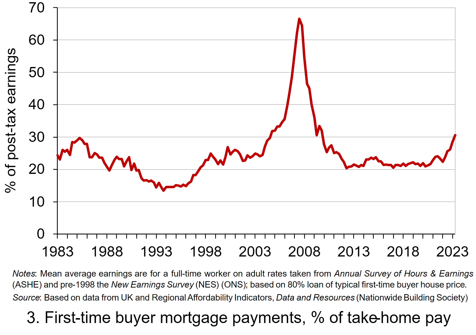 Chart 3 provides a visual picture of the typical annual repayment costs facing first-time buyers as a percentage of earnings after tax and national insurance (click here for a PowerPoint). The Nationwide Building Society figures are based on an 80% loan on the typical first-time buyer house price. It shows that repayment costs have been rising sharply on the back of rising interest rates and are now higher than at any time since the global financial crisis of 2007–8.
Articles
- UK inflation to fall to lowest level since March 2022 but Bank of England still tipped to hike interest rates
City A.M., Jack Barnett (17/7/23)
- UK inflation and interest rates high – how do other economies compare?
BBC News, Dharshini David (23/7/23)
- Mortgage payments set to jump by £500 for one million households
BBC News, Tom Espiner (13/7/23)
- Interest rates: Big rise less likely after inflation surprise
BBC News, Daniel Thomas, Faisal Islam & Dharshini David (19/7/23)
- Rising Mortgage Costs. What Can Be Done?
NIESR blog, Max Mosley and Adrian Pabst (17/7/23)
- UK interest rates forecast to rise less sharply after inflation falls to 7.9%
The Guardian, Richard Partington (19/7/23)
- Mortgage costs: More Scots falling behind on repayments
Herald Scotland, Kristy Dorsey (18/7/23)
- The Mortgage Crunch
Resolution Foundation, Simon Pittaway (17/6/23)
- Peaked Interest?
Resolution Foundation, Molly Broome, Ian Mulheirn and Simon Pittaway (17/7/23)
Data
Questions
- What possible indicators could be used to assess the affordability of residential house prices?
- What is captured by the rate of core inflation? Discuss the arguments for using this as the target inflation rate measure.
- What factors might affect the proportion of people taking out fixed-rate mortgages rather than variable-rate mortgages?
- Discuss the ways by which house price changes could impact on household consumption.
- Investigate the proportion of mortgages that are fixed rate and the typical length of the fixed rate term in two European countries, the USA and Japan. How does each differ from the UK?
 March 2023 saw the failure of Silicon Valley Bank (SVB), a regional US bank based in California that focused on financial services for the technology sector. It also saw the forced purchase of global-banking giant, Credit Suisse, by rival Swiss bank, UBS. These events fuelled concerns over the banking sector’s financial well-being, with fears for other financial institutions and the wider economy.
Yet it is not the only sector where concerns abound over financial well-being. The cost-of-living crisis, the hike in interest rates and the economic slowdown continue to have an adverse impact on the finances of households and businesses. Furthermore, many governments face difficult fiscal choices in light of the effects of recent economic shocks, such as COVID and the Russian invasion of Ukraine, on the public finances.
Balance sheets and flow accounts
When thinking about the financial well-being of people, business and governments it is now commonplace for economists to reference balance sheets. This may seem strange to some since it is easy to think of balance sheets as the domain of accountants or those working in finance. Yet balance sheets, and the various accounts that lie behind them, are essential in analysing financial well-being and, therefore, in helping to understand economic behaviour and outcomes. Hence, it is important for economists to embrace them too.
 A balance sheet is a record of stocks of assets and liabilities of individuals or organisations. Behind these stocks are accounts capturing flows, including income, expenditure, saving and borrowing. There are three types of flow accounts: income, financial and capital. Together, the balance sheets and flow accounts provide important insights into the overall financial position of individuals or organisations as well as the factors contributing to changes in their financial well-being.
The stock value of a sector’s or country’s non-financial assets and its net financial worth (i.e. the balance of financial assets over liabilities) is referred to as its net worth. Non-financial assets include produced assets, such as dwellings and other buildings, machinery and computer software, and non-produced assets, largely land.
An increase in the net worth of the sectors or the whole country implies greater financial well-being, while a decrease implies greater financial stress. Yet a deeper understanding of financial well-being also requires an analysis of the composition of the balance sheets as well as their potential vulnerabilities from shocks, such as interest rate rises, falling asset prices or borrowing constraints.
UK net worth
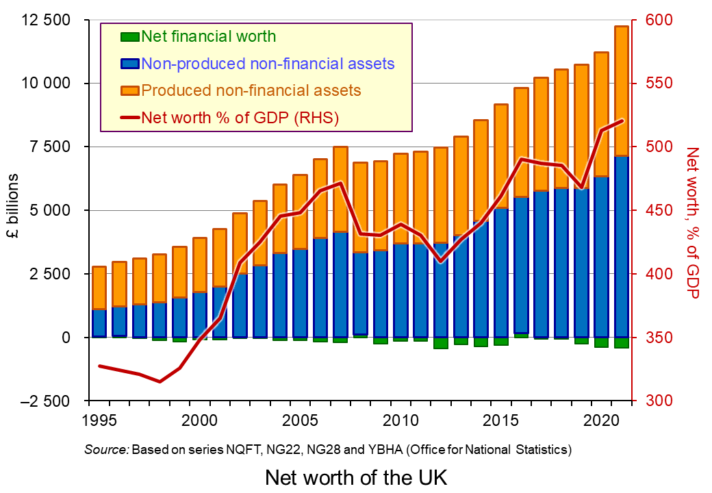 The chart shows the UK’s stock of net worth since 1995, alongside its value relative to annual national income (GDP) (click here for a PowerPoint). In 2021, the net worth of the UK was £11.8 trillion, equivalent to 5.2 times the country’s annual GDP. This marked an increase of £1.0 trillion or 9 per cent over 2020. This was driven largely by an increase in land values (non-produced non-financial assets).
In contrast, the stock of net worth fell in both 2008 and 2009 at the height of the financial crisis and the ensuing economic slowdown, which contributed to the country’s net worth falling by over 8 per cent.
The chart shows that net financial assets continue to make a negative contribution to the country’s net worth. In 2021 financial liabilities exceeded financial assets by the equivalent of 19 per cent of annual national income.
Non-financial corporations and the public sector together had financial liabilities in excess of financial assets of £3.4 trillion and £2.5 trillion respectively. However, once non-financial assets are accounted for, non-financial corporations had a positive net worth of £607 billion, although their value was not sufficient to prevent the public sector having a negative net worth of £1.2 trillion. Meanwhile, households had a positive net worth of £11.4 trillion and financial corporations a negative net worth of £4.9 billion.
Vulnerabilities and the balance sheets
The collapse of Silicon Valley Bank (SVB) resulted from balance sheet distress. Some argue that this distress can be attributed to a mismanagement of the bank’s liquidity position, which saw the bank use the surge in funds, on the back of buoyant activity among technology companies, to purchase long-dated bonds while, at the same time, reducing the share of assets held in cash. However, as the growth of the technology sector slowed as pandemic restrictions eased and, crucially, as central banks, including the Federal Reserve, began raising rates, the value of these long-dated bonds fell. This is because there is a negative relationship between interest rates and bond prices. Bonds pay a fixed rate of interest and so as other interest rates rise, bonds become less attractive to savers, pushing down their price. As depositors withdrew funds, Silicon Valley Bank found itself increasingly trying to generate liquidity from assets whose value was falling.
A major problem with balance sheet distress is contagion. This can occur, in part, because of what is known as ‘counterparty risk’. This simply refers to the idea that one party’s well-being is tied directly to that of another. However, the effects on economies from counterparty risks can be amplified by their impact on general credit conditions, confidence and uncertainty. This helps to explain why the US government stepped in quickly to guarantee SVB deposits.
There is, however, a ‘moral hazard’ problem here: if central banks are always prepared to step in, it can signal to banks that they are too big to fail and disincentivise them for adopting appropriate risk management strategies in the first place.
Subsequently, First Citizens Bank acquired the commercial banking business of SVB, while its UK subsidiary was acquired by HSBC for £1.
Interest rates and financial well-being
In light of the failures of SVB and Credit Suisse, the raising of interest rates by inflation-targeting central banks has raised concerns about the liquidity and liabilities positions of banks and non-bank financial institutions, such as hedge funds, insurers and pension funds. As we have seen, higher interest rates push down the value of bonds, which form a major part of banks’ balance sheets. The problem for central banks is that, if this forced them to make large-scale injections of liquidity by buying bonds (quantitative easing), it would make the fight against inflation more difficult. Quantitative easing is the opposite of tightening monetary policy and thus credit conditions, which are seen as necessary to control inflation.
 Yet the raising of interest rates has implications for the financial well-being of other sectors too since they also are affected by the effects on asset values and debt-servicing costs. For example, raising interest rates has a severe impact on the cashflow of UK homeowners with large variable-rate mortgages. This can substantially affect their spending. The UK has a high proportion of homeowners on variable-rate mortgages or fairly short-term fixed-rate mortgages. Also for a large number of households their mortgages are high relative to their incomes.
In short, falling asset values and increasing debt-servicing costs from rising interest rates in response to rising inflation tends to dampen spending in the economy. The effects will be larger the more burdened with debt people and businesses are, and the less liquidity they have to access. This has the potential to lead to a financial consolidation in order to restore the well-being of balance sheets. This involves cutting borrowing and spending.
Such a consolidation could be exacerbated if financial institutions become distressed and if it were to result in even larger numbers of people and businesses facing greater restrictions in accessing credit. These balance sheet pressures will continue to weigh on the policy responses of central banks as they attempt to navigate economies out of the current inflationary pressures.
Articles
Questions
- What is recorded on a balance sheet? Explain with reference to the household sector.
- What is meant by net worth? Does an increase in net worth mean that an individual’s or sector’s financial well-being has increased?
- What is meant by ‘liquidity-constrained’ individuals or businesses? What factors might explain how liquidity constraints arise?
- It is sometimes argued that there is a predator-prey relationship between income and debt. How could such a relationship arise and what is its importance for the economy?
- Why might a deterioration of a country’s balance sheets have both national and international consequences?
- Explain the possible trade-offs facing central banks when responding to inflationary pressures.
 The mandates of central banks around the world are typically focused on controlling inflation. In many cases, this is accompanied by operational independence from government, but with the government setting an inflation target. The central bank then chooses the appropriate monetary policy to achieve the inflation target. This is argued to provide the conditions that can deliver lower and less variable inflation rates – at least over the longer term.
However, some economists argue that this has the potential to create the conditions for greater economic volatility and financial instability. The events surrounding the collapse of Silicon Valley Bank (SVB) – the largest since the global financial crisis – have helped to reignite these debates.
Inflation targeting central banks
The theoretical foundations for delegating monetary policy to central banks with mandates to meet an inflation rate target is often attributed to the paper of Fynn Kydland and Edward Prescott published in the Journal of Political Economy in 1977. It argues that if governments, rather than independent central banks, operate monetary policy, systemically-high inflation can become established if low-inflation announcements by governments lack credibility. Delegation of monetary to a central bank with an inflation rate target, however, can create the necessary conditions for credibility. This, in turn, gives the public confidence to maintain lower and more stable inflationary expectations than would otherwise be the case.
To mitigate the problem of a potential inflationary bias, it is argued that governments should delegate monetary policy to a conservative central banker: one that places less weight on output or employment stabilisation and more weight on inflation stabilisation than does society. However, as identified by Kenneth Rogoff in his paper published in the Quarterly Journal of Economics in 1985, this raises the spectre of greater volatility in output and employment when economies are buffeted by supply shocks.
Inflation–output stabilisation trade-off
The inflation–output stabilisation trade-off identified by Rogoff has particular relevance to the macroeconomic environment experienced by many countries in recent times. As economies began to open up after the pandemic, demand–supply imbalances saw the 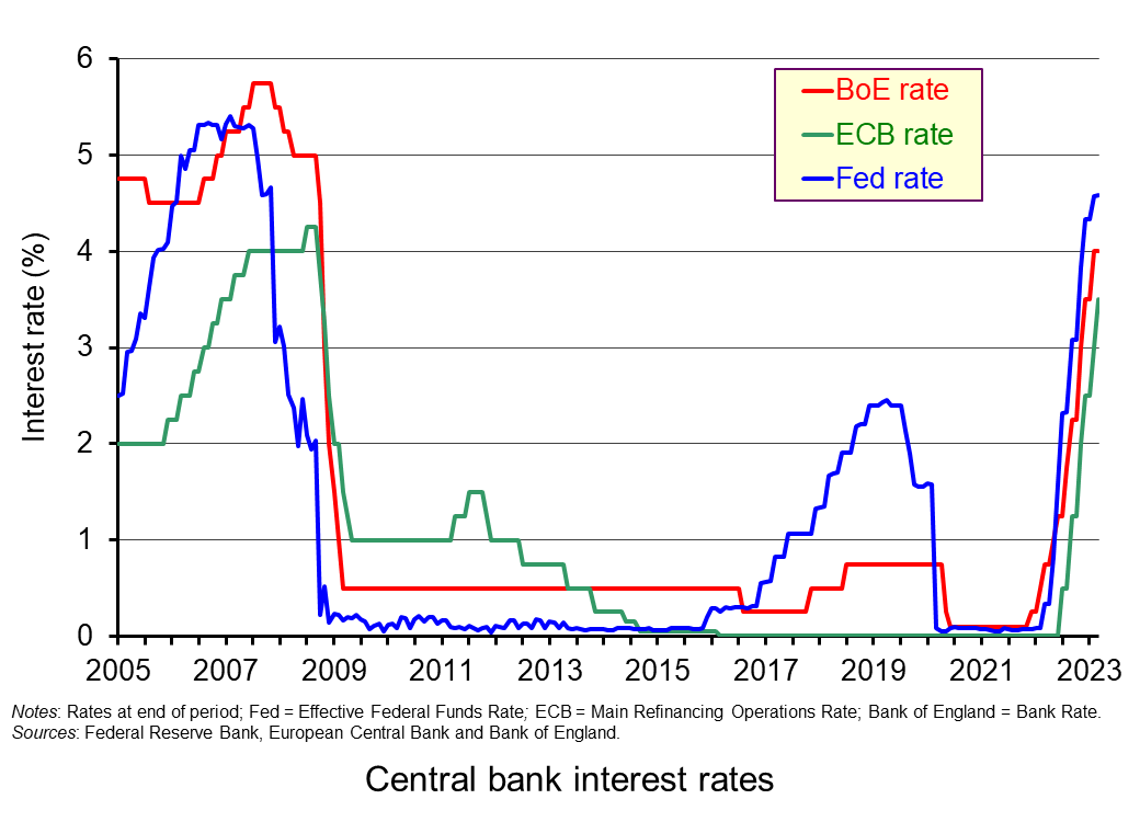 emergence of inflationary pressures. These pressures were then exacerbated by the Russian invasion of Ukraine, which drove up commodity prices.
Rather than pursuing a less contractionary policy in the face of these supply shocks so as to avoid recession, central banks stuck to their inflation mandates and hence raised interest rates significantly so as to bring inflation back to target as soon as possible. But this hampered economic recovery.
Inflation–financial stability trade-off
Yet the recent financial turmoil suggests a further inflation–stability trade-off: an inflation–financial stability trade-off. By raising interest rates, different sectors of the economy are liable to greater financial distress. This distress has contributed to the collapse of Silicon Valley Bank and Signature Bank, and led to a significant injection of funds by large US banks into First Republic. The fear is of a contagion within the financial sector, which then spills into other sectors of the economy.
The debate about central bank mandates and the weight attached to inflation stability relative to other objectives is therefore centre stage of macroeconomic policy debates.
Articles
- Inflation targeting and the 2 per cent goal
Financial Times, Editorial Board (16/12/22)
- Breaking the shackles of inflation targets
The Business Standard, Daniel Moss, Bloomberg (16/3/23)
- Evaluating Monetary Policy with Inflation Bands and Horizons
Federal Reserve Bank of San Francisco, letter, Troy Davig and Andrew Foerster (21/2/23)
- Need to rethink long-term inflation target: MPC member Ashima Goyal
The Economic Times (India) (15/3/23)
- Inflation Targeting Pros and Cons
Economicshelp, Tejvan Pettinger (16/11/17)
- Central banks walk tightrope in juggling mandates
Reuters, Mike Dolan (15/3/23)
- Silicon Valley Bank: why did it collapse and is this the start of a banking crisis?
The Guardian, Jonathan Barrett (13/3/23)
- Silicon Valley Bank: Regulators take over as failure raises fears
BBC News (11/3/23)
- HSBC swoops in to rescue UK arm of Silicon Valley Bank
BBC News, Michael Race (13/3/19)
- Silicon Valley Bank said it was too small to need regulation. Now it’s ‘too big to fail’
The Guardian, Rebecca Burns and Julia Rock (17/3/23)
- Multi-billion dollar rescue deal for First Republic Bank
BBC News, Natalie Sherman (16/3/19)
- Chancellor ‘welcomes’ decision to give Credit Suisse £44.5bn lifeline as shares bounce back
Sky News, Samuel Obsborne (16/3/23)
Questions
- Explain the argument that the delegation of monetary policy can help to keep the average rate of inflation lower.
- How might the monetary policy responses of central banks to an inflation shock create the possibility of an inflation–output stabilisation trade-off?
- What do you understand by a Taylor rule? Could this help to alleviate the inflation-output stabilisation trade-off?
- Some economists argue that there is less of a trade-off between inflation and output stability with demand-pull inflation because of a so-called ‘divine coincidence’ in monetary policy. Why might this be the case?
- What do you understand by the term ‘financial distress’? What metrics could be used to capture this for different sectors of the economy?
- Explain how financial contagion can spread both within and between different sectors of the economy.
 To make a sensible comparison of one year’s national income generated from the production of goods and services with another we need to take inflation into account. Changes in inflation-adjusted GDP represent changes in the volume of production of a country’s goods and services: in other words, the real value of goods and services. We revisit the blog written back in April 2019, prior the pandemic, to show how changes in real GDP evidence what we may refer to as the twin characteristics of economic growth: positive long-term growth but with fluctuating short-term rates of growth.
Real and nominal GDP
The nominal or current-price estimate for UK Gross Domestic Product in 2020 is £2.156 trillion. It is the value of output produced within the country in 2020. This was a fall of 4.4 per cent on the £2.255 trillion recorded in 2019. These values make no adjustment for inflation and therefore reflect the prices of output that were prevailing at the time.
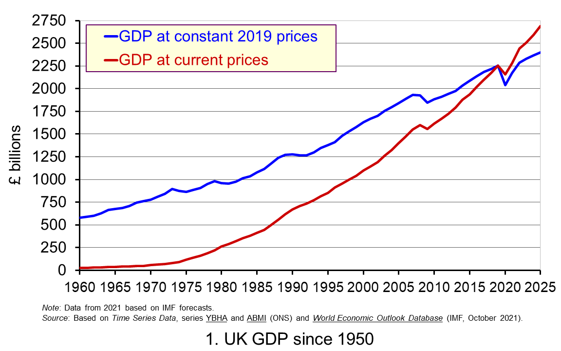 Chart 1 shows current-price estimates of GDP from 1950 when the value of GDP was estimated at £12.7 billion. The increase to £2.156 trillion in 2020 amounts to a proportionate increase of almost 170 times, a figure that rises to 211 times if we compare the 1950 value with the latest IMF estimate for 2025 of £2.689 trillion. However, if we want to make a more meaningful comparison of the country’s national income by looking at the longer-term increase in the volume of production, we need to adjust for inflation. (Click here to download a PowerPoint copy of the chart.)
Long-term growth in real GDP
If we measure GDP at constant prices, we eliminate the effect of inflation. To construct a constant-price series for GDP a process known as chain-linking is used. This involves taking consecutive pairs of years, e.g. 2020 and 2021, and estimating what GDP would be in the most recent year (in this case, 2021) if the previous year’s prices (i.e. 2020) had continued to prevail. By calculating the percentage change from the previous year’s GDP value we have an estimate of the volume change. If this is repeated for other pairs of years, we have a series of percentage changes that capture the volume changes from year-to-year. Finally, a reference year is chosen and the percentage changes are applied backwards and forwards from the nominal GDP value for the reference year – the volume changes forwards and backwards from this point.
In effect, a real GDP series creates a quantity measure in monetary terms. Chart 1 shows GDP at constant 2019 prices (real GDP) alongside GDP at current prices (nominal GDP). Consider first the real GDP numbers for 1950 and 2020. GDP in 1950 at 2019 prices was £410.1 billion. This is higher than the current-price value because prices in 2019 (the reference year) were higher than those in 1950. Meanwhile, GDP in 2020 when measured at 2019 prices was £2.037 trillion. This constant-price value is smaller than the corresponding current-price value because prices in 2019 where lower than those in 2020.
Between 1950 and 2020 real GDP increased 5.0 times. If we extend the period to 2025, again using the latest IMF estimates, the increase is 5.9 times. Because we have removed the effect of inflation, the real growth figure is much lower than the nominal growth figure. Crucially, what we are left with is an indicator of the long-term growth in the volume of the economy’s output and hence an increase in national income that is backed up by an increase in production. Whereas nominal growth rates are affected both by changes in volumes and prices, real growth rates reflect only changes in volumes.
The upward trajectory observed in constant-price GDP is therefore evidence of positive longer-term growth. This is one of the twin characteristics of growth.
Short-term fluctuations in the growth of real GDP
The second characteristic is fluctuations in the rate of growth from period to period. We can see this second characteristic more clearly by plotting the percentage change in real GDP from year to year.
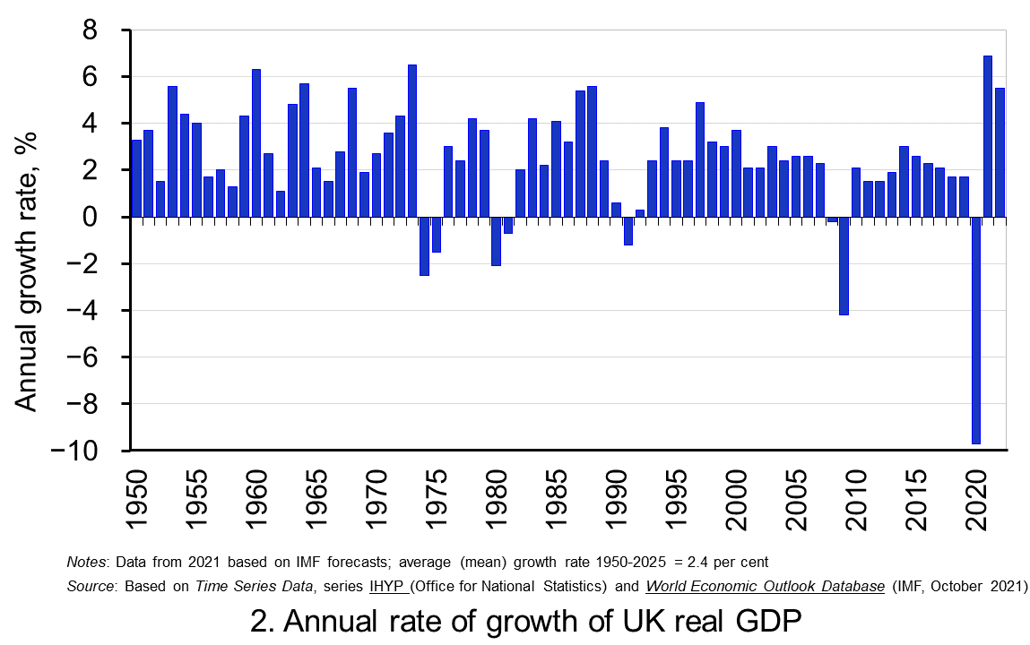 Chart 2 shows the annual rate of growth in real GDP each year since 1950. From it, we see the inherent instability that is a key characteristic of the macroeconomic environment. This instability is, of course, mirrored in the output path of real GDP in Chart 1, but the annual rates of growth show the instability more clearly. We can readily see the impact on national output of the global financial crisis and the global health emergency.
In 2009, constant-price GDP in the UK fell by 4.25 per cent. Then, in 2020, constant-price GDP and, hence, the volume of national output fell by 9.7 per cent, as compared to a 4.4 per cent fall in current-price GDP that we identified earlier. These global, ‘once-in-a-generation’ shocks are stark examples of the instability that characterises economies and which generate the ‘ups and downs’ in an economy’s output path, known more simply as ‘the business cycle’. (Click here to download a PowerPoint copy of the chart.)
Determinants of long-and short-term growth
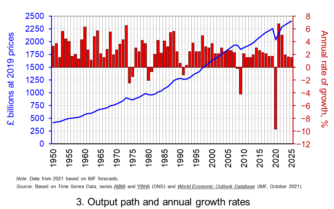 The twin characteristics of growth can be seen simultaneously by combining the output path captured by the levels of real GDP with the annual rates of growth. This is shown in Chart 3. The longer-term growth seen in the economy’s output path is generally argued to be driven by the quantity and quality of the economy’s resources, and their effectiveness when combined in production. In other words, it is the supply-side that determines the trajectory of the output path over the longer term. (Click here to download a PowerPoint copy of the chart.)
However, the fluctuations we observe in short-term growth rates tend to reflect impulses that affect the ability and or willingness of producers to supply (supply-side shocks) and purchasers to consume (demand-side shocks). These impulses are then propagated and their effects, therefore, transmitted through the economy.
Effects of the pandemic
The pandemic is unusual in that the health intervention measures employed by governments around the world resulted in simultaneous negative aggregate demand and aggregate supply shocks. Economists were particularly concerned that the magnitude of these impulses and their propagation had the potential to generate scarring effects and hence negative hysteresis effects. The concern was that these would affect the level of real GDP in the medium-to-longer term and, hence, the vertical position of the output path, as well as the longer-term rate of growth and, hence, the steepness of the output path.
The extent of these scarring effects continues to be debated. The ability of businesses and workers to adapt their practices, the extraordinary fiscal and monetary measures that were undertaken in many countries, and the roll-out of vaccines programmes, especially in advanced economies, have helped to mitigate some of these effects. For example, the latest IMF forecasts for output in the USA in 2024 are over 2 per cent higher than those made back in October 2019.
Scarring effects are, however, thought to be an ongoing issue in the UK. The IMF is now expecting output in the UK to be nearly 3 per cent lower than it originally forecast back in October 2019. Therefore, whilst UK output is set to recover, scarring effects on the UK economy will mean that the output path traced out by real GDP will remain, at least in the medium term, vertically lower than was expected before the pandemic.
Data and Reports
Articles
Questions
- What do you understand by the term ‘macroeconomic environment’? What data could be used to describe the macroeconomic environment?
- When a country experiences positive rates of inflation, which is higher: nominal economic growth or real economic growth?
- Does an increase in nominal GDP mean a country’s production has increased? Explain your answer.
- Does a decrease in nominal GDP mean a country’s production has decreased? Explain your answer.
- Why does a change in the growth of real GDP allow us to focus on what has happened to the volume of production?
- What does the concept of the ‘business cycle’ have to do with real rates of economic growth?
- When would falls in real GDP be classified as a recession?
- Distinguish between the concepts of ‘short-term growth rates’ and ‘longer-term growth’.
- What do you understand by the term hysteresis? By what means can hysteresis effects be generated?
- Discuss the proposition that the pandemic could have a positive effect on longer-term growth rates because of the ways that people and business have had to adapt.
 This is the second of three blogs looking at high inflation and its implications. Here we look at changes in the housing market and its effects on households. Another way of analysing the financial importance of the housing and mortgage markets is through the balance sheets and associated flow accounts of the household sector.
 Housing is also an important asset on household balance sheets. The price of housing reflects both the value of dwellings and the land on which they sit, and these are recorded separately on the balance sheets. Their combined balance sheet value increased from £1.09 trillion (£467.69bn + £621.49bn) in 1995 to £6.38 trillion (£1529.87bn + £4853.16bn) in 2021 or from 128% of GDP to 281%.
 The advent of higher interest rates was expected not only to impact on the debt servicing costs of households but the value of assets, including, in the context of this blog, housing. As Chart 3 in the previous blog helped to show, higher interest rates and higher mortgage repayments contributed to an easing of house price growth as housing demand eased. On the other hand, the impact on mortgaged landlords helped fuel the growth of rental prices as they passed on their increased mortgage repayment costs to tenants.
 This is the first of three blogs looking at inflation, at its effect on household budgets and at monetary policy to bring inflation back to the target rate. This first one takes an overview.
  Despite easing somewhat, the CPI inflation rate is showing signs of persistence – meaning that it is taking time for it to return to target. One way of understanding this persistence is to look at a measure of inflation known as core inflation. This inflation rate measure excludes energy, food, alcoholic beverages and tobacco prices, all of which are notoriously volatile. Core inflation thus captures underlying inflationary pressures.
 The increase in the Bank Rate is reflected in the increases in mortgage rates shown in Chart 2 (click
  Chart 3 provides a visual picture of the typical annual repayment costs facing first-time buyers as a percentage of earnings after tax and national insurance (click
  March 2023 saw the failure of Silicon Valley Bank (SVB), a regional US bank based in California that focused on financial services for the technology sector. It also saw the forced purchase of global-banking giant, Credit Suisse, by rival Swiss bank, UBS. These events fuelled concerns over the banking sector’s financial well-being, with fears for other financial institutions and the wider economy.
 A balance sheet is a record of stocks of assets and liabilities of individuals or organisations. Behind these stocks are accounts capturing flows, including income, expenditure, saving and borrowing. There are three types of flow accounts: income, financial and capital. Together, the balance sheets and flow accounts provide important insights into the overall financial position of individuals or organisations as well as the factors contributing to changes in their financial well-being.
 The chart shows the UK’s stock of net worth since 1995, alongside its value relative to annual national income (GDP) (click
  The mandates of central banks around the world are typically focused on controlling inflation. In many cases, this is accompanied by operational independence from government, but with the government setting an inflation target. The central bank then chooses the appropriate monetary policy to achieve the inflation target. This is argued to provide the conditions that can deliver lower and less variable inflation rates – at least over the longer term.
  emergence of inflationary pressures. These pressures were then exacerbated by the Russian invasion of Ukraine, which drove up commodity prices.
 To make a sensible comparison of one year’s national income generated from the production of goods and services with another we need to take inflation into account. Changes in inflation-adjusted GDP represent changes in the volume of production of a country’s goods and services: in other words, the real value of goods and services. We revisit the
  Chart 1 shows current-price estimates of GDP from 1950 when the value of GDP was estimated at £12.7 billion. The increase to £2.156 trillion in 2020 amounts to a proportionate increase of almost 170 times, a figure that rises to 211 times if we compare the 1950 value with the latest IMF estimate for 2025 of £2.689 trillion. However, if we want to make a more meaningful comparison of the country’s national income by looking at the longer-term increase in the volume of production, we need to adjust for inflation. (Click
  Chart 2 shows the annual rate of growth in real GDP each year since 1950. From it, we see the inherent instability that is a key characteristic of the macroeconomic environment. This instability is, of course, mirrored in the output path of real GDP in Chart 1, but the annual rates of growth show the instability more clearly. We can readily see the impact on national output of the global financial crisis and the global health emergency.
 The twin characteristics of growth can be seen simultaneously by combining the output path captured by the levels of real GDP with the annual rates of growth. This is shown in Chart 3. The longer-term growth seen in the economy’s output path is generally argued to be driven by the quantity and quality of the economy’s resources, and their effectiveness when combined in production. In other words, it is the supply-side that determines the trajectory of the output path over the longer term. (Click