 A previous post detailed how Netflix and Paramount Skydance were competing to acquire part or all of Warner Bros. Discovery (WBD). In December 2025, Netflix announced that it had agreed a deal to buy WBD’s studio and streaming service business. However, Paramount has still pursued a hostile takeover of WBD.
In mid-February 2026, it emerged that WBD had reopened talks with Paramount. Paramount was given a week to make its final offer. Then, under the agreed deal, Netflix would have the right to adjust its bid. Things have developed quickly since then.
Paramount raised its offer price by $1 per share making the deal worth a total of $111bn. WBD stated that this was superior to Netflix’s offer and Netflix declined to increase its bid. Netflix executives stated that:
This transaction was always a ‘nice to have’ at the right price, not a ‘must have’ at any price.1
Paramount will also pay Netflix the $2.8bn fee WBD owes Netflix for terminating the deal.
Whilst it appears Paramount has won the race to acquire WBD, the deal still needs regulatory clearance from competition authorities in the USA and Europe. Paramount CEO, David Ellison, stated that the proposal offered WBD shareholders ‘superior value, certainty and speed to closing.’2
Should the deal go through, the merged company would be in a powerful position as one of the few remaining Hollywood film and television studios.
References
- Paramount set for $111bn Warner Bros takeover after Netflix drops bid
BBC News, Danielle Kaye and Nardine Saad (26/2/26)
- Ibid
Articles
Questions
- What are the similarities and differences between Netflix’ and YouTube’s business models? How close substitutes do you think they are?
- Do you think cinemas are a closer or more distant substitute to Netflix than YouTube?
- Which of the possible deals, do you think, raised the most competition concerns? What might be a possible remedy that could alleviate these concerns?
- Was WBD’s decision to accept the Paramount takeover purely determined by the size of Paramount’s bid?
- What is the significance of legacy assets to the acquisition of WBD?
 Unemployment in the UK reached its highest level in nearly five years at the close of 2025, according to new data from the Office for National Statistics. Figures show the unemployment rate rising to 5.2% in the three months to December, up slightly from 5.1% in the preceding quarter.
This marks the highest unemployment level since the pandemic, coinciding with a slowdown in wage growth and increasing speculation that interest rates may soon be lowered.
Youth unemployment
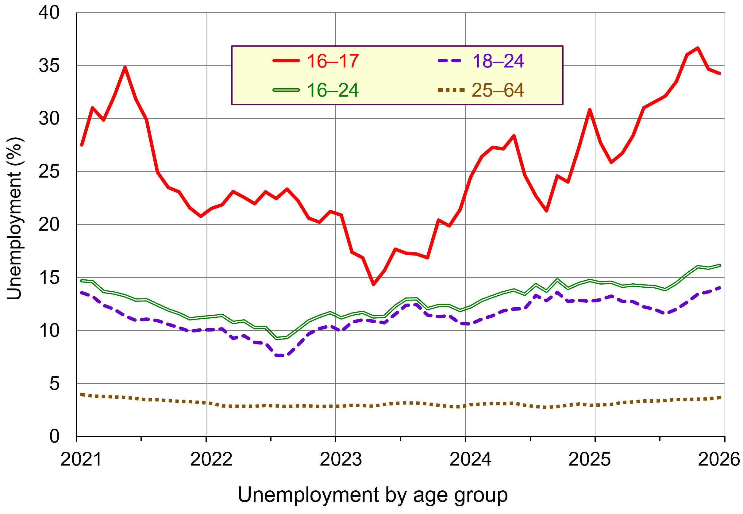 However, young people are taking the heaviest hit, with unemployment climbing to 16.1% among those aged 16 to 24. (Click here for a PowerPoint of the chart.) This is the highest level in more than a decade, including the spike seen during the pandemic. Economists largely attribute this trend to rising payroll costs, which they say are discouraging employers from offering entry level roles. Long-term youth unemployment is also worsening, with recent data showing that a growing share of unemployed young people have been out of work for over 12 months, highlighting deeper and more persistent barriers to re entry.
At the same time, although wages for those in work continue to grow faster than prices, the pace of wage growth is steadily slowing, adding further pressure on young people already facing the most challenging labour market conditions in years. According to ONS data, the annual growth in average weekly wages, excluding bonuses, slowed to 4.2% in the last three months of 2025. Private-sector wage growth eased to 3.4%, bringing it closer to the 3.25% rate that the Bank of England believes is consistent with its 2% inflation target.
The impact on interest rates
 The Bank of England is watching the slowdown in the UK jobs market closely as it gauges when next to lower its interest rates. In February 2026, the Monetary Policy Committee voted to hold the base rate (Bank Rate) at 3.75%. However, the committee voted with a majority of 5-4, with four members voting to reduce the rate to 3.5%.
The Bank of England uses interest rates as a policy tool to control inflation, the rate at which general prices rise in the economy. The current rate of inflation of 3.4% is above the Bank of England’s target of 2%.
In addition to the split vote, some economists believe that the easing in pay growth makes it likely that Bank Rate will be cut at the next meeting on 19th March. Paul Dales, chief UK economist at Capital Economics, said the fall in wage growth ‘supports the idea that the Bank of England has at least a couple more interest rate cuts in its locker’. A decrease in interest rates will be welcomed by investors.
What is behind the increase in youth unemployment?
Young people always tend to be the most impacted by a downturn in hiring. But economists warned that the rise in youth unemployment was a sign that employers are being more cautious about hiring younger workers. Openings for low-skilled entry-level roles and for new graduates have dropped steeply. Many businesses have slowed hiring due to an increase in costs because of measures in Chancellor Rachel Reeves’s last two Budgets. Businesses claim that the combination of increases in employer National Insurance contributions and a rise in the minimum wage mean they are facing higher payroll costs.
Peter Dixon at the National Institute for Economic and Social Research said, ‘there are indications that younger workers in particular are being priced out of the market’, supporting the explanation that raising the minimum wage might also be disincentivising the hiring of young people.
The ONS reported that the retail and wholesale sector saw the biggest fall in the number of workers on company payrolls, with 65,000 jobs lost in the sector since January last year. Meanwhile, health and social work saw the biggest rise in payrolled workers of any sector, adding 39,000 jobs in the year to January. Financial analyst at AJ Bell, Danni Hewson, suggested that those leaving the retail sector were now entering healthcare, with both sectors employing large numbers of women. However, she also warned that a recent surge in investment in artificial intelligence could hit young people the hardest as it could result ‘in a scarcity of entry level posts’ (see the blog Will AI make the world less equal?.
Job vacancies
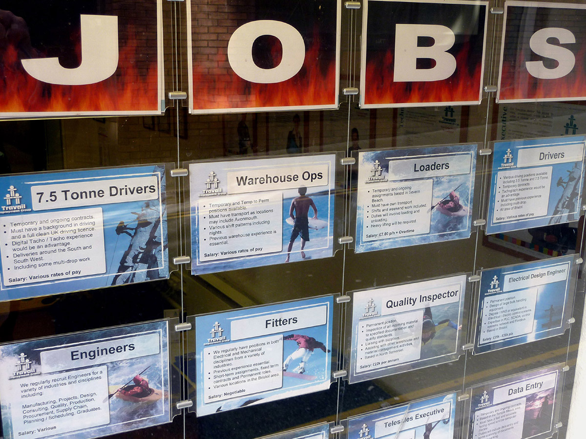 Job vacancy data across the UK indicates a significant cooling in labour demand. According to the latest ONS figures, vacancies fell from 736,000 in the three months to December to 726,000 in January, signalling continued weakening in hiring activity. According to the job search site, Adzuna, the number of vacant positions has dropped to its lowest level in five years, with job listings sliding 3% in January to 695,000, marking the first time vacancies have dipped below 700,000 since early 2021. Notably, graduate opportunities have fallen below 10,000 for the first time since Adzuna started tracking in 2016, underscoring the deepening challenges for new entrants to the workforce.
This downward trend in job openings extends patterns seen throughout late 2025, with vacancies down 16% from the previous January and nearly 20% lower than six months earlier. This coincides with a rise in unemployment to 5.2%, slower wage growth, and a growing concern that young people are disproportionately affected as hiring slows. As opportunities shrink, competition has intensified: there are now 2.4 jobseekers per vacancy, up from 2.27 in December, with the most sought-after roles including warehouse staff, healthcare support workers, lorry drivers, labourers and kitchen assistants.
How can the situation be improved?
Pat McFadden, Secretary for Work and Pensions, has commissioned the former Health Secretary Alan Milburn to lead a review into the causes of rising youth inactivity. There will be a particular focus on mental health issues that are pushing young people out of education and employment. This initiative responds to the growing number of young people not in education, employment, or training (NEETs), many of whom are now classified as inactive rather than unemployed. Some receive health-related benefits and are therefore not required to look for work, while others fall outside the benefits system entirely, making them harder to identify and support.
However, Pat McFadden said there was ‘more to do to get people into jobs’, and that tackling youth unemployment is a key government priority. He added that Labour was working to make it easier for young people to find and secure an apprenticeship, supported by a wider package of reforms. The reforms announced by McFadden include creating 50,000 additional apprenticeships. The government will also expand support for 350,000 people to move into work or training in sectors such as care and construction, with the risk of losing benefits if they refuse. They also include the provision of 55,000 state-funded, six-month work placements for the long-term unemployed.
While these measures are widely seen as necessary, campaign groups argue the government should go further by extending its ‘Youth Guarantee’ to cover all young people up to age 24, rather than ending at 22.
 However, as Alice Martin, head of research at Lancaster University’s Work Foundation, notes, initiatives designed to help people return to the labour market have limited impact ‘if the jobs aren’t out there.’ Even graduates are finding that opportunities are scarce, and for those leaving education with few qualifications, the situation is even more challenging. Sectors such as retail, once a reliable source of first jobs, have been in long-term structural decline, a trend that is now accelerating and further narrowing the pathways available to young people entering the workforce.
The situation has prompted government discussions about postponing the planned rise in the minimum wage for 18- to 20-year-olds to address employers’ concerns and encourage more youth employment. However, on Wednesday, Keir Starmer stressed that Labour remains committed to its manifesto pledge to align the pay of younger workers with that of older employees. The Prime Minister confirmed that the promise to ‘remove the discriminatory age bands’ in the minimum wage system still stands, and that the increase scheduled for April will proceed as planned.
Starmer said ‘We’ve made commitments to young people in our manifesto, and we will keep to those commitments, including the commitment that we would make sure that the living wage and minimum wage will go up this April, which we can absolutely confirm to you will happen.’
Unemployment outlook
Multiple economic forecasts predict that unemployment will to continue to rise in 2026. The most frequently cited projection places the 2026 unemployment rate around 5.2%–5.5%. However, some economists expect businesses to regain confidence and begin hiring again later in the year, supporting a gradual stabilisation in job markets.
Yet risks remain significant: if that recovery fails to materialise, unemployment could edge toward 6% by the end of the year, with forecasts from JP Morgan suggesting unemployment may reach 2 million in the first half as firms delay recruitment following the recent rise in the employers’ National Insurance rate. This environment is proving especially challenging for young people, with early career opportunities among the first to disappear and delayed entry into work potentially limiting long-term earnings and progression.
As hiring becomes more cautious and entry-level roles tighten, the path into the labour market risks becoming narrower, underscoring the need for policies and conditions that support both employer confidence and opportunities for new entrants.
Articles
FT Articles (subscribers only)
Data
Questions
- Explain why youth unemployment has risen more sharply than overall unemployment at the end of 2025.
- What are the costs to the individual of being unemployed?
- What are the wider non-monetary costs to society?
- Explain the main financial costs to the wider economy of a rising unemployment rate.
- Assess the likely impact of slowing wage growth on the Bank of England’s decision about whether or not to cut interest rates in early 2026.
- Discuss how falling job vacancies, particularly graduate and entry‑level opportunities, might affect long‑term labour market outcomes for young people.
- Evaluate the effectiveness of government policies such as expanding apprenticeships, increasing work placements, and reviewing youth inactivity in reducing youth unemployment.
 The television streaming market is currently attracting considerable attention from policy makers. This follows Warner Bros. accepting Netflix’s offer to buy part of the company for $72bn. To understand how this deal came about and why there is policy concern, we need to go back a few years.
The media and entertainment conglomerate Warner Bros. Discovery (WBD) was created in 2022 when AT&T sold Warner Bros to Discovery.1 However, in June 2025 the company announced that it would split the business into two parts. One would be (a) the studio for TV and movie production, where for example the Harry Potter franchises were made, and (b) the TV streaming business, home to for example the hit TV series Succession. The other, the more traditional and declining TV networks, including channels such as CNN, Discovery and TNT Sports, would form a new company called Discovery Global. David Zaslav, WBD President and Chief Executive stated that:
We are empowering these iconic brands with the sharper focus and strategic flexibility they need to compete most effectively in today’s evolving media landscape.2
Shortly afterwards, rival media and entertainment conglomerate, Paramount Skydance, made a series of bids to purchase the entire WBD business. But these were rejected by the WBD board. Despite this, in October 2025 WBD made public that it was open to a sale and had received unsolicited interest from several companies. It was believed that this included offers from Comcast and Netflix.
Recent developments
 In December 2025, Netflix announced that it had agreed a deal with WBD to buy its studio and streaming service business, including its back catalogue of shows. The deal is planned to be put to WBD shareholders in the next few months.3 Netflix has over 300m subscribers across the globe and streams popular shows, such as Stranger Things and Squid Games.
Despite this accepted offer, Paramount has subsequently pursued a hostile takeover of WBD by going straight to its shareholders. In addition, Paramount launched a lawsuit to get further information on how Netflix was chosen as the buyer and to provide WBD shareholders with information on the value of the TV network business that WBD was selling. This, however, was quickly thrown out of the courts.
Over time, Netflix and Paramount have tinkered with their bids to make them more attractive to WBD. Whilst Paramount’s bid was all cash, originally Netflix was offering a mixture of cash and shares. However, in January, it switched this to an all-cash offer. In February, Paramount made clear that if WBD instead accepted its offer, it would pay the $2.8bn termination fee that would be owed to Netflix.4 Furthermore, from early 2027 Paramount would pay WBD shareholders payments of $650m per quarter, known as ticking fees, if combining WBD and Paramount faced regulatory delay.
In mid-February 2026, it emerged that, following a waiver from Netflix, WBD had reopened talks with Paramount. Paramount was given a week to make its offer. Then, under the agreed deal, Netflix would have the right to adjust its bid. This is an attempt by WBD to end the hostile bidding war Paramount is pursuing and to provide clarity for its shareholders. WBD has reiterated that it will:
continue to recommend and remain fully committed to our transaction with Netflix. [However], we welcome the opportunity to engage with you and expeditiously determine whether Paramount Skydance can deliver an actionable, binding proposal that provides superior value.5
The insertion of the ticking fees by Paramount is in response to the substantial attention competition authorities across the globe are paying to the acquisition of WBD. The deal is being investigated by the US Department of Justice and, in early February, Netflix was questioned by the US Senate Antitrust Sub-committee. During this hearing, one of the Senators expressed his anger with the country’s competition laws and raised concerns that the deal would result in Netflix getting:
more power over consumers and leaving fewer alternatives and streaming platforms.6
While Paramount did not attend this hearing, it is believed that it has raised concerns about the Netflix-WBD deal to regulators. Netflix co-CEO, Ted Sarandos, has also met with Donald Trump to discuss the deal. However, Trump subsequently stated that the deal ‘could be a problem’.7
The EU and UK markets
 Furthermore, whilst all the companies involved are American, both the mergers with Netflix and Paramount are being investigated by the European Commission as markets in Europe would be affected.
In the UK, a group of politicians and former policymakers, have written to the Competition and Markets Authority urging it to conduct a full investigation of the Netflix-WBD merger. The letter argues that the merger could have:
damaging consequences for consumers, the UK’s world-leading creative industries and the UK cinema industry.
and that:
At a time when the British consumer can ill-afford more price increases, Netflix would possess an unprecedented ability to raise prices to access television and films.8
 The letter comes at a time when pressure is being placed on the CMA to adopt a generally more business-friendly approach.
The impact of the merger on the UK market is particularly complicated since Warner Bros.’ streaming service, HBO Max, is only due to launch in the UK in March 2026. This is still the plan, with WBD’s head of global streaming, Jean-Briac Perette acknowledging that:
We are likely the last scaled global streamer to come to market. We’ve tried to learn from the rest. We’re a complementary and distinct service to the more volume-driven or basic cable-like streamers in the market. More is not better. Better is better.9
An alternative route to regulatory approval
An easier route to regulatory approval may well be instrumental in allowing Netflix or Paramount to win the battle for WBD. Netflix stresses that the deal will create economic growth and jobs. Netflix’s Sarandos highlighted that:
This is not a typical media merger where you end up with what’s called the Noah’s Ark problem — two of everything. We are buying a company that has assets that we do not, and we will keep investing in those.10
The problem of economic power
In contrast, critics argue that either of the deals would create a new company with too much power. However, given the nature of the firms involved, the competition issues will be fundamentally different between the two deals.
 The Paramount deal would primarily reduce the number of studios in the market. This could provide the new merged studio with more bargaining power over distributors, advertisers and creators. Ultimately, this could negatively impact on the final product that consumers watch in the cinema and on television.
The Netflix deal on the other hand would impact directly on the streaming market. In the USA, 80% of consumers have both Netflix and HBO Max.11 After the merger, consumers would have less choice of competing services and Netflix-HBO Max combined may well have an incentive to raise its subscription prices.
In the UK, there are currently three leading streaming services: Netflix, Amazon Prime and Disney+, each with around 23% of the market.12 The merger with WBD could allow Netflix to become the clear market leader.
Concerns about YouTube
When examining streaming markets in all countries, an important factor will be whether to include YouTube in the market. Netflix certainly argues that it is a key competitor, at the hearing Sarandos stated that:
we are competing for the same content, we are competing for the same viewers, we are competing often for the same ad dollars. YouTube is not just cat videos anymore. YouTube is TV.13
If YouTube is included, in the USA it would be the market leader with 13%, ahead of Netflix on 9%. However, the competition authorities may conclude that YouTube’s product and business model is sufficiently different and so not include it in the streaming market.14
The issue of cinemas
 A second concern in the Netflix deal will be the Warner Bros.’ studio content that Netflix would own. The merged business may have an incentive to discontinue, raise the price or reduce the quality of the studio output that it supplies to cinemas. Thus, the competition authorities’ investigations will also pay close attention to the impact on the cinema market.
In line with these arguments, the Hollywood screenwriters’ union, the Writers Guild of America, has indicated that the Netflix-WMD deal should be stopped and filmmakers are clearly concerned about Netflix prioritising streaming.15
The competition authorities may well consider imposing remedies before they are willing to allow either deal to go ahead. With this in mind, it is interesting that Netflix has already made clear that it will continue the 45-day exclusive window that Warner Bros. provides cinemas to show its films.
It will be fascinating to see how the competing bids play out and how the competition regulators view them.
* * *
This post has been updated in a Postscript, following a further bid from Paramount that was not matched by Netflix.
References
- AT&T agrees deal to combine WarnerMedia with Discovery
The Guardian, Mark Sweney (16/5/21)
- HBO and CNN owner to split streaming and cable businesses
BBC News, Adam Hancock (10/6/25)
- Netflix’s co-CEO went to an antitrust hearing and a culture war broke out
NBC News, Saba Hamedy (3/2/26)
- Warner Bros gives Paramount seven days to make ‘best and final’ offer
The Guardian, Mark Sweney (17/2/26)
- ibid.
- NBC News, op. cit.
- Trump says $72bn Netflix-Warner Bros deal ‘could be a problem’
BBC News, Osmond Chia (8/12/25)
- UK politicians call for competition review of Netflix bid for Warner Bros
Financial Times (26/1/26)
- Warner streaming boss defends HBO Max UK launch ahead of Netflix takeover
Financial Times (9/2/26)
- NBC News, op. cit.
- Netflix and Warner Bros struggle to defend merger
BBC News, Danielle Kaye (3/2/26)
- Netflix, Disney+, Prime: Streaming platform market share report UK 2025
InsiderMedia, Jennifer O’Keeffe (2/12/25)
- BBC News, Danielle Kaye op. cit.
- Paramount sweetens Warner Bros bid with offer to pay Netflix break-up cost, other fees
Reuters, Harshita Mary Varghese and Aditya Soni (11/2/26)
- In a takeover of Warner Bros., Netflix makes a play for 21st century Hollywood’s throne
NBC News, Daniel Arkin (5/12/25)
Articles
Questions
- What are the similarities and differences between Netflix’ and YouTube’s business models? How close substitutes do you think they are?
- Do you think cinemas are a closer or more distant substitute to Netflix than YouTube?
- Which deal do you think raises the most competition concerns? What might be a possible remedy that could alleviate these concerns?
 At the fourth anniversary of Russia’s invasion of Ukraine, we look at the effect of the war on the Russian economy. Two years ago, in the blog The Russian economy after two years of war, we argued that the Russian economy had seemingly weathered the war successfully.
Unlike Ukraine, very little of its infrastructure had been destroyed; it had started the war with a current account balance of payments surplus, a budget surplus and a low general government debt-to-GDP ratio; it had achieved a lot of success in diverting its exports, including oil, away from countries imposing sanctions to countries such as China and India; it was the same with imports, with China especially becoming a major suppliers of machinery, components and vehicles; it has a strong central bank, which engenders a high level of confidence in managing inflation; the military expenditure provided a Keynesian boost to the economy, with production and employment rising.
The situation today
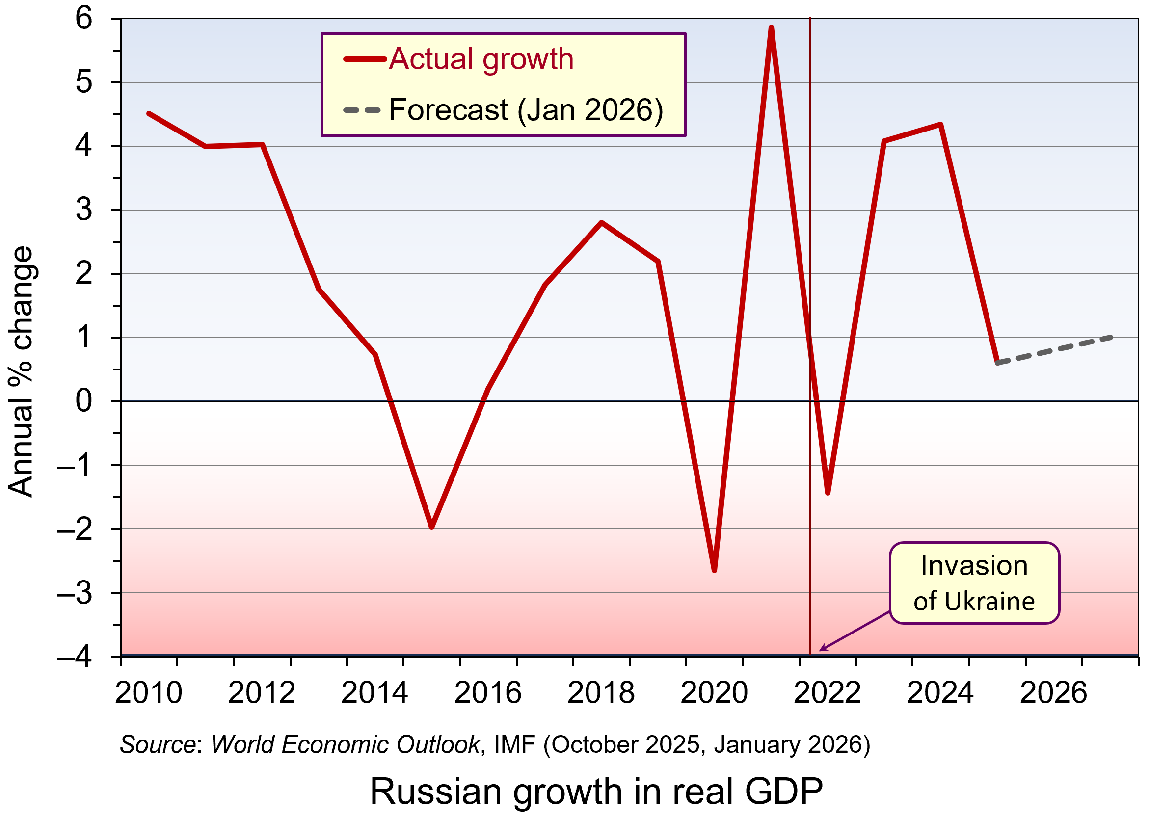 But two years further on, the Russian economy is looking a lot weaker and on the verge of recession. GDP growth fell to 0.6 per cent in 2025 and is forecast to be no more than 1 per cent for the next two years. (Click here for a PowerPoint of the chart.) And despite growth still being positive (just), this is largely because of the growth in military expenditure. Retail and wholesale trade fell by 1.1% in 2025, reflecting supply chain problems and high inflation dampening consumer demand.
With labour being diverted into the armaments and allied industries or into the armed forces, this has led to labour shortages. This has been compounded by the emigration of up to 1 million people by 2025 – often young, educated and skilled professionals.
 Official CPI inflation averaged 8.7 per cent in 2025, although the prices of food and other consumer essentials rose by more, especially in recent months. At the beginning of 2026, supermarket prices rose by 2.3% in just one month, made worse by a rise in VAT from 20% to 22%. The central bank has responded to the high inflation with high interest rates, which averaged 19.2% in 2025, giving a real rate of 10.5%. With such a high real rate, the response of households has been to save. This has masked the constraints on production, or imports, of consumer goods. Savings have also been boosted by large payments to soldiers and bereaved families, with the money saved by the recipients being used in part to fund future such payments. So far there has been trust in the banking system, but if that trust waned and people starting making large withdrawals of savings, it could be seriously destabilising.
Whilst the high real interest rates have helped to mask shortages of consumer goods, they have had a seriously dampening effect on investment by domestic companies. Gross capital formation fell by 3% in 2025, not helped by an increase in the corporation tax from 20% to 25%. At the same time, foreign direct investment remains subdued due to high perceived risks. The lack of investment, plus the labour shortages, will have profound effects on the supply side of the economy, with potential output in the non-military sector likely to decline over the medium term.
 The balance of payments and government finances are turning less favourable. The balance of trade surplus has declined from US$173bn in 2021 to US$67bn in 2025. This could decline further, or even become a deficit, if oil prices continue to be weak, if Western sanctions are tightened (such as stopping the flow of Russian oil exports in the ‘shadow’ fleet of tankers) or if major importing countries stop buying Russian oil. Indian refiners have announced that they are not taking Russian crude in March/April as India seeks to finalise a trade deal with the USA.
The budget balance has moved from a small surplus of 0.8% of GDP in 2021 to a deficit of 2.9% in 2025. Although the government debt-to-GDP ratio remains low by international standards at 23.1% of GDP in 2025, this was up from 16.5% in 2021 and is set to rise further as budget deficits deepen. Nevertheless, as long as the saving rate remains high, the debt can be serviced by domestic bond purchase.
Russia’s economy is definitely weakening and labour shortages and low investment will create major problems for the future. But whether this deterioration will be enough to change Russia’s stance on the war in Ukraine remains to be seen.
Articles
- The Russian economy is finally stagnating. What does it mean for the war – and for Putin?
The Guardian, Alex Clark (6/2/26)
- Exclusive: Russia’s budget deficit may almost triple this year as oil revenues decline
Reuters (4/2/26)
- Russia’s war economy is not collapsing, but neither is it stable
The Conversation, Yerzhan Tokbolat (17/12/25)
- Food prices are surging in Russia. Is the war hitting Russians in the pocket?
BBC News, Olga Shamina, Yaroslava Kiryukhina and Sergei Kagermazov (18/2/26)
- [Russian] GDP data — what it reveals, what it conceals
The Bell, Denis Kasyanchuk (18/2/26)
 What to Expect From the Russian Economy in 2026
Carnegie Endowment for International Peace, Alexandra Prokopenko and Alexander Gabuev (12/2/26)
- Indian refiners avoid Russian oil in push for US trade deal
Reuters, Nidhi Verma (8/2/26)
- What Breaks First – Russia’s Economy or Its War?
Visegrad Insight, Tomasz Kasprowicz (3/2/26)
Videos
Reports
Data
Questions
- What constraints are there currently on the supply side of the Russian economy?
- Some economists have argued that the economic effects of a stalemate in the Ukraine war would suit the Russian leadership more than peace or victory. Why might this be so?
- Under what circumstances might a deep recession in Russia be more likely than stagnation?
- In what ways does Russia’s current financial system resemble a pyramid scheme?
- What cannot a Keynesian boost contunue to support the Russian economy indefinitely?
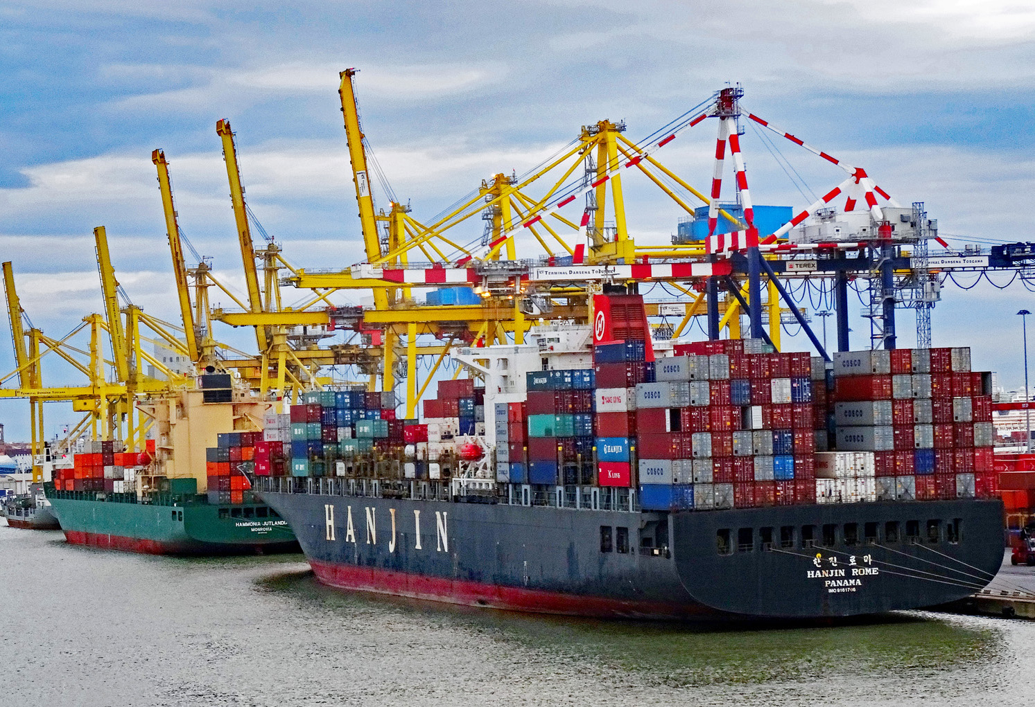 Three recent reports (see links below) have suggested that US consumers and businesses pay most of the tariffs imposed by the second Trump administration. The percentage varies from around 86% to 96%. US customs revenue surged by approximately $200 billion in 2025, but this was a tax paid almost entirely by US consumers and businesses. Foreign suppliers largely maintained their (pre-tariff) prices. They took a hit in terms of reduced volumes rather than reduced pre-tariff prices.
The incidence of a tariff between consumers, domestic importers and overseas producers will depend on price elasticities of demand and supply. The following diagram shows a product where the importing country is large enough to have a degree of market power, which will normally be the case with the USA. The greater its buying power, the flatter will be its demand curve, showing that the foreign supplier will have little influence on the price. With no tariff, the equilibrium price paid by importers will be at point a, where demand equals supply. Q1 would be imported at a price of P1.
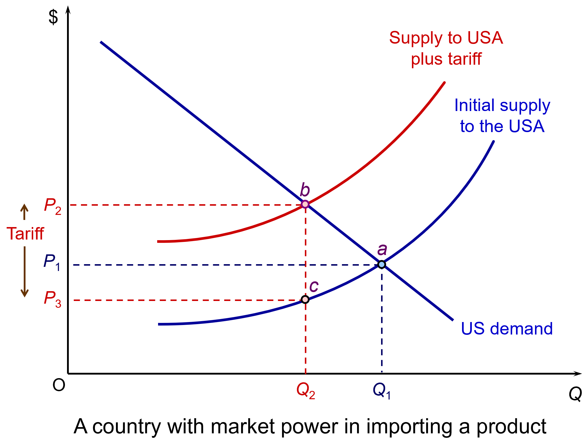 Imposition of a tariff will shift the supply curve upwards by the amount of the tariff. The new equilibrium price paid by importers will be at point b, where the new supply curve crosses the demand curve. Importers thus now pay a post-tariff price of P2: an effective rise in price of P2 minus P1. Foreign exporters receive P3, which is what they are paid by importers after the tariff has been paid.
The consumer price will be above P2 as that includes a mark-up by US businesses on top of the price they pay to import the product. Importers may bear some of the increase in price and not pass the full amount onto consumers, depending on competition and their ability to absorb cost increases.
President Trump argued that there would be very little rise in price from the tariffs and that overseas suppliers would bear the brunt of the tariffs. Indeed, recently he has argued that this must be the case as US inflation has been falling. In response, critics maintain that the rate of inflation would have fallen more without the tariffs and that current prices would be lower than they are. Also, if US importing firms or retailers bear some of the increased cost, even though this helps to dampen the price rise, their lower profits could damage investment and employment.

The Reports
The first report is from the New York Fed (one of the regional branches of the Federal Reserve Bank). It examines the effect of tariffs imposed in 2025, over three periods: (i) January to August, (ii) September to October, and (iii) November. In the first period, 94% of the tariffs were paid by US importers and 6% by foreign exports; in the second period, the figures were 92% and 8% and in the third period, 86% and 14%.
The second report is The Budget and Economic Outlook: 2026 to 2036 from the Congressional Budget Office. Box 2-1 notes that, as of November 2025, ‘the effective tariff rate was about 13 percentage points higher than the roughly 2 percent rate on imports in 2024’. Its analysis suggests that 95% of the tariffs will be borne by importers. Of these higher import prices, 30% will be borne by US businesses, largely through reduced profit margins, and 70% by consumers through higher prices. This will also allow many businesses which produce goods that compete with foreign imports to ‘increase their prices because of the decline in competition from abroad and the increased demand for tariff-free domestic goods’.
The third report is from the Kiel Insitut. In its Policy Brief, Americaʼs Own Goal: Who Pays the Tariffs?, it finds that US importers and consumers bear 96% of the cost of the 2025 tariffs, with foreign exporters absorbing only about 4%. It bases it findings on shipment-level data covering over 25 million transactions valued at nearly $4 trillion. This also shows that exports to the USA declined as foreign exporters preferred to reduce volumes rather than absorbing the tariffs.
The tariffs raised some $200 billion in 2025, around 3.8% of Federal tax receipts. But, as we have seen, this was paid largely by US consumers and business. It goes some way to offsetting the annual cut in tax revenues of around $450 to $520 billion per year from the tax cuts, largely to the better off, in Trump’s ‘One Big Beautiful Bill’.
Reports
Aricles
- NY Fed report says Americans pay for almost all of Trump’s tariffs
Reuters, Michael S. Derby (12/2/25)
- A year in, it’s official: Americans, not foreigners, are paying for Trump’s tariffs
CNN, Allison Morrow (12/2/26)
- Costs from Trump’s tariffs paid mainly by US firms and consumers, NY Fed says
BBC News, Kali Hays (13/2/26)
- Consumers and businesses paid nearly 90% of Trump tariffs in 2025, new analysis found
CBS News, Megan Cerullo (12/2/26)
- New Studies Challenge Who Really Pays for Tariffs
Investopedia, Diccon Hyatt (12/2/26)
- Trump Tariffs: Tracking the Economic Impact of the Trump Trade War
Tax Foundation, Erica York and Alex Durante (6/2/26)
- Who Is Paying the Trump Tariffs?
Paul Krugman (15/2/26)
Questions
- Summarise the findings of the three reports (but just Box 2-1 of the Congressional Budget Office one).
- Assess the argument that protectionism leads to inefficiency in the protected industries.
- Under what circumstances would exporters to the USA absorb a high percentage of tariff increases? Consider questions of elasticity.
- Can tariffs ever be justified on efficiency grounds?
- Can tariffs be justified as a bargaining ploy? Can they be used as a means of achieving freer and fairer trade?
- Read the blog, President Reagan on tariffs and summarise President Reagan’s arguments. Are they still relevant today?
- Consider the arguments for and against the EU raising tariffs on US goods.
 A previous post detailed how Netflix and Paramount Skydance were competing to acquire part or all of Warner Bros. Discovery (WBD). In December 2025, Netflix announced that it had agreed a deal to buy WBD’s studio and streaming service business. However, Paramount has still pursued a hostile takeover of WBD.
  Unemployment in the UK reached its highest level in nearly five years at the close of 2025, according to new data from the Office for National Statistics. Figures show the unemployment rate rising to 5.2% in the three months to December, up slightly from 5.1% in the preceding quarter.
 However, young people are taking the heaviest hit, with unemployment climbing to 16.1% among those aged 16 to 24. (Click
  The Bank of England is watching the slowdown in the UK jobs market closely as it gauges when next to lower its interest rates. In February 2026, the Monetary Policy Committee voted to hold the base rate (Bank Rate) at 3.75%. However, the committee voted with a majority of 5-4, with four members voting to reduce the rate to 3.5%.
  Job vacancy data across the UK indicates a significant cooling in labour demand. According to the latest ONS figures, vacancies fell from 736,000 in the three months to December to 726,000 in January, signalling continued weakening in hiring activity. According to the job search site, Adzuna, the number of vacant positions has dropped to its lowest level in five years, with job listings sliding 3% in January to 695,000, marking the first time vacancies have dipped below 700,000 since early 2021. Notably, graduate opportunities have fallen below 10,000 for the first time since Adzuna started tracking in 2016, underscoring the deepening challenges for new entrants to the workforce.
 However, as Alice Martin, head of research at Lancaster University’s Work Foundation, notes, initiatives designed to help people return to the labour market have limited impact ‘if the jobs aren’t out there.’ Even graduates are finding that opportunities are scarce, and for those leaving education with few qualifications, the situation is even more challenging. Sectors such as retail, once a reliable source of first jobs, have been in long-term structural decline, a trend that is now accelerating and further narrowing the pathways available to young people entering the workforce.
 In December 2025, Netflix announced that it had agreed a deal with WBD to buy its studio and streaming service business, including its back catalogue of shows. The deal is planned to be put to WBD shareholders in the next few months.3 Netflix has over 300m subscribers across the globe and streams popular shows, such as Stranger Things and Squid Games.
  Furthermore, whilst all the companies involved are American, both the mergers with Netflix and Paramount are being investigated by the European Commission as markets in Europe would be affected.
 The letter comes at a time when pressure is being placed on the CMA to adopt a generally more business-friendly approach.
  The Paramount deal would primarily reduce the number of studios in the market. This could provide the new merged studio with more bargaining power over distributors, advertisers and creators. Ultimately, this could negatively impact on the final product that consumers watch in the cinema and on television.
  A second concern in the Netflix deal will be the Warner Bros.’ studio content that Netflix would own. The merged business may have an incentive to discontinue, raise the price or reduce the quality of the studio output that it supplies to cinemas. Thus, the competition authorities’ investigations will also pay close attention to the impact on the cinema market.
  At the fourth anniversary of Russia’s invasion of Ukraine, we look at the effect of the war on the Russian economy. Two years ago, in the blog
  But two years further on, the Russian economy is looking a lot weaker and on the verge of recession. GDP growth fell to 0.6 per cent in 2025 and is forecast to be no more than 1 per cent for the next two years. (Click
  Official CPI inflation averaged 8.7 per cent in 2025, although the prices of food and other consumer essentials rose by more, especially in recent months. At the beginning of 2026, supermarket prices rose by 2.3% in just one month, made worse by a rise in VAT from 20% to 22%. The central bank has responded to the high inflation with high interest rates, which averaged 19.2% in 2025, giving a real rate of 10.5%. With such a high real rate, the response of households has been to save. This has masked the constraints on production, or imports, of consumer goods. Savings have also been boosted by large payments to soldiers and bereaved families, with the money saved by the recipients being used in part to fund future such payments. So far there has been trust in the banking system, but if that trust waned and people starting making large withdrawals of savings, it could be seriously destabilising.
 The balance of payments and government finances are turning less favourable. The balance of trade surplus has declined from US$173bn in 2021 to US$67bn in 2025. This could decline further, or even become a deficit, if oil prices continue to be weak, if Western sanctions are tightened (such as stopping the flow of Russian oil exports in the ‘shadow’ fleet of tankers) or if major importing countries stop buying Russian oil. Indian refiners have announced that they are not taking Russian crude in March/April as India seeks to finalise a trade deal with the USA.
  Three recent reports (see links below) have suggested that US consumers and businesses pay most of the tariffs imposed by the second Trump administration. The percentage varies from around 86% to 96%. US customs revenue surged by approximately $200 billion in 2025, but this was a tax paid almost entirely by US consumers and businesses. Foreign suppliers largely maintained their (pre-tariff) prices. They took a hit in terms of reduced volumes rather than reduced pre-tariff prices.
 Imposition of a tariff will shift the supply curve upwards by the amount of the tariff. The new equilibrium price paid by importers will be at point b, where the new supply curve crosses the demand curve. Importers thus now pay a post-tariff price of P2: an effective rise in price of P2 minus P1. Foreign exporters receive P3, which is what they are paid by importers after the tariff has been paid.