 The Institute of Fiscal Studies (IFS) has just published its annual ‘Green Budget‘. This is, in effect, a pre-Budget report (or a substitute for a government ‘Green Paper’) and is published ahead of the government’s actual Budget.
The Green Budget examines the state of the UK economy, likely economic developments and the implications for macroeconomic policy. This latest Green Budget is written in the context of Brexit and the growing likelihood of a hard Brexit (i.e. a no-deal Brexit). It argues that the outlook for the public finances has deteriorated substantially and that the economy is facing recession if the UK leaves the EU without a deal.
It predicts that:
Government borrowing is set to be over £50 billion next year (2.3% of national income), more than double what the OBR forecast in March. This results mainly from a combination of spending increases, a (welcome) change in the accounting treatment of student loans, a correction to corporation tax revenues and a weakening economy. Borrowing of this level would breach the 2% of national income ceiling imposed by the government’s own fiscal mandate, with which the Chancellor has said he is complying.
A no-deal Brexit would worsen this scenario. The IFS predicts that annual government borrowing would approach £100 billion or 4% of GDP. National debt (public-sector debt) would rise to around 90% of GDP, the highest for over 50 years. This would leave very little scope for the use of fiscal policy to combat the likely recession.
The Chancellor, Sajid Javid, pledged to increase public spending by £13.4bn for 2020/21 in September’s Spending Review. This was to meet the Prime Minister’s pledges on increased spending on police and schools. This should go some way to offset the dampening effect on aggregate demand of a no-deal Brexit. The government has also stated that it wishes to cut various taxes, such as increasing the threshold at which people start paying the 40% rate of income tax from £50 000 to £80 000. But even with a ‘substantial’ fiscal boost, the IFS expects little or no growth for the two years following Brexit.
 But can fiscal policy be used over the longer term to offset the downward shock of Brexit, and especially a no-deal Brexit? The problem is that, if the government wishes to prevent government borrowing from soaring, it would then have to start reining in public spending again. Another period of austerity would be likely.
There are many uncertainties in the IFS predictions. The nature of Brexit is the obvious one: deal, no deal, a referendum and a remain outcome – these are all possibilities. But other major uncertainties include business and consumer sentiment. They also include the state of the global economy, which may see a decline in growth if trade wars increase or if monetary easing is ineffective (see the blog: Is looser monetary policy enough to stave off global recession?).
Articles
IFS Report
Data
Questions
- Why would a hard Brexit reduce UK economic growth?
- To what extent can expansionary fiscal policy stave off the effects of a hard Brexit?
- Does it matter if national debt (public-sector debt) rises to 90% or even 100% of GDP? Explain.
- Find out the levels of national debt as a percentage of GDP of the G7 countries. How has Japan managed to sustain such a high national debt as a percentage of GDP?
- How can an expansionary monetary policy make it easier to finance the public-sector debt?
- How has investment in the UK been affected by the Brexit vote in 2016? Explain.
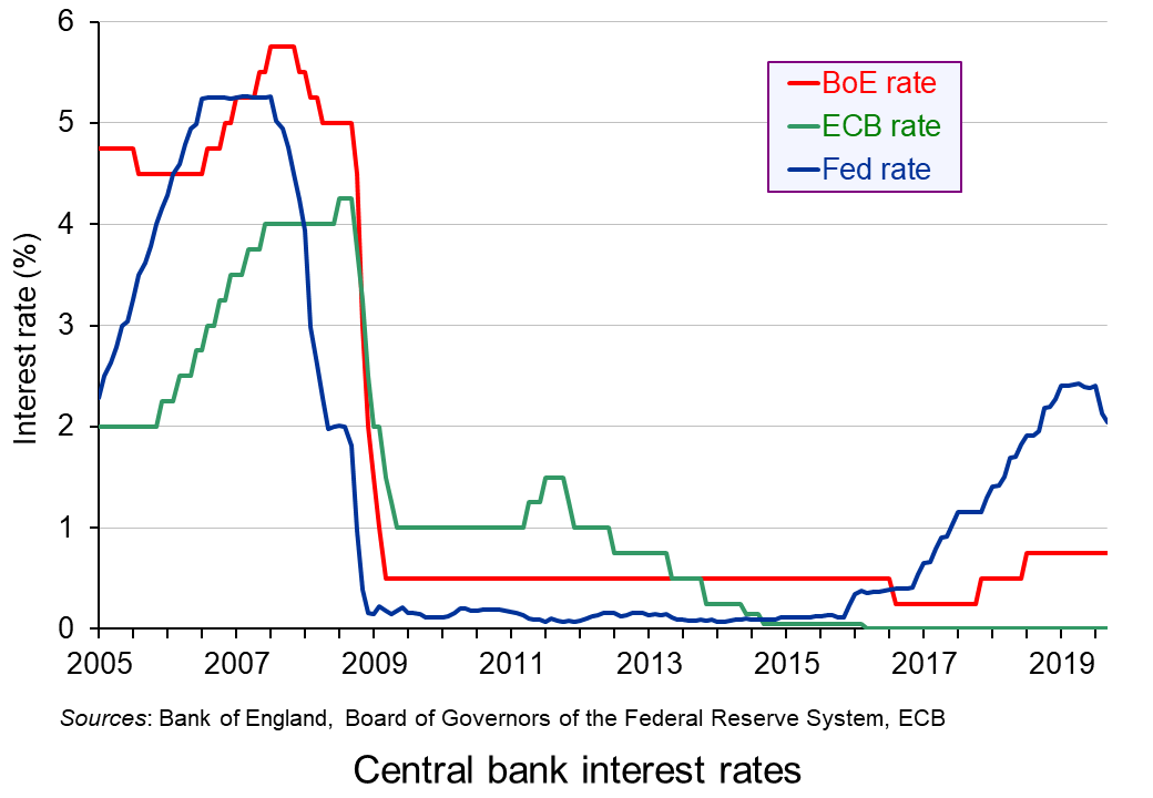
 With the prospects of weaker global economic growth and continuing worries about trade wars, central banks have been loosening monetary policy. The US central bank, the Federal Reserve, lowered its target Federal Funds rate in both July and September. Each time it reduced the rate by a quarter of a percentage point, so that it now stands at between 1.75% and 2%.
The ECB has also cut rates. In September it reduced the overnight deposit rate for banks from –0.4% to –0.5%, leaving the main rate at 0%. It also introduced a further round of quantitative easing, with asset purchases of €20 billion per month from 1 November and lasting until the ECB starts raising interest rates.
The Australian Reserve Bank has cut its ‘cash rate‘ three times this year and it now stands at an historically low level of 0.75%. Analysts are predicting that it may be forced to introduce quantitative easing if lower interest rates fail to stimulate growth.
Japan continues with its programme of quantitative easing (QE) and other central banks are considering lowering interest rates and/or (further) QE.
 But there are two key issues with looser monetary policy.
The first is whether it will be sufficient to provide the desired stimulus. With interest rates already at or near historic lows (although slightly above in the case of the USA), there is little scope for further reductions. QE may help, but without a rise in confidence, the main effect of the extra money may simply be a rise in the price of assets, such as property and shares. It may result in very little extra spending on consumption and investment – in other words, very little extra aggregate demand.
The second is the effect on inequality. By inflating asset prices, QE rewards asset owners. The wealthier people are, the more they will gain.
Many economists and commentators are thus calling for the looser monetary policy to be backed up by expansionary fiscal policy. The boost to aggregate demand, they argue, should come from higher public spending, with governments able to borrow at very low interest rates because of the loose monetary policy. Targeted spending on infrastructure would have a supply-side benefit as well as a demand-side one.
Articles
- European Central Bank cuts its deposit rate, launches new bond-buying program
CNBC, Elliot Smith (12/9/19)
- Can monetary policies help prevent a global recession?
Investment Week, Martin Gilbert (7/10/19)
- Draghi’s Utmost Is Still Not Enough
Bloomberg, John Authers (13/9/19)
- Draghi puts heat on politicians to boost fiscal stimulus with his ECB swan song
MarketWatch, William Watts (12/9/19)
- To infinity and beyond: ECB’s quantitative easing
EJ Insight, Raphael Olszyna-Marzys (2/10/19)
- The dangers of negative interest rates
Money Week, Merryn Somerset Webb (7/10/19)
- Schwarzman: Europe could enter Japan-style stagnation if governments don’t start spending
CNBC, Elliot Smith (7/10/19)
- US Fed cuts interest rates for second time since 2008
BBC News, Andrew Walker (18/9/19)
- Current Federal Reserve Interest Rates and Why They Change
The Balance, Kimberly Amadeo (19/9/19)
- Federal Reserve Interest Rate Cuts Alone Can’t Prevent a Recession
Barron’s, Al Root (4/10/19)
- Why is the Fed pumping money into the banking system?
BBC News, Natalie Sherman (19/9/19)
- Top of Lagarde’s ECB to-do list: stop QE and democratise monetary policy
Social Europe, Jens van’t Klooster (25/9/19)
- Economists warn Reserve Bank could be forced to print money if rate cuts fail to deliver
The Guardian, Martin Farrer (2/10/19)
- A very large gamble: evidence on Quantitative Easing in the US and UK
Institute for Policy Research. Policy Brief, Chris Martin and Costas Milas
- The verdict on 10 years of quantitative easing
The Guardian, Richard Partington (8/3/19)
ECB Press Conference
Questions
- Explain what is meant by quantitative easing.
- What determines the effectiveness of quantitative easing?
- Why is President Trump keen for the Federal Reserve to pursue more aggressive interest rate cuts?
- What is the Bank of England’s current attitude towards changing interest rates and/or further quantitative easing?
- What are the current advantages and disadvantages of governments pursuing a more expansionary fiscal policy?
- Compare the relative merits of quantitative easing through asset purchases and the use of ‘helicopter money’.
 It’s been a while since I last blogged about labour markets and, in particular, about the effect of automation on wages and employment. My most recent post on this topic was on the 14th of April 2018 and it was mostly a reflection on some interesting findings that had been reported by Acemoglu et al (2017). More specifically, Acemoglu and Restrepo (2017) developed a theoretical framework to evaluate the effect of AI on employment and wages. They concluded that the effect was negative and potentially sizeable (for a more detailed discussion see my blog).
Using a model in which robots compete against human labor in the production of different tasks, we show that robots may reduce employment and wages … According to our estimates, one more robot per thousand workers reduces the employment to population ratio by about 0.18–0.34 percentage points and wages by 0.25–0.5 percent.
Since then, I have seen a constant stream of news on my news feed about the development of ever more advanced industrial robots and artificial intelligence. And this was not because of some spooky coincidence (or worse). It has been merely a reflection of the speed at which technology has been progressing in this field.
There are now robots that can run, jump, hold conversations with humans, do gymnastics (and even sweat for it!) and more. It is really impressive how fast change has been happening recently in this field – and, unsurprisingly, it has stimulated the interest of labour economists!
A paper that has recently come to my attention on this subject is by Graetz and Michaels (2018). The authors put together a panel dataset on robot adoption within seventeen countries from 1993 to 2007 and use advanced econometric techniques to evaluate the effect of these technologies on employment and productivity growth. Their analysis focuses exclusively on developed economies (due to data limitations, as they explain) – but their results are nevertheless intriguing:
We study here for the first time the relationship between industrial robots and economic outcomes across much of the developed world. Using a panel of industries in seventeen countries from 1993 to 2007, we find that increased use of industrial robots is associated with increases in labor productivity. We find that the contribution of increased use of robots to productivity growth is substantial and calculate using conservative estimates that it comes to 0.36 percentage points, accounting for 15% of the aggregate economy-wide productivity growth.
The pattern that we document is robust to including various controls for country trends and changes in the composition of labor and other capital inputs. We also find that robot densification is associated with increases in both total factor productivity and wages, and reductions in output prices. We find no significant relationship between the increased use of industrial robots and overall employment, although we find that robots may be reducing the employment of low-skilled workers.
This is very positive news for most – except, of course, for low-skilled workers. Indeed, like Acemoglu and Restrepo (2017) and many others, this study shows that the effect of automation on employment and labour market outcomes is unlikely to be uniform across all types of workers. Low-skilled workers are found again to be likely to lose out and be significantly displaced by these technologies.
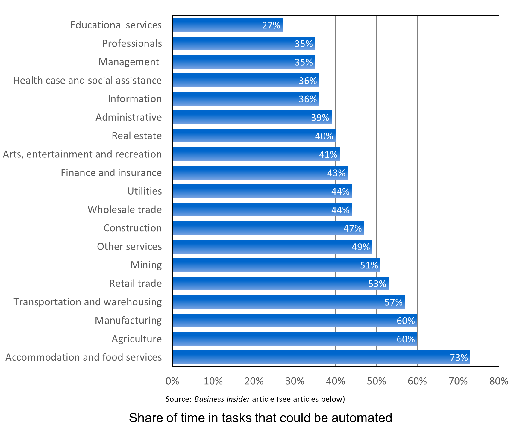
And if you are wondering which sectors are likely to be disrupted most/first by automation, the rankings developed by McKinsey and Company (see chart below) would give you an idea of where the disruption is likely to start. Unsurprisingly, the sectors that seem to be the most vulnerable, are the ones that use the highest share of low-skilled labour.
Articles
Questions
- “The effect of automation on wages and employment is likely to be positive overall”. Discuss.
- Using examples and anecdotal evidence, do you agree with these findings?
- Using Google Scholar, put together a list of 5 recent (i.e. 2015 or later) articles and working papers on labour markets and automation. Compare and discuss their findings.
 Donald Trump has suggested that the Fed should cut interest rates by 1 percentage point and engage in a further round of quantitative easing. He wants to see monetary policy used to give a substantial boost to US economic growth at a time when inflation is below target. In a pair of tweets just before the meeting of the Fed to decide on interest rates, he said:
China is adding great stimulus to its economy while at the same time keeping interest rates low. Our Federal Reserve has incessantly lifted interest rates, even though inflation is very low, and instituted a very big dose of quantitative tightening. We have the potential to go up like a rocket if we did some lowering of rates, like one point, and some quantitative easing. Yes, we are doing very well at 3.2% GDP, but with our wonderfully low inflation, we could be setting major records &, at the same time, make our National Debt start to look small!
But would this be an appropriate policy? The first issue concerns the independence of the Fed.
It is supposed to take decisions removed from the political arena. This means sticking to its inflation target of 2 per cent over the medium term – the target it has officially had since January 2012. To do this, it adjusts the federal funds interest rate and the magnitude of any bond buying programme (quantitative easing) or bond selling programme (quantitative tightening).
The Fed is supposed to assess the evidence concerning the pressures on inflation (e.g. changes in aggregate demand) and what inflation is likely to be over the medium term in the absence of any changes in monetary policy. If the Federal Open Market Committee (FOMC) expects inflation to exceed 2 per cent over the medium term, it will probably raise the federal funds rate; if it expects inflation to be below the target it will probably lower the federal funds rate.
In the case of the economy being in recession, and thus probably considerably undershooting the target, it may also engage in quantitative easing (QE). If the economy is growing strongly, it may sell some of its portfolio of bonds and thus engage in quantitative tightening (QT).
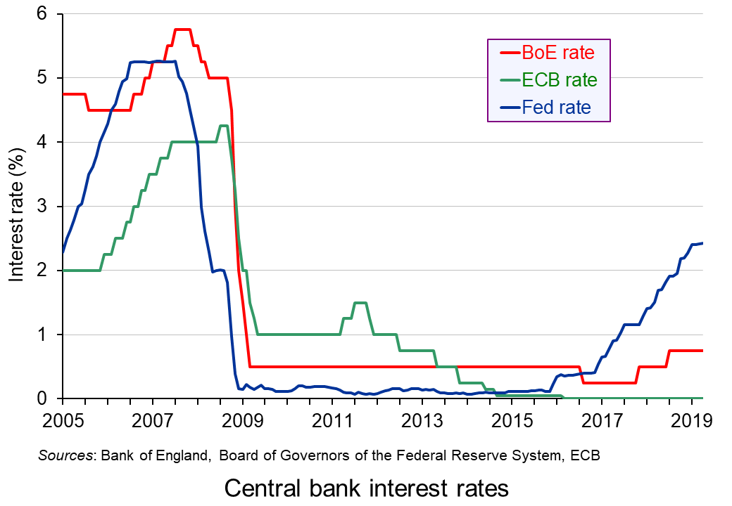 Since December 2015 the Fed has been raising interest rates by 0.25 percentage points at a time in a series of steps, so that the federal funds rate stands at between 2.25% and 2.5% (see chart). And since October 2017, it has also been engaged in quantitative tightening. In recent months it has been selling up to $50 billion of assets per month from its holdings of around $4000 billion and so far has reduced them by around £500 billion. It has, however, announced that the programme of QT will end in the second half of 2019.
This does raise the question of whether the FOMC is succumbing to political pressure to cease QT and put interest rate rises on hold. If so, it is going against its remit to base its policy purely on evidence. The Fed, however, maintains that its caution reflects uncertainty about the global economy.
 The second issue is whether Trump’s proposed policy is a wise one.
Caution about further rises in interest rates and further QT is very different from the strongly expansionary monetary policy that President Trump proposes. The economy is already growing at 3.2%, which is above the rate of growth in potential output, of around 1.8% to 2.0%. The output gap (the percentage amount that actual GDP exceeds potential GDP) is positive. The IMF forecasts that the gap will be 1.4% in 2019 and 1.3% in 2020 and 2021. This means that the economy is operating at above normal capacity working and this will eventually start to drive up inflation. Any further stimulus will exacerbate the problem of excess demand. And a large stimulus, as proposed by Donald Trump, will cause serious overheating in the medium term, even if it does stimulate growth in the short term.
 For these reasons, the Fed resisted calls for a large cut in interest rates and a return to quantitative easing. Instead it chose to keep interest rates on hold at its meeting on 1 May 2019.
But if the Fed had done as Donald Trump would have liked, the economy would probably be growing very strongly at the time of the next US election in November next year. It would be a good example of the start of a political business cycle – something that is rarer nowadays with the independence of central banks.
Articles
FOMC meeting
Questions
- What are the arguments for central bank independence?
- Are there any arguments against central bank independence?
- Explain what is meant by an ‘output gap’? Why is it important to be clear on what is meant by ‘potential output’?
- Would there be any supply-side effects of a strong monetary stimulus to the US economy at the current time? If so, what are they?
- Explain what is meant by the ‘political business’ cycle? Are governments in the UK, USA or the eurozone using macroeconomic policy to take advantage of the electoral cycle?
- The Fed seems to be ending its programme of quantitative tightening (QT). Why might that be so and is it a good idea?
- If inflation is caused by cost-push pressures, should central banks stick rigidly to inflation targets? Explain.
- How are expectations likely to affect the success of a monetary stimulus?
 Latest resesarch from the independent American think tank The Conference Board paints a worrying picture about the growth of UK labour productivity. While global growth in labour productivity has weakened following the financial crisis, its weakness in the UK is singled out in the Board’s 2019 Productivity Brief. It finds that amongst large mature economies the decline in labour productivity growth rates has been greatest in the UK. This has important implications for the country’s longer-term well-being and, specifically, it peoples’ living standards.
The UK saw the growth in real GDP (national output) fall from 1.8 per cent in 2017 to 1.4 per cent in 2018. The Conference Board predicts that this will fall further to 0.8 per cent in 2019. In the context of living standards, the growth in real GDP per capita is particularly important. An increase in the population will, other things being equal, lower living standards because more people will be sharing a given amount of real national income. The growth in real GDP per capita fell from 1.1 per cent in 2017 to 0.7 per cent in 2018 and is predicted to fall to just 0.1 per cent in 2019.
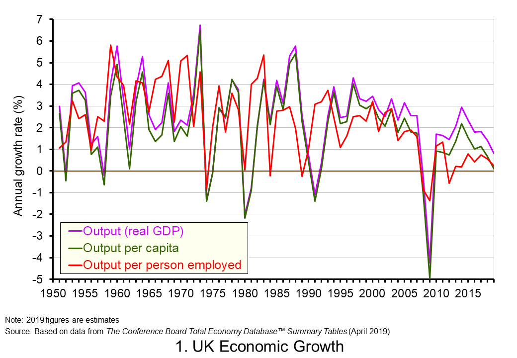 Chart 1 shows the annual rates of growth in real GDP and real GDP per capita from the 1950s. The average growth rates are 2.4 and 1.9 per cent respectively. The other series shown is the annual growth in real GDP per person employed. This is a measure of the growth in labour productivity. Its average annual growth rate is also 1.9 per cent. This illustrates the intrinsic long-run relationship between labour productivity growth and the growth rate of GDP per capita and hence in general living stanadards. (Click here to download a PowerPoint copy of the chart.)
In the short term, rates of growth in output per worker (labour productivity) and GDP per capita (general living standards) can be less similar. For example, when unemployment rates rise labour productivity rates may be little affected despite GDP per capita falling. Nonetheless, the important point here is the close long-run relationship between the growth in labour productivity and GDP per capita. This then raises an important question: what factors contribute to the growth in output and labour productivity?
An approach known as growth accounting helps to identify four key contributors to the growth of total output. The first is the quantity of labour, commonly measured in labour hours. The second is the quality of labour, also known as labour composition. Third is capital services which are physical inputs into production and include machinery, structures and IT capital. Capital services are affected by quantity and quality, but, unlike labour, it is practically more difficult to separate out these dimensions. Fourth, is Total Factor Productivity (TFP).
TFP it is essentially the residual contribution to output growth that cannot be explained by changes in the quantity and quality of the individual inputs. Hence, in principle, it is capturing changes in how effectively the labour and capital inputs are being employed and combined in production. The Conference Board’s Productivity Brief describes the growth in TFP as providing ‘a more accurate picture of the overall efficiency by which capital, labour and skills are combined in the production process’.
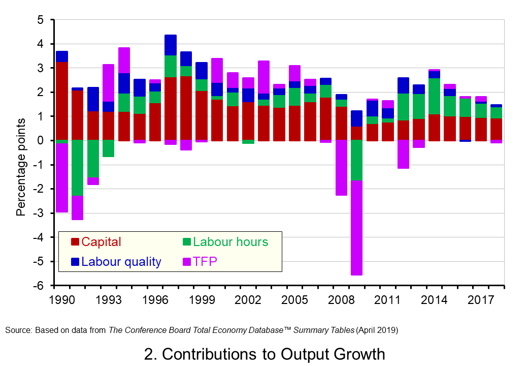 Chart 2 shows Conference Board estimates of the percentage point contribution of these four sources of growth since 1990. Over this period, output growth averaged 2 per cent per year. The contribution of capital services and, hence, what is known as capital accumulation is particularly significant at 1.5 percentage points per year. This has been significantly larger than the contribution of labour hours which averaged only 0.3 percentage points per year since 1990. This evidences the importance played by capital deepening for output growth in the UK. (Click here to download a PowerPoint copy of the chart.)
Capital deepening captures the growth in capital services relative to the growth in the labour input. It takes on even greater significance when we think about the growth in labour productivity since, after all, this is the growth in output relative to the quantity of labour. It is significant though that since 2015 the growth of capital services has contributed only 1 percentage point to output growth while the growth of labour hours has contributed an average of 0.7 percentage points. This points to a slowdown in capital deepening and hence in the growth of labour productivity.
Chart 2 also illustrates the importance of TFP growth to overall output growth. It is also important (along with capital deepening and the growth in labour quality) for the growth in labour productivity. Interestingly, we observe significant fluctuations in the growth of TFP. This is thought to reflect fluctuations in the utilisation of inputs. For example, if the utilisation of inputs falls (rises) when output falls (increases) this will be mirrored by a disproportionately large fall (increase) in TFP. In the longer-term, however, changes in TFP capture aspects of technological progress and advancement that enable more effective production methods and techniques to be deployed. In other words, the growth of TFP captures the ability of production to benefit from the advancement in ideas, products, processes and know-how.
A decline in the growth in TFP growth following the financial crisis is found quite widely in mature economies. The annual rate of growth of TFP across mature economies fell from 0.5 per cent year in 2000-2007 to 0.2 per cent in 2010-2017. In the UK this fall was from 0.5 per cent to -0.1 per cent. Hence, the decline in TFP growth of 0.6 percentage points between 2010 and 2017 was double the 0.3 percentage point fall across all mature economies. In 2018 the Conference Board estimate that TFP in the UK fell by 0.1 percent further exacerbating the downward pressure on labour productivity.
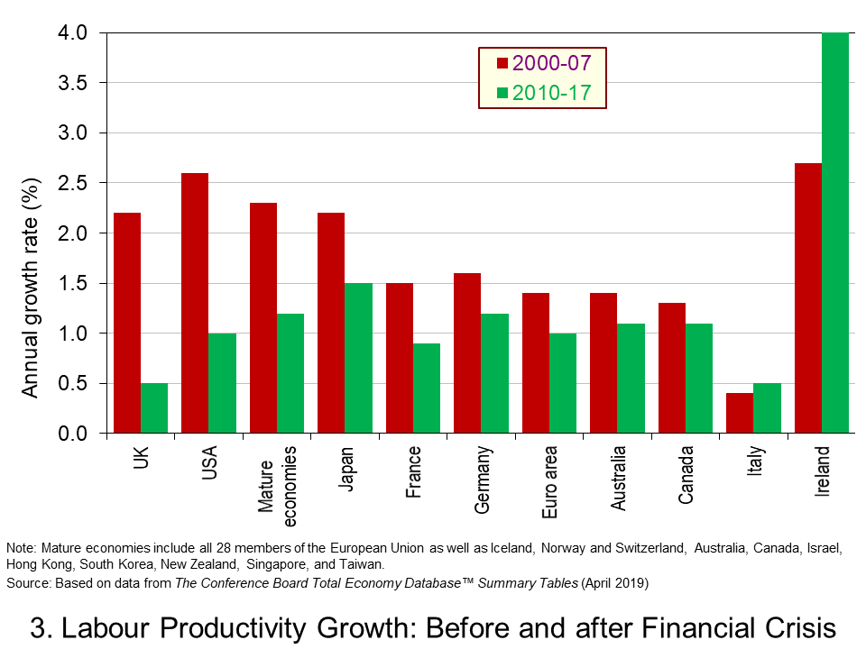 As our final chart shows, it is the magnitude to which labour productivity has eased following the financial crisis that sets the UK apart. While across all mature economies the growth of output per labour hour (another measure of labour productivity growth) fell from an average of 2.3 per cent per year in 2000-2007 to 1.2 per cent in 2010-2017, in the UK the fall was from 2.2 per cent to 0.5 per cent per year. (Click here to download a PowerPoint copy of the chart.)
While the productivity problem facing the UK is not new, the latest figures comes as a very timely reminder of the extent of the problem. To some extent the uncertainty around Brexit and the negative impact on capital accumulation has only helped to exacerbate the problem. But, this may mask a more systemic problem facing the UK. Getting to the root of this problem matters. It matters most significantly for our long-term wellbeing and prosperity. The productivity gap with our major industrial competitors is a gap that policymakers need not only to be mindful of but one that needs closing.
Articles
Questions
- What do you understand by the term labour productivity. How could we measure it?
- Why is it important to look at the growth of output per capita when assessing the benefits of long-term growth?
- Why is labour productivity important for the long-term well-being of a country?
- What do you understand by the method of growth accounting?
- What is the distinction between capital accumulation and capital deepening?
- What might explain why the growth of labour productivity has been lower in the years following the post-financial crisis?
- What do you understand by Total Factor Productivity (TFP)?
- What does the long-term growth of TFP attempt to capture?
- If you were an economic advisor to the government, what types of policy initiatives might you recommend for a government concerned about low rates of growth of labour productivity?
 The Institute of Fiscal Studies (IFS) has just published its annual ‘Green Budget‘. This is, in effect, a pre-Budget report (or a substitute for a government ‘Green Paper’) and is published ahead of the government’s actual Budget.
  But can fiscal policy be used over the longer term to offset the downward shock of Brexit, and especially a no-deal Brexit? The problem is that, if the government wishes to prevent government borrowing from soaring, it would then have to start reining in public spending again. Another period of austerity would be likely.
 With the prospects of weaker global economic growth and continuing worries about trade wars, central banks have been loosening monetary policy. The US central bank, the Federal Reserve,
  But there are two key issues with looser monetary policy.
 It’s been a while since I last blogged about labour markets and, in particular, about the effect of automation on wages and employment. My most recent post on this topic was on the 14th of April 2018 and it was mostly a reflection on some interesting findings that had been reported by Acemoglu et al (2017). More specifically, Acemoglu and Restrepo (2017) developed a theoretical framework to evaluate the effect of AI on employment and wages. They concluded that the effect was negative and potentially sizeable (for a more detailed discussion
 Donald Trump has suggested that the Fed should cut interest rates by 1 percentage point and engage in a further round of quantitative easing. He wants to see monetary policy used to give a substantial boost to US economic growth at a time when inflation is below target. In a pair of tweets just before the meeting of the Fed to decide on interest rates, he said:
 Since December 2015 the Fed has been raising interest rates by 0.25 percentage points at a time in a series of steps, so that the federal funds rate stands at between 2.25% and 2.5% (see chart). And since October 2017, it has also been engaged in
  The second issue is whether Trump’s proposed policy is a wise one.
 For these reasons, the Fed resisted calls for a large cut in interest rates and a return to quantitative easing. Instead it chose to keep interest rates on hold at its meeting on 1 May 2019.
 Chart 1 shows the annual rates of growth in real GDP and real GDP per capita from the 1950s. The average growth rates are 2.4 and 1.9 per cent respectively. The other series shown is the annual growth in real GDP per person employed. This is a measure of the growth in labour productivity. Its average annual growth rate is also 1.9 per cent. This illustrates the intrinsic long-run relationship between labour productivity growth and the growth rate of GDP per capita and hence in general living stanadards. (Click
  Chart 2 shows Conference Board estimates of the percentage point contribution of these four sources of growth since 1990. Over this period, output growth averaged 2 per cent per year. The contribution of capital services and, hence, what is known as capital accumulation is particularly significant at 1.5 percentage points per year. This has been significantly larger than the contribution of labour hours which averaged only 0.3 percentage points per year since 1990. This evidences the importance played by capital deepening for output growth in the UK. (Click
  As our final chart shows, it is the magnitude to which labour productivity has eased following the financial crisis that sets the UK apart. While across all mature economies the growth of output per labour hour (another measure of labour productivity growth) fell from an average of 2.3 per cent per year in 2000-2007 to 1.2 per cent in 2010-2017, in the UK the fall was from 2.2 per cent to 0.5 per cent per year. (Click