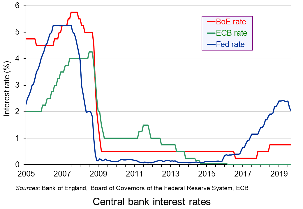
 With the prospects of weaker global economic growth and continuing worries about trade wars, central banks have been loosening monetary policy. The US central bank, the Federal Reserve, lowered its target Federal Funds rate in both July and September. Each time it reduced the rate by a quarter of a percentage point, so that it now stands at between 1.75% and 2%.
The ECB has also cut rates. In September it reduced the overnight deposit rate for banks from –0.4% to –0.5%, leaving the main rate at 0%. It also introduced a further round of quantitative easing, with asset purchases of €20 billion per month from 1 November and lasting until the ECB starts raising interest rates.
The Australian Reserve Bank has cut its ‘cash rate‘ three times this year and it now stands at an historically low level of 0.75%. Analysts are predicting that it may be forced to introduce quantitative easing if lower interest rates fail to stimulate growth.
Japan continues with its programme of quantitative easing (QE) and other central banks are considering lowering interest rates and/or (further) QE.
 But there are two key issues with looser monetary policy.
The first is whether it will be sufficient to provide the desired stimulus. With interest rates already at or near historic lows (although slightly above in the case of the USA), there is little scope for further reductions. QE may help, but without a rise in confidence, the main effect of the extra money may simply be a rise in the price of assets, such as property and shares. It may result in very little extra spending on consumption and investment – in other words, very little extra aggregate demand.
The second is the effect on inequality. By inflating asset prices, QE rewards asset owners. The wealthier people are, the more they will gain.
Many economists and commentators are thus calling for the looser monetary policy to be backed up by expansionary fiscal policy. The boost to aggregate demand, they argue, should come from higher public spending, with governments able to borrow at very low interest rates because of the loose monetary policy. Targeted spending on infrastructure would have a supply-side benefit as well as a demand-side one.
Articles
- European Central Bank cuts its deposit rate, launches new bond-buying program
CNBC, Elliot Smith (12/9/19)
- Can monetary policies help prevent a global recession?
Investment Week, Martin Gilbert (7/10/19)
- Draghi’s Utmost Is Still Not Enough
Bloomberg, John Authers (13/9/19)
- Draghi puts heat on politicians to boost fiscal stimulus with his ECB swan song
MarketWatch, William Watts (12/9/19)
- To infinity and beyond: ECB’s quantitative easing
EJ Insight, Raphael Olszyna-Marzys (2/10/19)
- The dangers of negative interest rates
Money Week, Merryn Somerset Webb (7/10/19)
- Schwarzman: Europe could enter Japan-style stagnation if governments don’t start spending
CNBC, Elliot Smith (7/10/19)
- US Fed cuts interest rates for second time since 2008
BBC News, Andrew Walker (18/9/19)
- Current Federal Reserve Interest Rates and Why They Change
The Balance, Kimberly Amadeo (19/9/19)
- Federal Reserve Interest Rate Cuts Alone Can’t Prevent a Recession
Barron’s, Al Root (4/10/19)
- Why is the Fed pumping money into the banking system?
BBC News, Natalie Sherman (19/9/19)
- Top of Lagarde’s ECB to-do list: stop QE and democratise monetary policy
Social Europe, Jens van’t Klooster (25/9/19)
- Economists warn Reserve Bank could be forced to print money if rate cuts fail to deliver
The Guardian, Martin Farrer (2/10/19)
- A very large gamble: evidence on Quantitative Easing in the US and UK
Institute for Policy Research. Policy Brief, Chris Martin and Costas Milas
- The verdict on 10 years of quantitative easing
The Guardian, Richard Partington (8/3/19)
ECB Press Conference
Questions
- Explain what is meant by quantitative easing.
- What determines the effectiveness of quantitative easing?
- Why is President Trump keen for the Federal Reserve to pursue more aggressive interest rate cuts?
- What is the Bank of England’s current attitude towards changing interest rates and/or further quantitative easing?
- What are the current advantages and disadvantages of governments pursuing a more expansionary fiscal policy?
- Compare the relative merits of quantitative easing through asset purchases and the use of ‘helicopter money’.
 There have been many analyses of the economic effects of Brexit, both before the referendum and at various times since, including analyses of the effects of the deal negotiated by Theresa May’s government and the EU. But with the prospect of a no-deal Brexit on 31 October under the new Boris Johnson government, attention has turned to the effects of leaving the EU without a deal.
There have been two major analyses recently of the likely effects of a no-deal Brexit – one by the International Monetary Fund (IMF) and one by the Office for Budget Responsibility (OBR).
IMF analysis
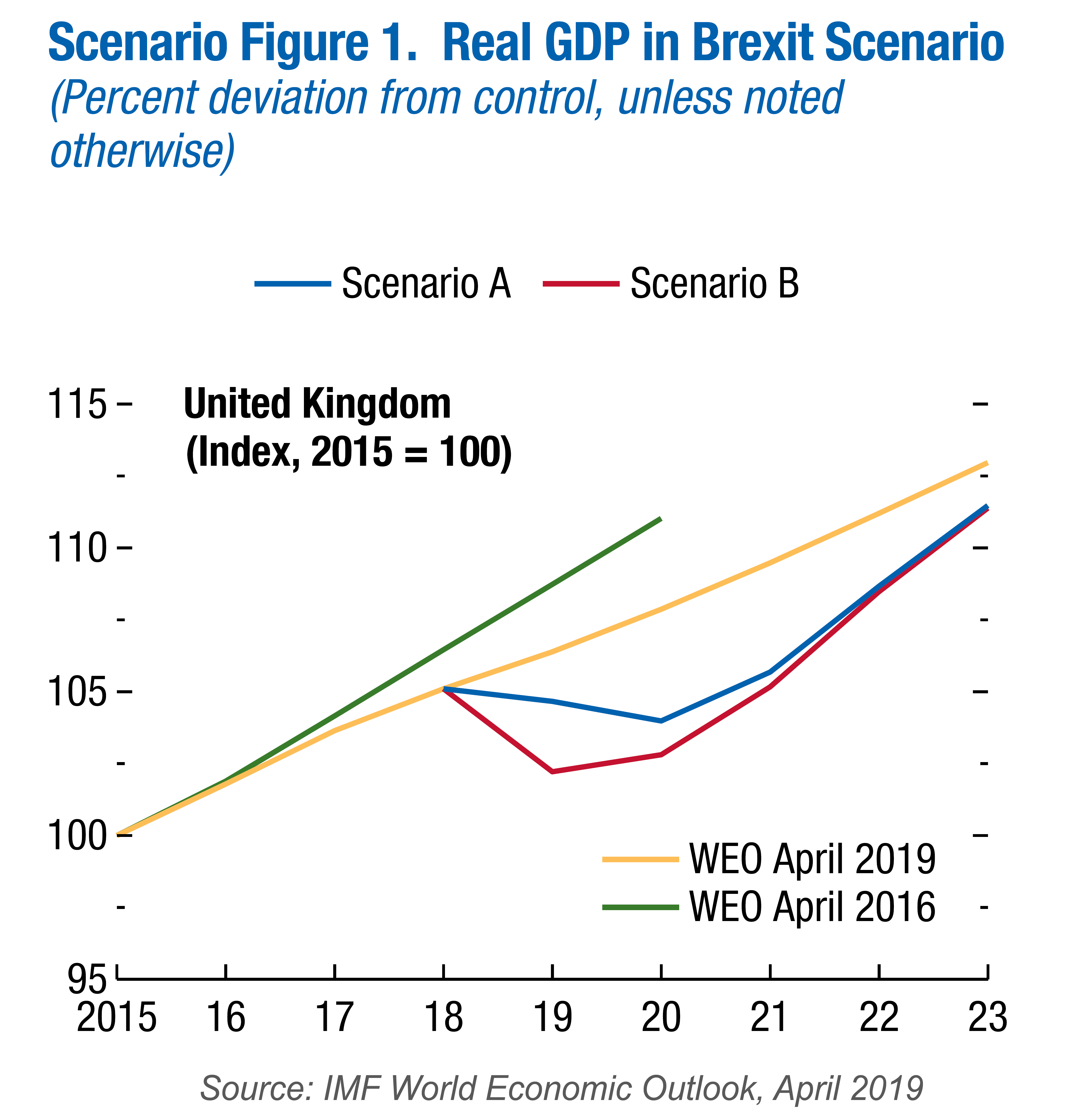
The first was in April by the IMF as part of its 6-monthly World Economic Outlook. In Scenario Box 1.1. ‘A No-Deal Brexit’ on page 28 of Chapter 1, the IMF looked at two possible scenarios.
Scenario A assumes no border disruptions and a relatively small increase in UK sovereign and corporate spreads. Scenario B incorporates significant border disruptions that increase import costs for UK firms and households (and to a lesser extent for the European Union) and a more severe tightening in financial conditions.
 Under both scenarios, UK exports to the EU and UK imports from the EU revert to WTO rules. As a result, tariffs are imposed by mid-2020 or earlier. Non-tariff barriers rise at first but are gradually reduced over time. Most free-trade arrangements between the EU and other countries are initially unavailable to the UK (see the blog EU strikes major trade deals) but both scenarios assume that ‘new trade agreements are secured after two years, and on terms similar to those currently in place.’
Both scenarios also assume a reduction in net immigration from the EU of 25 000 per year until 2030. Both assume a rise in corporate and government bond rates, reflecting greater uncertainty, with the effect being greater in Scenario B. Both assume a relaxing of monetary and fiscal policy in response to downward pressures on the economy.
The IMF analysis shows a negative impact on UK GDP, with the economy falling into recession in late 2019 and in 2020. This is the result of higher trade costs and reduced business investment caused by a poorer economic outlook and increased uncertainty. By 2021, even under Scenario A, GDP is approximately 3.5% lower than it would have been if the UK had left the EU with the negotiated deal. For the rest of the EU, GDP is around 0.5% lower, although the effect varies considerably from country to country.
The IMF analysis makes optimistic assumptions, such as the UK being able to negotiate new trade deals with non-EU countries to replace those lost by leaving. More pessimistic assumptions would lead to greater costs.
OBR analysis
Building on the analysis of the IMF, the Office for Budget Responsibility considered the effect of a no-deal Brexit on the public finances in its biennial Fiscal risks report, published on 17 July 2019. This argues that, under the relatively benign Scenario A assumptions of the IMF, the lower GDP would result in annual public-sector net borrowing (PSNB) rising. By 2021/22, if the UK had left with the deal negotiated with the EU, PSNB would have been around £18bn. A no-deal Brexit would push this up to around £51bn.
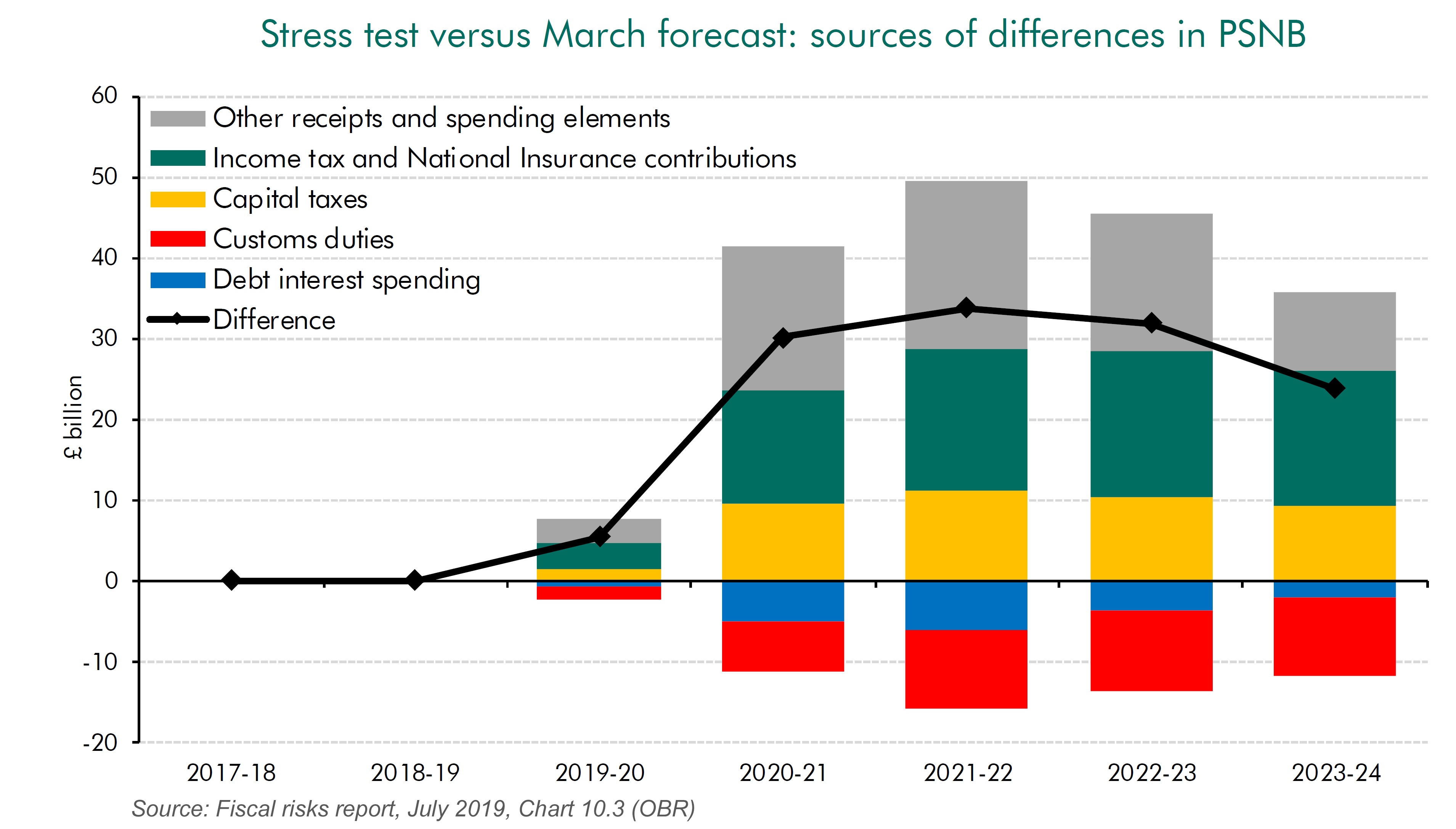
According to the OBR, the contributors to this rise in public-sector net borrowing of around £33bn are:
- A fall in income tax and national insurance receipts of around £16.5bn per year because of lower incomes.
- A fall in corporation tax and expenditure taxes, such as VAT, excise duties and stamp duty of around £22.5bn per year because of lower expenditure.
- A fall in capital taxes, such as inheritance tax and capital gains tax of around £10bn per year because of a fall in asset prices.
- These are offset to a small degree by a rise in customs duties (around £10bn) because of the imposition of tariffs and by lower debt repayments (of around £6bn) because of the Bank of England having to reduce interest rates.
The rise in PSNB would constrain the government’s ability to use fiscal policy to boost the economy and to engage in the large-scale capital projects advocated by Boris Johnson while making the substantial tax cuts he is proposing. A less optimistic set of assumptions would, of course, lead to a bigger rise in PSNB, which would further constrain fiscal policy.
Articles
Video
Reports
Questions
- What are the assumptions of the IMF World Economic Outlook forecasts for the effects of a no-deal Brexit? Do you agree with these assumptions? Explain.
- What are the assumptions of the analysis of a no-deal Brexit on the public finances in the OBR’s Fiscal risks report? Do you agree with these assumptions? Explain.
- What is the difference between forecasts and analyses of outcomes?
- For what reasons might growth over the next few years be higher than in the IMF forecasts under either scenario?
- For what reasons might growth over the next few years be lower than in the IMF forecasts under either scenario?
- For what reasons might public-sector net borrowing (PSNB) over the next few years be lower than in the OBR forecast?
- For what reasons might PSNB over the next few years be higher than in the OBR forecast?
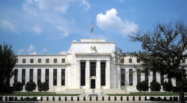 Donald Trump has suggested that the Fed should cut interest rates by 1 percentage point and engage in a further round of quantitative easing. He wants to see monetary policy used to give a substantial boost to US economic growth at a time when inflation is below target. In a pair of tweets just before the meeting of the Fed to decide on interest rates, he said:
China is adding great stimulus to its economy while at the same time keeping interest rates low. Our Federal Reserve has incessantly lifted interest rates, even though inflation is very low, and instituted a very big dose of quantitative tightening. We have the potential to go up like a rocket if we did some lowering of rates, like one point, and some quantitative easing. Yes, we are doing very well at 3.2% GDP, but with our wonderfully low inflation, we could be setting major records &, at the same time, make our National Debt start to look small!
But would this be an appropriate policy? The first issue concerns the independence of the Fed.
It is supposed to take decisions removed from the political arena. This means sticking to its inflation target of 2 per cent over the medium term – the target it has officially had since January 2012. To do this, it adjusts the federal funds interest rate and the magnitude of any bond buying programme (quantitative easing) or bond selling programme (quantitative tightening).
The Fed is supposed to assess the evidence concerning the pressures on inflation (e.g. changes in aggregate demand) and what inflation is likely to be over the medium term in the absence of any changes in monetary policy. If the Federal Open Market Committee (FOMC) expects inflation to exceed 2 per cent over the medium term, it will probably raise the federal funds rate; if it expects inflation to be below the target it will probably lower the federal funds rate.
In the case of the economy being in recession, and thus probably considerably undershooting the target, it may also engage in quantitative easing (QE). If the economy is growing strongly, it may sell some of its portfolio of bonds and thus engage in quantitative tightening (QT).
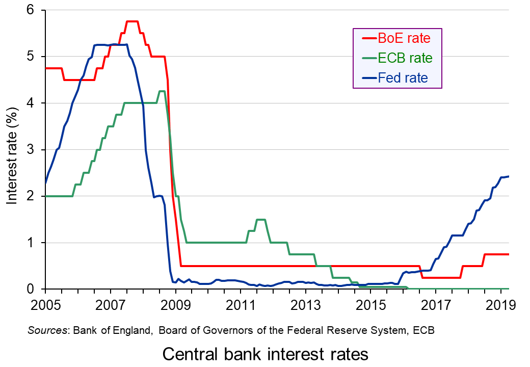 Since December 2015 the Fed has been raising interest rates by 0.25 percentage points at a time in a series of steps, so that the federal funds rate stands at between 2.25% and 2.5% (see chart). And since October 2017, it has also been engaged in quantitative tightening. In recent months it has been selling up to $50 billion of assets per month from its holdings of around $4000 billion and so far has reduced them by around £500 billion. It has, however, announced that the programme of QT will end in the second half of 2019.
This does raise the question of whether the FOMC is succumbing to political pressure to cease QT and put interest rate rises on hold. If so, it is going against its remit to base its policy purely on evidence. The Fed, however, maintains that its caution reflects uncertainty about the global economy.
 The second issue is whether Trump’s proposed policy is a wise one.
Caution about further rises in interest rates and further QT is very different from the strongly expansionary monetary policy that President Trump proposes. The economy is already growing at 3.2%, which is above the rate of growth in potential output, of around 1.8% to 2.0%. The output gap (the percentage amount that actual GDP exceeds potential GDP) is positive. The IMF forecasts that the gap will be 1.4% in 2019 and 1.3% in 2020 and 2021. This means that the economy is operating at above normal capacity working and this will eventually start to drive up inflation. Any further stimulus will exacerbate the problem of excess demand. And a large stimulus, as proposed by Donald Trump, will cause serious overheating in the medium term, even if it does stimulate growth in the short term.
 For these reasons, the Fed resisted calls for a large cut in interest rates and a return to quantitative easing. Instead it chose to keep interest rates on hold at its meeting on 1 May 2019.
But if the Fed had done as Donald Trump would have liked, the economy would probably be growing very strongly at the time of the next US election in November next year. It would be a good example of the start of a political business cycle – something that is rarer nowadays with the independence of central banks.
Articles
FOMC meeting
Questions
- What are the arguments for central bank independence?
- Are there any arguments against central bank independence?
- Explain what is meant by an ‘output gap’? Why is it important to be clear on what is meant by ‘potential output’?
- Would there be any supply-side effects of a strong monetary stimulus to the US economy at the current time? If so, what are they?
- Explain what is meant by the ‘political business’ cycle? Are governments in the UK, USA or the eurozone using macroeconomic policy to take advantage of the electoral cycle?
- The Fed seems to be ending its programme of quantitative tightening (QT). Why might that be so and is it a good idea?
- If inflation is caused by cost-push pressures, should central banks stick rigidly to inflation targets? Explain.
- How are expectations likely to affect the success of a monetary stimulus?
 Consumer credit is borrowing by individuals to finance current expenditure on goods and services. Consumer credit is distinct from lending secured on dwellings (referred to more simply as ‘secured lending’). Consumer credit comprises lending on credit cards, lending through overdraft facilities and other loans and advances, for example those financing the purchase of cars. We consider here recent trends in the flows of consumer credit in the UK and discuss their implications.
Analysing consumer credit data is important because the growth of consumer credit has implications for the financial wellbeing or financial health of individuals and, of course, for financial institutions. As we shall see shortly, the data on consumer credit is consistent with the existence of credit cycles. Cycles in consumer credit have the potential to be not only financially harmful but economically destabilising. After all, consumer credit is lending to finance spending and therefore the amount of lending can have significant effects on aggregate demand and economic activity.
Data on consumer credit are available monthly and so provide an early indication of movements in economic activity. Furthermore, because lending flows are likely to be sensitive to changes in the confidence of both borrowers and lenders, changes in the growth of consumer credit can indicate turning points in the economy and, hence, in the macroeconomic environment.
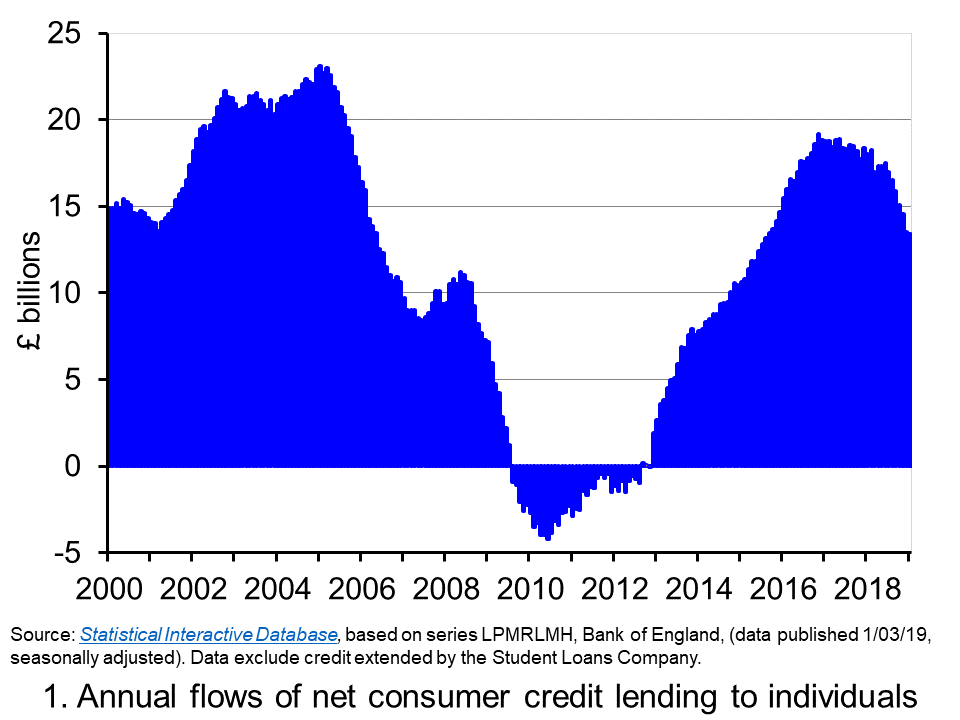 Chart 1 shows the annual flows of net consumer credit since 2000 – the figures are in £ billions. Net flows are gross flows less repayments. (Click here to download a PowerPoint copy of the chart.) In January 2005 the annual flow of net consumer credit peaked at £23 billion, the equivalent of just over 2.5 per cent of annual disposable income. This helped to fuel spending and by the final quarter of the year, the economy’s annual growth rate had reached 4.8 per cent, significantly about its long-run average of 2.5 per cent.
By 2009 net consumer credit flows had become negative. This meant that repayments were greater than additional flows of credit. It was not until 2012 that the annual flow of net consumer credit was again positive. Yet by November 2016, the annual flow of net consumer credit had rebounded to over £19 billion, the equivalent of just shy of 1.5 per cent of annual disposable income. This was the largest annual flow of consumer credit since September 2005.
Although the strength of consumer credit in 2016 was providing the economy with a timely boost to growth in the immediate aftermath of the referendum on the UK’s membership of the EU, it nonetheless raised concerns about its sustainability. Specifically, given the short amount of time that had elapsed since the financial crisis and the extreme levels of financial distress that had been experienced by many sectors of the economy, how susceptible would people and organisations be to a future economic slowdown and/or rise in interest rates?
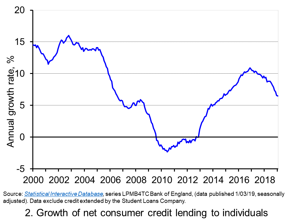 The extent to which the economy experiences consumer credit cycles can be seen even more readily by looking at the 12-month growth rate in the net consumer credit. In essence, this mirrors the growth rate in the stock of consumer credit. Chart 2 evidences the double-digit growth rates in net consumer credit lending experienced during the first half of the 2000s. Growth rates then eased but, as the financial crisis unfolded, they plunged sharply. (Click here to download a PowerPoint copy of the chart.)
Yet, as Chart 2 shows, consumer credit growth began to recover quickly from 2013 so that by 2016 the annual growth rate of net consumer credit was again in double figures. In November 2016 the 12-month growth rate of net consumer credit peaked at 10.9 per cent. Thereafter, the growth rate has continually eased. In January 2019 the annual growth rate of net consumer credit had fallen back to 6.5 per cent, the lowest rate since October 2014.
The easing of consumer credit is likely to have been influenced, in part, by the resumption in the growth of real earnings from 2018 (see Getting real with pay). Yet, it is hard to look past the economic uncertainties around Brexit.
Uncertainty tends to cause people to be more cautious. With the heightened uncertainty that has has characterised recent times, it is likely that for many people and businesses prudence has dominated impatience. Therefore, in summary, it appears that prudence is helping to steer borrowing along a downswing in the credit cycle. As it does, it helps to put a further brake on spending and economic growth.
Articles
Questions
- What is the difference between gross and net lending?
- Consider the argument that we should be worried more by excessive growth in consumer credit than on lending secured on dwellings?
- How could we measure whether different sectors of the economy had become financially distressed?
- What might explain why an economy experiences credit cycles?
- Explain how the growth in net consumer credit can affect economic activity?
- If people are consumption smoothers, how can credit cycles arise?
- What are the potential policy implications of credit cycles?
- It is said that when making financial decisions people face an inter-temporal choice. Explain what you understand this by this concept.
- If economic uncertainty is perceived to have increased how could this affect the consumption, saving and borrowing decisions of people?
 Growth in the eurozone has slowed. The European Central Bank (ECB) now expects it to be 1.1% this year; in December, it had forecast a rate of 1.7% for 2019. Mario Draghi, president of the ECB, in his press conference, said that ‘the weakening in economic data points to a sizeable moderation in the pace of the economic expansion that will extend into the current year’. Faced with a slowing eurozone economy, the ECB has announced further measures to stimulate economic growth.
First it has indicated that interest rates will not rise until next year at the earliest ‘and in any case for as long as necessary to ensure the continued sustained convergence of inflation to levels that are below, but close to, 2% over the medium term’. The ECB currently expects HIPC inflation to be 1.2% in 2019. It was expected to raise interest rates later this year – probably by the end of the summer. The ECB’s main refinancing interest rate, at which it provides liquidity to banks, has been zero since March 2016, and so there was no scope for lowering it.
 Second, although quantitative easing (the asset purchase programme) is coming to an end, there will be no ‘quantitative tightening’. Instead, the ECB will purchase additional assets to replace any assets that mature, thereby leaving the stock of assets held the same. This would continue ‘for an extended period of time past the date when we start raising the key ECB interest rates, and in any case for as long as necessary to maintain favourable liquidity conditions and an ample degree of monetary accommodation’.
Third, the ECB is launching a new series of ‘quarterly targeted longer-term refinancing operations (TLTRO-III), starting in September 2019 and ending in March 2021, each with a maturity of two years’. These are low-interest loans to banks in the eurozone for use for specific lending to businesses and households (other than for mortgages) at below-market rates. Banks will be able to borrow up to 30% of their eligible assets (yet to be fully defined). These, as their acronym suggests, are the third round of such loans. The second round was relatively successful. As the Barron’s article linked below states:
Banks boosted their long-term borrowing from the ECB by 70% over the course of the program, although they did not manage to increase their holdings of business loans until after TLTRO II had finished disbursing funds in March 2017.
Whether these measures will be enough to raise growth rates in the eurozone depends on a range of external factors affecting aggregate demand. Draghi identified three factors which could have a negative effect.
- Brexit. The forecasts assume an orderly Brexit in accordance with the withdrawal deal agreed between the European Commission and the UK government. With the House of Commons having rejected this deal twice, even though it has agreed that there should not be a ‘no-deal Brexit’, this might happen as it is the legal default position. This could have a negative effect on the eurozone economy (as well as a significant one on the UK economy). Even an extension of Article 50 could create uncertainty, which would also have a negative effect
- Trade wars. If President Trump persists with his protectionist policy, this will have a negative effect on growth in the eurozone and elsewhere.
- China. Chinese growth has slowed and this dampens global growth. What is more, China is a major trading partner of the eurozone countries and hence slowing Chinese growth impacts on the eurozone through the international trade multiplier. The ECB has taken this into account, but if Chinese growth slows more than anticipated, this will further push down eurozone growth.
Then there are internal uncertainties in the eurozone, such as the political and economic uncertainty in Italy, which in December 2018 entered a recession (2 quarters of negative economic growth). Its budget deficit is rising and this is creating conflict with the European Commission. Also, there are likely to be growing tensions within Italy as the government raises taxes.
Faced with these and other uncertainties, the measures announced by Mario Draghi may turn out not to be enough. Perhaps in a few months’ there may have to be a further round of quantitative easing.
Articles
- ECB statement following policy meeting
Reuters, Larry King (7/3/19)
- European Central Bank acts to boost struggling eurozone
BBC News, Andrew Walker (7/3/19)
- The European Central Bank Tries to Avoid Repeating Past Mistakes
Barron’s, Matthew C. Klein (8/3/19)
- ECB pushes back rate hike plans, announces fresh funding for banks
CNBC, Silvia Amaro (7/3/19)
- Why the ECB Followed the Fed’s Flip-Flopping
Bloomberg, Mohamed A. El-Erian (7/3/19)
- Central Banks Don’t Have the Answer and Markets Know It
Bloomberg, Robert Burgess (7/3/19)
- Missing out on monetary normalisation
OMFIF, David Marsh (12/4/19)
- The ECB is attempting to get ahead of event
Financial Times, The editorial board (8/3/19)
- Explainer: What is the fuss about European Central Bank TLTRO loans?
Reuters, Balazs Koranyi (4/3/19)
Videos
ECB publications
Questions
- Investigate the history of quantitative easing and its use by the Fed, the Bank of England and the ECB. What is the current position of the three central banks on ‘quantitative tightening’, whereby central banks sell some of the stock of assets they have purchased during the process of quantitative easing or not replace them when they mature?
- What are TLTROs and what use of them has been made by the ECB? Do they involve the creation of new money?
- What will determine the success of the proposed TLTRO III scheme?
- If the remit of central banks is to keep inflation on target, which in the ECB’s case means below 2% HIPC inflation but close to it over the medium term, why do people talk about central banks using monetary policy to revive a flagging economy?
- What is ‘forward guidance’ by central banks and what determines its affect on aggregate demand?
 With the prospects of weaker global economic growth and continuing worries about trade wars, central banks have been loosening monetary policy. The US central bank, the Federal Reserve, lowered its target Federal Funds rate in both July and September. Each time it reduced the rate by a quarter of a percentage point, so that it now stands at between 1.75% and 2%.
 But there are two key issues with looser monetary policy.
  ECB Press Conference
 There have been many analyses of the
  Under both scenarios, UK exports to the EU and UK imports from the EU revert to WTO rules. As a result, tariffs are imposed by mid-2020 or earlier. Non-tariff barriers rise at first but are gradually reduced over time. Most free-trade arrangements between the EU and other countries are initially unavailable to the UK (see the blog
 Donald Trump has suggested that the Fed should cut interest rates by 1 percentage point and engage in a further round of quantitative easing. He wants to see monetary policy used to give a substantial boost to US economic growth at a time when inflation is below target. In a pair of tweets just before the meeting of the Fed to decide on interest rates, he said:
 Since December 2015 the Fed has been raising interest rates by 0.25 percentage points at a time in a series of steps, so that the federal funds rate stands at between 2.25% and 2.5% (see chart). And since October 2017, it has also been engaged in
  The second issue is whether Trump’s proposed policy is a wise one.
 For these reasons, the Fed resisted calls for a large cut in interest rates and a return to quantitative easing. Instead it chose to keep interest rates on hold at its meeting on 1 May 2019.
 Consumer credit is borrowing by individuals to finance current expenditure on goods and services. Consumer credit is distinct from lending secured on dwellings (referred to more simply as ‘secured lending’). Consumer credit comprises lending on credit cards, lending through overdraft facilities and other loans and advances, for example those financing the purchase of cars. We consider here recent trends in the flows of consumer credit in the UK and discuss their implications.
 Chart 1 shows the annual flows of net consumer credit since 2000 – the figures are in £ billions. Net flows are gross flows less repayments. (Click
  The extent to which the economy experiences consumer credit cycles can be seen even more readily by looking at the 12-month growth rate in the net consumer credit. In essence, this mirrors the growth rate in the stock of consumer credit. Chart 2 evidences the double-digit growth rates in net consumer credit lending experienced during the first half of the 2000s. Growth rates then eased but, as the financial crisis unfolded, they plunged sharply. (Click
  Growth in the eurozone has slowed. The European Central Bank (ECB) now expects it to be 1.1% this year; in December, it had forecast a rate of 1.7% for 2019. Mario Draghi, president of the ECB, in his
  Second, although quantitative easing (the asset purchase programme) is coming to an end, there will be no ‘quantitative tightening’. Instead, the ECB will purchase additional assets to replace any assets that mature, thereby leaving the stock of assets held the same. This would continue ‘for an extended period of time past the date when we start raising the key ECB interest rates, and in any case for as long as necessary to maintain favourable liquidity conditions and an ample degree of monetary accommodation’.