 In the second of a series of blogs looking at applications of the distinction between nominal and real indicators, we revisit the blog Getting Real with Growth last updated in October 2021.
In this blog, we discuss how, in making a meaningful comparison over time of a country’s national income and, therefore, the aggregate purchasing power of its people, we need to take inflation into account. Likewise, if we want to analyse changes in the volume of production, we need to eliminate the effects of price changes on GDP. This is important when analysing the business cycle and identifying periods of boom or bust. Hence, in this updated blog we take another look at what real GDP data reveal about both longer-term economic growth and the extent of economic volatility – or what we refer to as the twin characteristics of economic growth.
Real and nominal GDP
The nominal (or current-price) estimate for UK gross domestic product in 2023 was £2.687 trillion. The estimate of national output or national income is based primarily on the production of final goods and services and, hence, purchased by the final user. It therefore largely excludes intermediate goods and services: i.e. goods and services that are transformed or used up in the process of making something else, although data on imports and exports do include intermediate goods and services. The 2023 figure represents a nominal increase in national income of 7.2 per cent on the £2.51 trillion recorded in 2022. These values make no adjustment for inflation and therefore reflect the prices of output that were prevailing at the time.
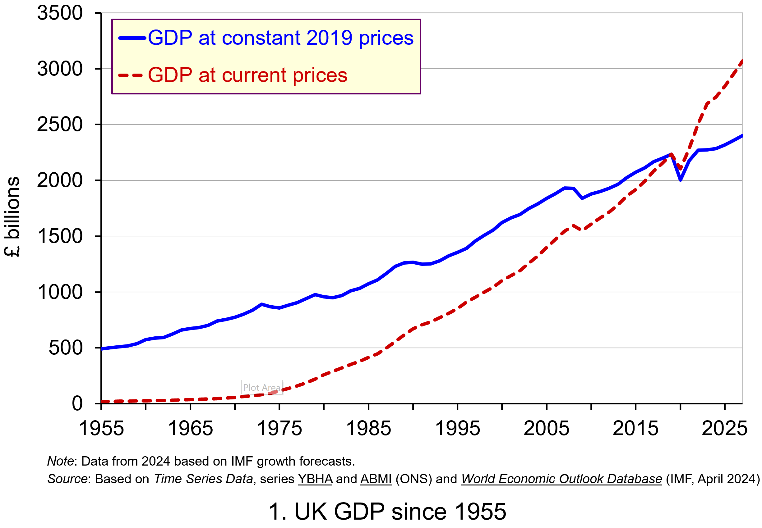 Chart 1 shows current-price estimates of GDP from 1955, when the value of GDP was estimated at £19.2 billion. The £2.687 trillion figure recorded for 2023 is an increase of over 140 times that in 1955, a figure that rises to 160 times if we compare the 1950 value with the latest IMF estimate for 2027. However, if we want to make a more meaningful comparison of the country’s national income we need to adjust for inflation. (Click here to download a PowerPoint of the chart.)
Long-term growth in real GDP
If we measure GDP at constant prices, we eliminate the effect of inflation. To construct a constant-price series for GDP, a process known as chain-linking is used. This involves taking consecutive pairs of years, e.g. 2022 and 2023, and estimating what GDP would be in the most recent year (in this case, 2023) if the previous year’s prices (i.e. 2022) had continued to prevail. By calculating the percentage change from the previous year’s GDP value we have an estimate of the volume change. If this is repeated for other pairs of years, we have a series of percentage changes that capture the volume changes from year-to-year. Finally, a reference year is chosen and the percentage volume changes are applied backwards and forwards from the nominal GDP value for the reference year.
In effect, a real GDP series creates a quantity measure in monetary terms. Chart 1 shows GDP at constant 2019 prices (real GDP) alongside GDP at current prices (nominal GDP). Consider first the real GDP numbers for 1955 and 2023. GDP in 1950 at 2019 prices was £491.2 billion. This is higher than the current-price value because prices in 2019 (the reference year) were higher than those in 1955. Meanwhile, GDP in 2023 when measured at 2019 prices was £2.273 trillion. This constant-price value is smaller than the corresponding current-price value because prices in 2019 where lower than those in 2023.
 Between 1955 and 2023 real GDP increased 4.6 times. If we extend the period to 2027, again using the latest IMF estimates, the increase is 4.9 times. Because we have removed the effect of inflation, the real growth figure is much lower than the nominal growth figure.
Crucially, what we are left with is an indicator of the long-term growth in the volume of the economy’s output and hence an increase in national income that is backed up by an increase in production. Whereas nominal growth rates are affected by changes in both volumes and prices, real growth rates reflect only changes in volumes.
The upward trajectory observed in constant-price GDP is therefore evidence of positive longer-term growth. This is one of the twin characteristics of growth.
Short-term fluctuations in the growth of real GDP
The second characteristic is fluctuations in the rate of growth from period to period. We can see this second characteristic more clearly by plotting the percentage change in real GDP from year to year.
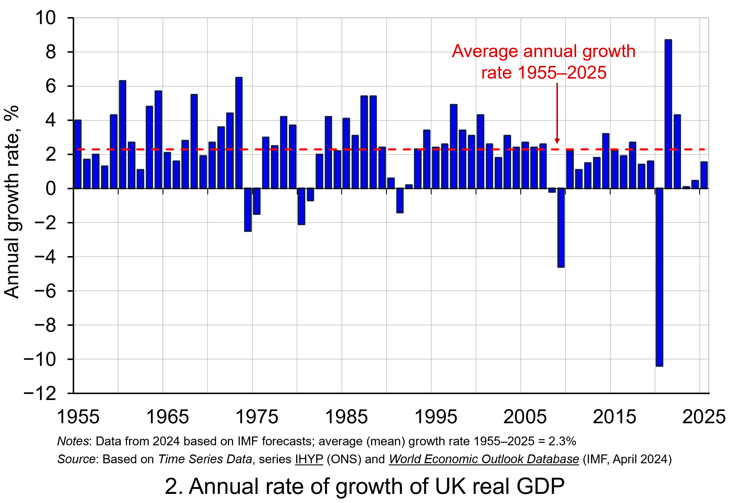 Chart 2 shows the annual rate of growth in real GDP each year from 1955 to 2025. From it, we see the inherent instability that is a key characteristic of the macroeconomic environment. This instability is, of course, mirrored in the output path of real GDP in Chart 1, but the annual rates of growth show the instability more clearly. We can readily see the impact on national output of the global financial crisis of 2007–8 and the global COVID pandemic.
In 2009, constant-price GDP in the UK fell by 4.6 per cent, whereas current-price GDP fell by 2.8 per cent. Then, in 2020, constant-price GDP and, hence, the volume of national output fell by 10.4 per cent, as compared to a 5.8 per cent fall in current-price GDP. These global, ‘once-in-a-generation’ shocks are stark examples of the instability that characterises economies and which generate the ‘ups and downs’ in an economy’s output path, known more simply as ‘the business cycle’. (Click here to download a PowerPoint copy of the chart.)
Determinants of long-and short-term growth
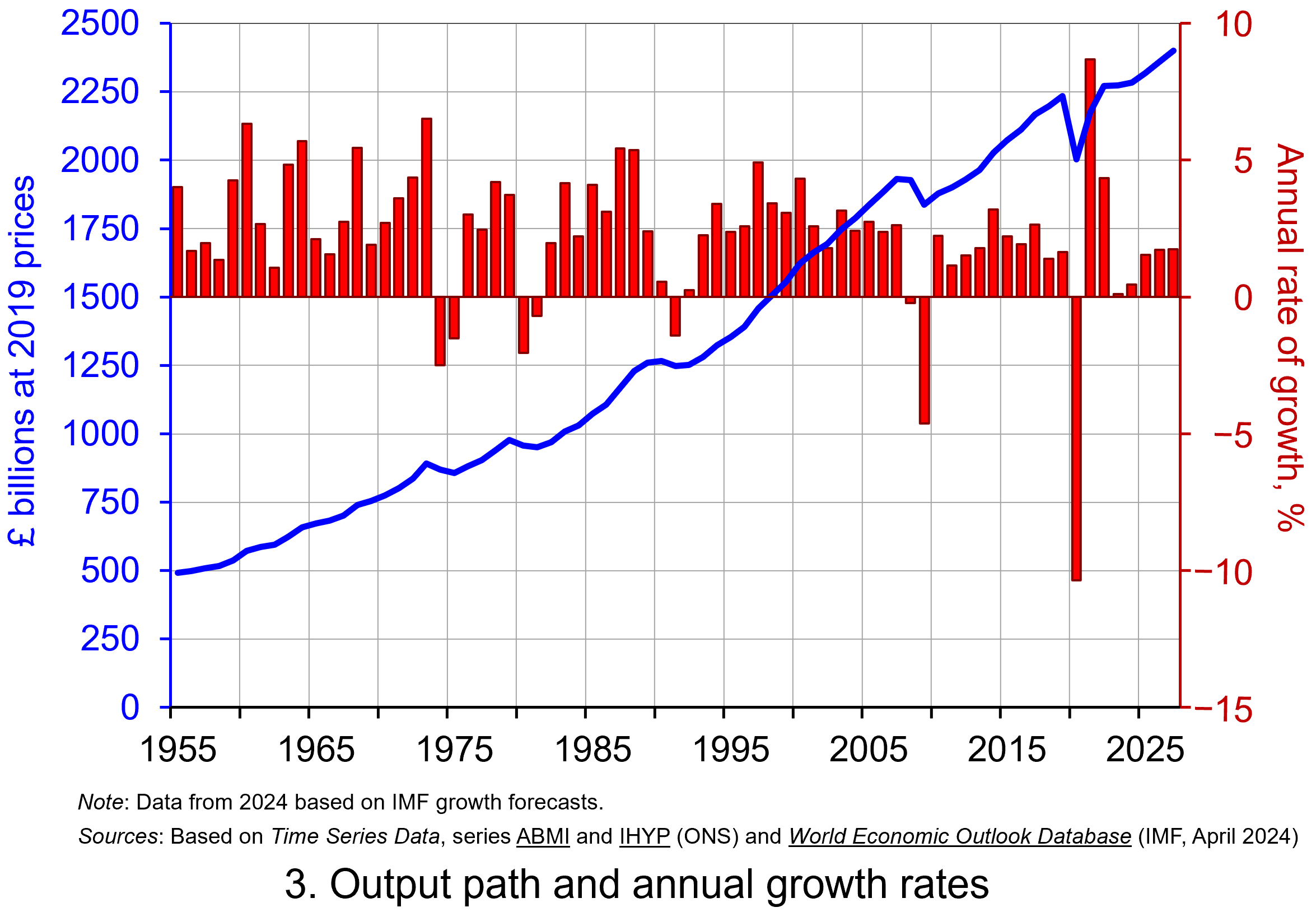 The twin characteristics of growth can be seen simultaneously by combining the output path (shown by the levels of real GDP) with the annual rates of growth. This is shown in Chart 3. The longer-term growth seen in the economy’s output path is generally argued to be driven by the quantity and quality of the economy’s resources, and their effectiveness when combined in production (i.e. their productivity). In other words, it is the supply side of the economy that determines the trajectory of the output path over the longer term. (Click here to download a PowerPoint copy of the chart.)
However, the fluctuations we observe in short-term growth rates tend to reflect shocks, also known as impulses, that originate either from the ability and or willingness of purchasers to consume (demand-side shocks) or producers to supply (supply-side shocks). These impulses are then amplified (or ‘propagated’) via the multiplier, expectations and other factors, and their effects, therefore, transmitted through the economy. Unusually in the case of the pandemic, the lockdown measures employed by governments around the world resulted in simultaneous negative aggregate demand and aggregate supply shocks.
Persistence effects
Explanations of the business cycle and of long-term growth are not mutually exclusive. The shocks and the propagation mechanisms that help to create and shape the business cycle can themselves have enduring or persistent effects on output. The global financial crisis, fuelled by unsustainable lending and the overstretch of private-sector balance sheets, which then spilt over to the public sector as governments attempted to stabilise the financial system and support aggregate demand, is argued by some to have created the conditions for low-growth persistence seen in many countries in the 2010s. This type of persistence is known as hysteresis as it originates from a negative demand shock.
Economists and policymakers were similarly concerned that the pandemic would also generate persistence in the form of scarring effects that might again affect the economy’s output path. Such concerns help to explain why many governments introduced furlough schemes to protect jobs and employment income, as well as provide grants or loans to business.
Per capita output
To finish, it is important to recognise that, when thinking about living standards, it is the growth in real GDP per capita that we need to consider. A rise in real GDP will only lead to a rise in overall living standards if it is faster than the rise in population.
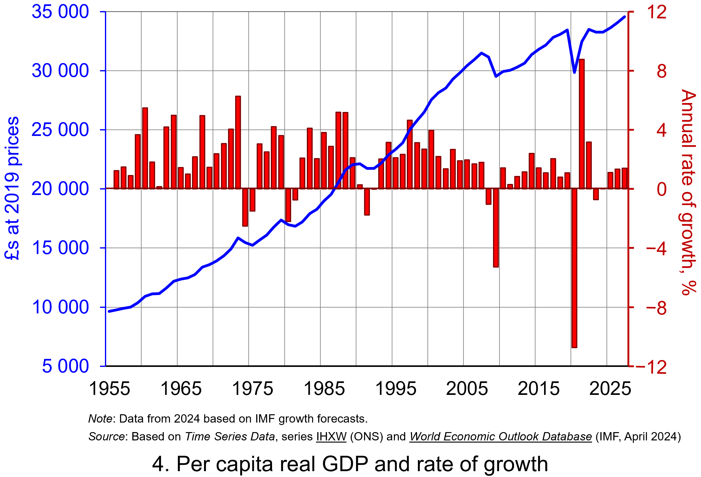 Our final chart therefore replicates Chart 3 but for real GDP per capita. Between 1955 and 2023 real GDP per capita grew by a factor of 3.45, which increases to 3.6 when we consider the period up to 2027. The average rate of growth of real GDP per capita up to 2023 was 1.87 per cent (lower than the 2.34 per cent increase in real GDP).
But the rate of increase in real GDP per capita was much higher before 2007 than it has been since. If we look at the period up to 2007 and, hence, before the global financial crisis, the figure is 2.32 per cent (2.7 per cent for real GDP), whereas from 2008 to 2023 the average rate of growth of real GDP per capita was a mere 0.42 per cent (1.1 per cent for real GDP). (Click here to download a PowerPoint copy of the chart.)
The final chart therefore reiterates the messages from recent blogs, such as Getting Real with Pay and The Productivity Puzzle, that long-term economic growth and the growth of real wages have slowed dramatically since the financial crisis. This has had important implications for the wellbeing of all sectors of the economy. The stagnation of living standards is therefore one of the most important economic issues of our time. It is one that the incoming Labour government will be keen to address.
Data and Reports
- Steady but slow: Resilience amid divergence
- IMF World Economic Outlook Database
- Gross Domestic Product
World Economic Outlook April 2024
IMF
ONS time series data and publications
Articles
- UK economy grew more than estimated in early 2024
- UK service sector growth ‘seizes up’ as firms put plans on hold before election
- Low investment blocking UK growth, says think tank
- What is GDP, how is it measured and why does it matter?
- Five key asks for new UK Government to boost economic growth
BBC News, Michael Race (28/6/24)
The Guardian, Richard Partington (3/7/24)
BBC News, Nick Edser and Charlotte Edwards (18/6/24)
BBC News (28/6/24)
The Herald, Stuart Patrick (4/7/24)
Questions
- What do you understand by the term ‘macroeconomic environment’? What data could be used to describe the macroeconomic environment?
- When a country experiences positive rates of inflation, which is higher: nominal economic growth or real economic growth?
- Does an increase in nominal GDP mean a country’s production has increased? Explain your answer.
- Does a decrease in nominal GDP mean a country’s production has decreased? Explain your answer.
- Why does a change in the growth of real GDP allow us to focus on what has happened to the volume of production?
- What does the concept of the ‘business cycle’ have to do with real rates of economic growth?
- When would falls in real GDP be classified as a recession?
- Distinguish between the concepts of ‘short-term growth’ and ‘longer-term growth’.
- What do you understand by the term ‘persistence’ in macroeconomics? Given examples of persistence effects and the means by which they can be generated?
- Discuss the proposition that the pandemic could have a positive effect on longer-term growth rates because of the ways that people and business have had to adapt.
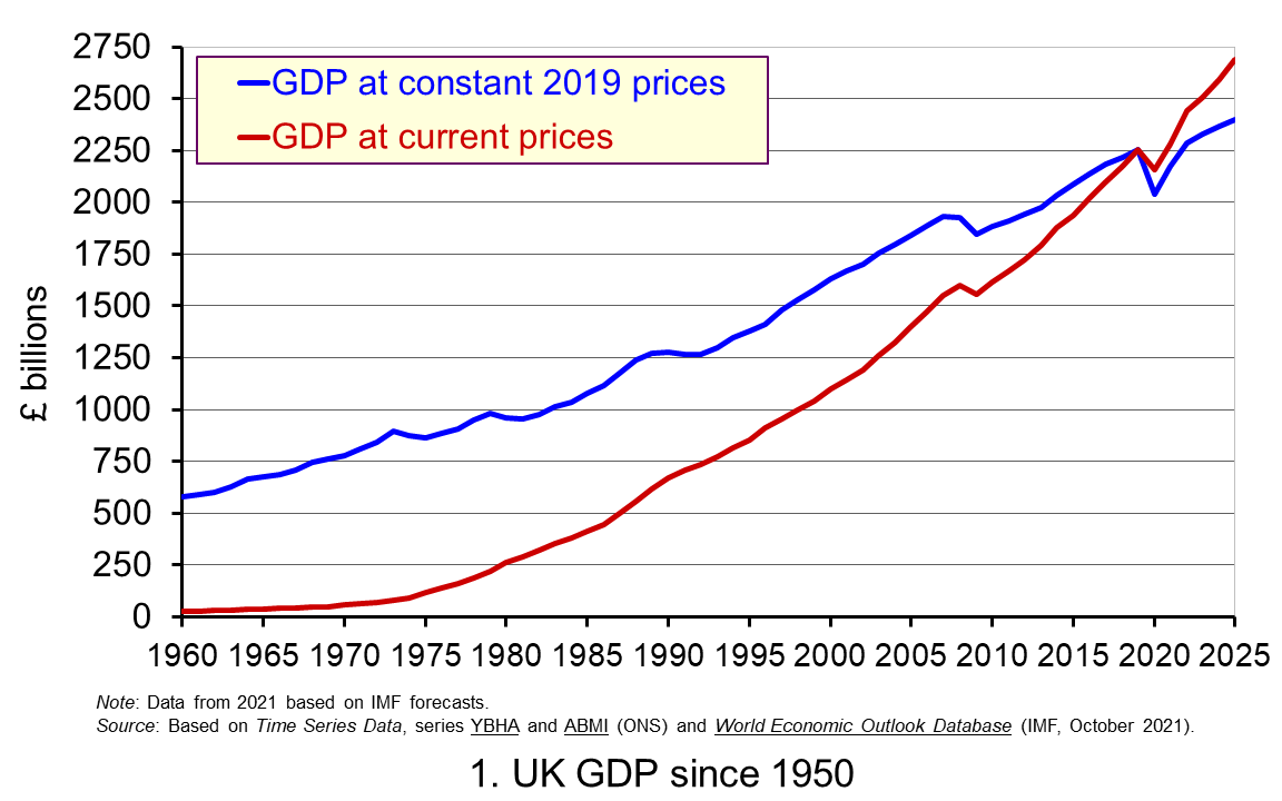 Chart 1 shows current-price estimates of GDP from 1950 when the value of GDP was estimated at £12.7 billion. The increase to £2.156 trillion in 2020 amounts to a proportionate increase of almost 170 times, a figure that rises to 211 times if we compare the 1950 value with the latest IMF estimate for 2025 of £2.689 trillion. However, if we want to make a more meaningful comparison of the country’s national income by looking at the longer-term increase in the volume of production, we need to adjust for inflation. (Click
 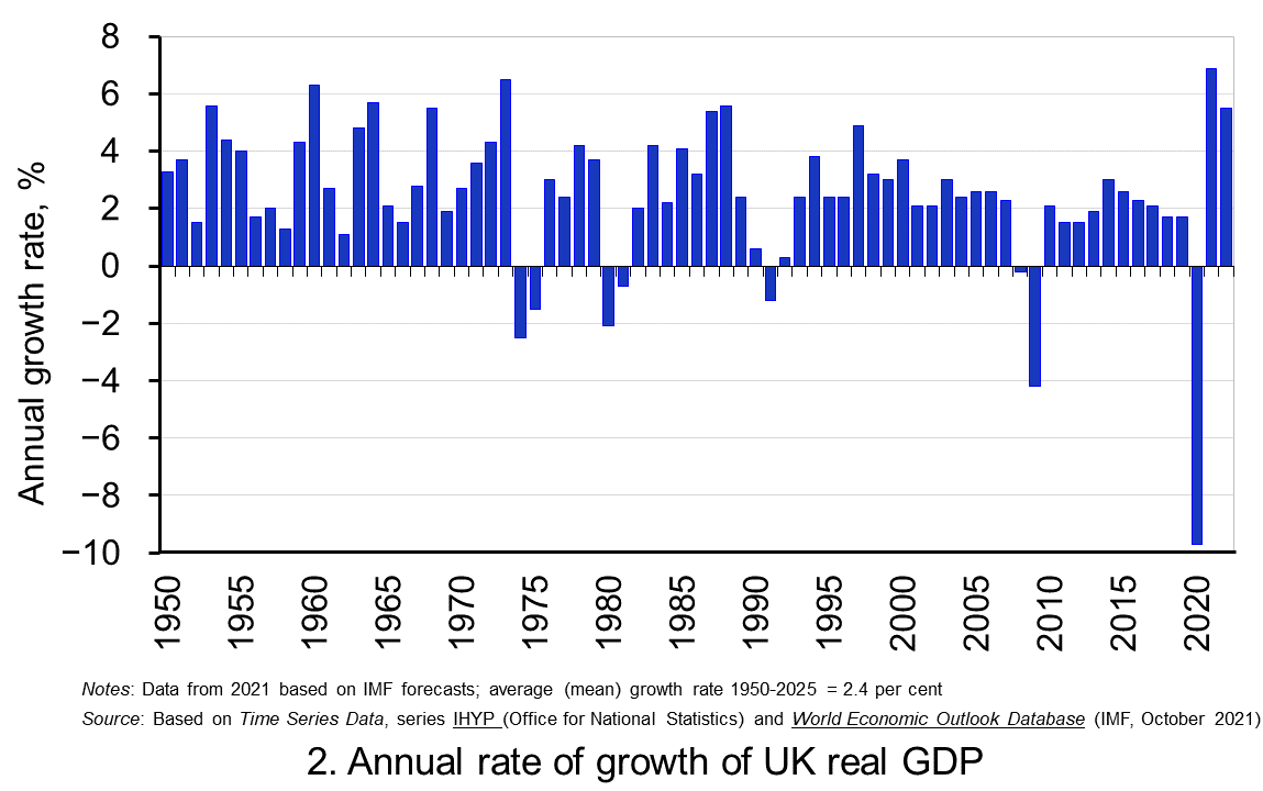 Chart 2 shows the annual rate of growth in real GDP each year since 1950. From it, we see the inherent instability that is a key characteristic of the macroeconomic environment. This instability is, of course, mirrored in the output path of real GDP in Chart 1, but the annual rates of growth show the instability more clearly. We can readily see the impact on national output of the global financial crisis and the global health emergency.
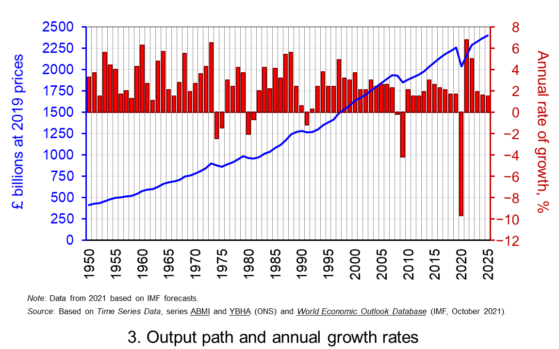 The twin characteristics of growth can be seen simultaneously by combining the output path captured by the levels of real GDP with the annual rates of growth. This is shown in Chart 3. The longer-term growth seen in the economy’s output path is generally argued to be driven by the quantity and quality of the economy’s resources, and their effectiveness when combined in production. In other words, it is the supply-side that determines the trajectory of the output path over the longer term. (Click