 On 25 November, the UK government published its Spending Review 2020. This gives details of estimated government expenditure for the current financial year, 2020/21, and plans for government expenditure and the likely totals for 2021/22.
The focus of the Review is specifically on the effects of and responses to the coronavirus pandemic. It does not consider the effects of Brexit, with or without a trade deal, or plans for taxation. The Review is based on forecasts by the Office for Budget Responsibility (OBR). Because of the high degree of uncertainty over the spread of the disease and the timing and efficacy of vaccines, the OBR gives three forecast values for most variables – pessimistic, central and optimistic.
 According to the central forecast, real GDP is set to decline by 11.3% in 2020, the largest one-year fall since the Great Frost of 1709. The economy is then set to ‘bounce back’ (somewhat), with GDP rising by 5.2% in 2021.
Unemployment will rise from 3.9% in 2019 to a peak of 7.5% in mid-2021, after the furlough scheme and other support for employers is withdrawn.
This blog focuses at the impact on government borrowing and debt and the implications for the future – both the funding of the debt and ways of reducing it.
Soaring government deficits and debt
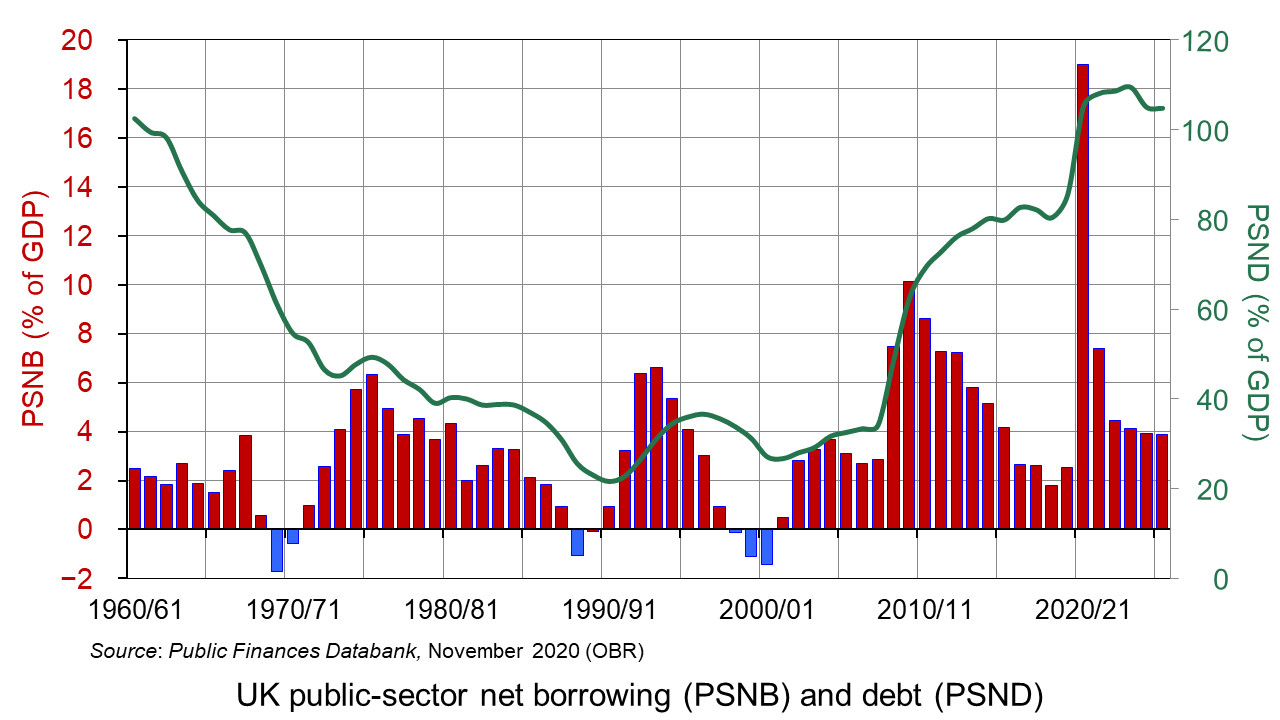
Government expenditure during the pandemic has risen sharply through measures such as the furlough scheme, the Self-Employment Income Support Scheme and various business loans. This, combined with falling tax revenue, as incomes and consumer expenditure have declined, has led to a rise in public-sector net borrowing (PSNB) from 2.5% of GDP in 2019/20 to a central forecast of 19% for 2020/21 – the largest since World War II. By 2025/26 it is still forecast to be 3.9% of GDP. The figure has also been pushed up by a fall in nominal GDP for 2020/21 (the denominator) by nearly 7%. (Click here for a PowerPoint of the above chart.)
The high levels of PSNB are pushing up public-sector net debt (PSNB). This is forecast to rise from 85.5% of GDP in 2019/20 to 105.2% in 2020/21, peaking at 109.4% in 2023/24.
The exceptionally high deficit and debt levels will mean that the government misses by a very large margin its three borrowing and debt targets set out in the latest (Autumn 2016) ‘Charter for Budget Responsibility‘. These are:
- to reduce cyclically-adjusted public-sector net borrowing to below 2% of GDP by 2020/21;
- for public-sector net debt as a percentage of GDP to be falling in 2020/21;
- for overall borrowing to be zero or in surplus by 2025/26.
But, as the Chancellor said in presenting the Review:
Our health emergency is not yet over. And our economic emergency has only just begun. So our immediate priority is to protect people’s lives and livelihoods.
Putting the public finances on a sustainable footing
Running a large budget deficit in an emergency is an essential policy for dealing with the massive decline in aggregate demand and for supporting those who have, or otherwise would have, lost their jobs. But what of the longer-term implications? What are the options for dealing with the high levels of debt?
1. Raising taxes. This tends to be the preferred approach of those on the left, who want to protect or improve public services. For them, the use of higher progressive taxes, such as income tax, or corporation tax or capital gains tax, are a means of funding such services and of providing support for those on lower incomes. There has been much discussion of the possibility of finding a way of taxing large tech companies, which are able to avoid taxes by declaring very low profits by diverting them to tax havens.
2. Cutting government expenditure. This is the traditional preference of those on the right, who prefer to cut the overall size of the state and thus allow for lower taxes. However, this is difficult to do without cutting vital services.  Indeed, there is pressure to have higher government expenditure over the longer term to finance infrastructure investment – something supported by the Conservative government.
A downside of either of the above is that they squeeze aggregate demand and hence may slow the recovery. There was much discussion after the financial crisis over whether ‘austerity policies’ hindered the recovery and whether they created negative supply-side effects by dampening investment.
3. Accepting higher levels of debt into the longer term. This is a possible response as long as interest rates remain at record low levels. With depressed demand, loose monetary policy may be sustainable over a number of years. Quantitative easing depresses bond yields and makes it cheaper for governments to finance borrowing. Servicing high levels of debt may be quite affordable.
The problem is if inflation begins to rise. Even with lower aggregate demand, if aggregate supply has fallen faster because of bankruptcies and lack of investment, there may be upward pressure on prices. The Bank of England may have to raise interest rates, making it more expensive for the government to service its debts.
Another problem with not reducing the debt is that if another emergency occurs in the future, there will be less scope for further borrowing to support the economy.
 4. Higher growth ‘deals’ with the deficit and reduces debt. In this scenario, austerity would be unnecessary. This is the ‘golden’ scenario – for the country to grow its way out of the problem. Higher output and incomes leads to higher tax revenues, and lower unemployment leads to lower expenditure on unemployment benefits. The crucial question is the relationship between aggregate demand and supply. For growth to be sustainable and shrink the debt/GDP ratio, aggregate demand must expand steadily in line with the growth in aggregate supply. The faster aggregate supply can grow, the faster can aggregate demand. In other words, the faster the growth in potential GDP, the faster can be the sustainable rate of growth of actual GDP and the faster can the debt/GDP ratio shrink.
One of the key issues is the degree of economic ‘scarring’ from the pandemic and the associated restrictions on economic activity. The bigger the decline in potential output from the closure of firms and the greater the deskilling of workers who have been laid off, the harder it will be for the economy to recover and the longer high deficits are likely to persist.
Another issue is the lack of labour productivity growth in the UK in recent years. If labour productivity does not increase, this will severely restrict the growth in potential output. Focusing on training and examining incentives, work practices and pay structures are necessary if productivity is to rise significantly. So too is finding ways to encourage firms to increase investment in new technologies.
Podcast and videos
Articles
- Initial reaction from IFS researchers on Spending Review 2020 and OBR forecasts
IFS Press Release, Paul Johnson, Carl Emmerson, Ben Zaranko, Tom Waters and Isabel Stockton (25/11/200
- Rishi Sunak is likely to increase spending – which means tax rises will follow
IFS, Newspaper Article, Paul Johnson (23/11/20)
- Economic and Fiscal Outlook Executive Summary
OBR (25/11/20)
- UK’s Sunak says public finances are on ‘unsustainable’ path
Reuters, David Milliken (26/11/20)
- Rishi Sunak warns ‘economic emergency has only just begun’
BBC News, Szu Ping Chan (25/11/20)
- UK will need £27bn of spending cuts or tax rises, watchdog warns
The Guardian, Phillip Inman (25/11/20)
- What is tomorrow’s Spending Review all about?
The Institute of Chartered Accountants in England and Wales (24/11/20)
- Spending Review 2020: the experts react
The Conversation, Drew Woodhouse, Ernestine Gheyoh Ndzi, Jonquil Lowe, Anupam Nanda, Alex de Ruyter and Simon J. Smith (25/11/20)
OBR Data
Questions
- What is the significance of the relationship between the rate of economic growth and the rate of interest for financing public-sector debt over the longer term?
- What can the government do to encourage investment in the economy?
- Using OBR data, find out what has happened to the output gap over the past few years and what is forecast to happen to it over the next five years. Explain the significance of the figures.
- Distinguish between demand-side and supply-side policies. How would you characterise the policies to tackle public-sector net debt in terms of this distinction? Do the policies have a mixture of demand- and supply-side effects?
- Choose two other developed countries. Examine how their their public finances have been affected by the coronavirus pandemic and the policies they are adopting to tackle the economic effects of the pandemic.
 In recent years, US tech companies have faced increased scrutiny in Washington over their size and power. Despite the big tech firms in America being economically robust, seemingly more so than any other sector, they are also more politically vulnerable. This potential vulnerability is present regardless of the recent election result.
Both the Democrat and Republican parties are thinking critically about monopoly power and antitrust issues, where ‘antitrust’ refers to the outlawing or control of oligopolistic collusion. Despite the varied reasons across different parts of the political spectrum, the increased scrutiny over big tech companies is bipartisan.
Rising monopoly power
Monopoly power occurs when a firm has a dominant position in the market. A pure monopoly is when one firm has a 100% share of the market. A firm might be considered to have monopoly power with more than a 25% market share.
If there is a rise in market concentration, it tends to hurt blue-collar workers, such as those employed in factories, more than everyone else. Research, from the University of Chicago, studied what happens to particular classes of workers when companies increasingly dominate a market and have more power to raise prices. The study found that those workers that make things tend to be left worse off, while the workers who sell, market or design things gain. When companies have more pricing power, they make fewer products and sell each one for a higher profit margin. In that case, it’s far more valuable to a company to be an employee working in so-called expansionary positions, such as marketing, than in production jobs, such as working on a factory line — because there’s less production to be done and more salesmanship.
Monopoly power under Trump Vs Biden
 In February, President Trump and his economic team saw no need to rewrite the federal government’s antitrust rules, drawing a battle line with the Democrats on an issue that has increasingly drawn the attention of economists, legal scholars and other academics. In their annual Economic Report of the President, Mr. Trump and his advisers effectively dismissed research that found large American companies increasingly dominate industries like telecommunications and tech, stifling competition and hurting consumers. At the time the Trump administration contended that studies demonstrating a rise in market concentration were flawed and that the rise of large companies may not be a bad thing for consumers.
On page 201, the report reads:
Concentration may be driven by economies of scale and scope that can lower costs for consumers. Also, successful firms tend to grow, and it is important that antitrust enforcement and competition policy not be used to punish firms for their competitive success.
The Trump administration approved some high-profile corporate mergers, such as the merger of Sprint and T-Mobile, while also trying to block others, such as AT&T’s purchase of Time Warner. Mr. Trump’s advisers stated that agencies already had the tools they needed to evaluate mergers and antitrust cases. It lamented that some Americans have come to hold the mistaken, simplistic view that ‘Big Is Bad.’
However, it is likely that such big firms, including the tech giants, would take a hit under the new presidency. President-Elect Joe Biden has pledged to undo the tax cuts introduced by Trump and has vowed to increase corporation tax from 21% to 28%. As part of these tax changes, he has suggested the introduction of a minimum 15% tax for all companies with a revenue of over $100 million. This has now been given the nickname of the ‘Amazon Tax’ and it is clear how it would impact on the big the firms such as Amazon.
This is the opposite of what was probable if Trump were to have been re-elected. It was expected that the US would continue along the path of deregulation and lower taxes for corporates and high-income households, which would have been welcomed by the stock market. However, analysts suggest that the tax changes under Biden would negatively affect the US tech sector, with some analysts maintaining that the banking sector would also be hit.
 Antitrust enforcement is often associated with the political left, but the current situation is not so clear-cut. In the past, Silicon Valley has largely avoided any clashes with Washington, even when European regulators have levied fines against the tech giants. European regulators have fined Google a total of $9bn for anticompetitive practices. In 2018 Donald Trump attacked the EU decisions. “I told you so! The European Union just slapped a Five Billion Dollar fine on one of our great companies, Google,” Trump tweeted. “They truly have taken advantage of the US, but not for long!”
However, since then the mood has changed, with Trump and other conservatives joining liberals, including senators Elizabeth Warren and Bernie Sanders, in attacking the dominance of tech firms, including Amazon, Google, Facebook and others. While Democrats have largely stuck to criticising the scale of big tech’s dominance, Republicans, including Trump, have accused the major tech companies of censoring conservative speech.
An antitrust subcommittee of the Democrat-controlled House Judiciary Committee released a 449-page report excoriating the Big Four tech companies, Amazon, Facebook, Apple and Google-owner, Alphabet, for what it calls systematic and continuing abuses of their monopoly power. Recommendations from the report include ways to limit their power, force them out of certain areas of business and even a break-up of some of them.
Democratic lawmakers working on the probe claim that these firms have too much power, and that power must be reined in. But not all Republicans involved agreed with the recommendations. One Republican congressman, Jim Jordan, dismissed the report as “partisan” and said it advanced “radical proposals that would refashion antitrust law in the vision of the far left.” However, others have said they support many of the report’s conclusions about the firms’ anti-competitive tactics, but that remedies proposed by Democrats go too far.
The US tech giants

Amazon is a leading example of the economic strength held by the tech giants. Amazon has produced 12-month revenues of $321bn to October 2020, which in an increase from 2019 and 2018 revenues of $280bn and $233bn respectively. However, Amazon, along with the other big players Apple, Facebook, Google parent Alphabet, and Microsoft, are facing increased government scrutiny.
The US Department of Justice has filed a lawsuit against Google for entrenching itself as the dominant search engine through anti-competitive practices. Google’s complex algorithms, software, and custom-built servers helped make it into one of the world’s richest and most-powerful corporations. It currently dominates the online search market in the USA, accounting for around 80% of search queries. The lawsuit accuses the tech company of abusing its position to maintain an illegal monopoly over search and search advertising. Facebook also faces an antitrust lawsuit from the Federal Trade Commission. It is arguable that the US tech giants are so powerful that they may accomplish the seemingly impossible and unite the two parties, at least on one policy – breaking them up.
If it is correct that the tech giants’ behaviour ultimately damages innovation and exacerbates inequality, it is arguable that such problems have only grown worse with the coronavirus pandemic. Many smaller businesses have succumbed to the economic damage: many have been closed during lockdowns or suffered a decline in sales; many have gone out of business.
The changing patterns in teleworking and retail have accelerated in ways that have made Americans more reliant on technologies produced by a few firms. Shares in the Big Four, along with Microsoft, Netflix, and Tesla, added $291 billion in market value in just one day last week. It could therefore be claimed that the dangers of Big Tech domination are more profound now than they were even a few months ago.
Google’s lawsuit
On 20 October, the Department of Justice — along with eleven state Attorneys General — filed a civil antitrust lawsuit in the U.S. District Court for the District of Columbia to stop Google from unlawfully maintaining monopolies through anticompetitive and exclusionary practices in the search and search advertising markets and to remedy the competitive harms.
 This is the most significant legal challenge to a major tech company in decades and comes as US authorities are increasingly critical of the business practices of the major tech companies. The suit alleges that Google is no longer a start-up company with an innovative way to search the emerging internet. Instead Google is being described as a “monopoly gatekeeper for the internet” that has used “pernicious” anticompetitive tactics to maintain and extend its monopolies.
The allegation that Google is unfairly acting as a gatekeeper to the internet is based on the argument that through a series of business agreements, Google has effectively locked out any competition. One of the specific arrangements being challenged is the issue of Google being preloaded on mobile devices. On mobile phones running its Android operating system, Google is preinstalled and cannot be deleted. The company pays billions each year to “secure default status for its general search engine and, in many cases, to specifically prohibit Google’s counterparties from dealing with Google’s competitors,” the suit states. It is argued that this alone forecloses competition for internet search as it denies its rivals to compete effectively and prevent potential innovation.
However, Google has defended its position, calling the lawsuit “deeply flawed”. It has argued that consumers themselves choose to use Google; they do not use it because they are forced to or because they can’t find an alternative search platform. Google also argues that this lawsuit will not be beneficial for consumers. It claims that this will artificially prop up lower-quality search alternatives, increase phone prices, and make it harder for people to get the search services they want to use.
Conclusion
Despite wanting to stop Google from “unlawfully maintaining monopolies in the markets for” search services, advertising, and general search text, the lack of consensus and divergence among the Democrats and Republicans on the antitrust issues remains a major issue to move things forward.
The Democrats want to see the power held by these companies reined in, while the Republicans would rather see targeted antitrust enforcement over onerous and burdensome regulation that kills industry innovation. It is clear that the US government will have to balance its reforms and ideas while making sure not to put the largest companies in the USA at a competitive disadvantage versus their competitors globally.
Articles
- US tech giants accused of ‘monopoly power’
BBC News (6/10/20)
- Tech, healthcare & the ‘fear index’: An investor’s guide to US election night 2020
Investment Trust Insider, Alex Steger, Alex Rosenberg, John Coumarianos, Nicole Piper, Jake Martin and Ian Wenik (2/11/20)
- Justice Department Sues Monopolist Google For Violating Antitrust Laws
The United States Department of Justice (20/10/20)
- Trump Administration Sees No Threat to Economy From Monopolies
The New York Times, Jim Tankersley (20/2/20)
- Trump vs Biden: Winners and losers under America’s next leader
Shares, Yoosof Farah (29/10/20)
- America’s Monopoly Problem Goes Way Beyond the Tech Giants
The Atlantic, David Dayen (28/7/20)
- US justice department sues Google over accusation of illegal monopoly
The Guardian, Dominic Rushe and Kari Paul (20/10/20)
Questions
- With the aid of a diagram, explain how pricing decisions are made in a monopoly.
- What factors influence the degree of monopoly power a company has within an industry?
- What are the advantages of a monopoly?
- Why would a government want to prevent a monopoly? Discuss the policies a government could implement to do this.
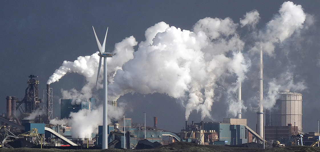
With the election of Joe Biden, the USA will have a president committed to tackling climate change. This is in stark contrast to Donald Trump, who has been publicly sceptical about the link between human action and climate change and has actively supported the coal, oil and gas industries and has rolled back environmental protection legislation and regulation.
 What is more, in June 2017, he announced that the USA would withdraw from the UN Paris Accord, the international agreement to cut greenhouse gas emissions so as to limit global warming to ‘well below’ 2°C above pre-industrial levels with efforts to limit it to 1.5°C. The USA’s withdrawal was finalised on 4 November 2020, a day after the US election. Joe Biden, however, pledged to rejoin the accord.
A growing number of countries are pledging to achieve carbon neutrality by mid-century or earlier. The EU is planning to achieve a 55% cut in greenhouse gas emissions by 2030 so as to reach neutrality by 2050. This will involve various taxes, subsidies and public investment. Similar pledges to achieve net zero emissions by 2050 have been made by Japan and South Korea and by 2060 by China. In the UK, legislation was passed requiring the government to reduce the UK’s net emissions 100% relative to 1990 levels by 2050 and thereby achieve net zero emissions.
Constraints on action
Short-termism. One of the problems with setting targets a long time in the future is that they take away the urgency to act now. There are huge time lags between introducing policies to curb carbon emissions and their impact on the climate. The costs of such policies for business and consumers, however, are felt immediately in terms of higher taxes and/or higher prices. Thus politicians may be quick to make long-term pledges but reluctant to take firm measures today. Instead they may prefer to appease various pressure groups, such as motoring organisations, and cut fuel taxes, or, at least, not raise them. Politically, then, it may be easier to focus policy on the short term and just make pledges without action for the future.
Externalities. Various activities that cause carbon emissions, whether directly, such as heavy industry, dairy farming, aviation and shipping, or indirectly, such as oil and coal production, thereby impose environmental costs on society, both at home and abroad. These costs are negative externalities and, by their nature, are not borne by those who produce them. There are often powerful lobbies objecting to any attempt to internalise these externalities through taxes, subsidising green alternatives or regulation. Take the case of the USA. Fossil fuel producers, energy-intensive industries and farmers all claim that green policies will damage their businesses, leading to a loss of profits and jobs. These groups were courted by Donald Trump.

International competition. Countries may well be reluctant to impose green taxes or tough environmental regulation on producers, when competitors abroad do not face such constraints. Indeed, some countries are actively promoting dirty industries as part of their policies to stimulate economic recovery from the Covid-induced recession. Such countries include China, Russia and Turkey. This again was a major argument used in the Trump campaign that US industries should not be hobbled by environmental constraints but should be free to compete.
Misinformation. Politicians, knowing that taking tough environmental measures will be unpopular with large numbers of people, may well downplay the dangers of inaction. Some, such as Trump in America and Bolsonaro in Brazil deliberately appeal to climate change deniers or say that technology will sort things out. This makes it hard for other politicians to promote green policies, knowing that they will face scepticism about the science and the efficacy of their proposed policies.
Biden’s climate change policy
 Although it will be difficult to persuade some Americans of the need for tougher policies to tackle climate change, Joe Biden has already made a number of pledges. He has stated that under his administration, the USA will rejoin the Paris Climate Agreement and will play a leading role in the November 2021 UN COP26 climate change conference summit in Glasgow. He has also pledged a Clean Energy Revolution to put the USA on an ‘irreversible path to achieve economy-wide net-zero emissions no later than 2050’.
But readopting the pledges under the Paris Agreement and advocating a clean energy revolution are not enough on their own. Specific measures will need to be taken. So, what can be done that is practical and likely to meet with the approval of the majority of Americans or, at least, of Biden’s supporters?
For a start, he can reintroduce many of the regulations that were overturned by the Trump administration, such as preventing oil and gas companies from flaring methane on public lands. He could introduce funding for the development of green technology. He could require public buildings to use green energy.
According to the Clean Energy Revolution, the US government will develop ‘rigorous new fuel economy standards aimed at ensuring 100% of new sales for light- and medium-duty vehicles will be zero emissions and annual improvements for heavy duty vehicles’.
 One of the biggest commitments is to tackle external costs directly by enacting ‘legislation requiring polluters to bear the full cost of their climate pollution’. This may be met with considerable resistance from US corporations. It is thus politically important for Biden to stress the short-term benefits of his policies, not just the long-term ones.
Given the damage done to the economy by the spread of the pandemic, perhaps the main thing that Biden can do to persuade people of the benefits to them of his policies is to focus on green investment and green jobs. Building a green energy infrastructure of wind, solar and hydro and investing in zero-emissions vehicles and charging infrastructure will provide jobs and lead to multiplier effects throughout the economy.
Articles
- Trump Administration Removes Scientist in Charge of Assessing Climate Change
The New York Times, Christopher Flavelle, Lisa Friedman and Coral Davenport (9/11/20)
- As U.S. leaves Paris accord, climate policy hangs on election outcome
The Washington Post, Brady Dennis, Juliet Eilperin and Dino Grandoni (5/11/20)
- Where next for US action on Climate Change?
British Foreign Policy Group, Evie Aspinall (11/11/20)
- Media reaction: What Joe Biden’s US election victory means for climate change
Carbon Brief, Josh Gabbatiss (10/11/20)
- Joe Biden: How the president-elect plans to tackle climate change
BBC News, Matt McGrath (10/11/20)
- Biden victory ushers in ‘race to the top’ on climate change
Lexology, Baker McKenzie, David P Hackett and Ilona Millar (13/11/20)
- Climate heroes: the countries pioneering a green future
The Guardian, Jonathan Watts (11/11/20)
- ‘Hypocrites and greenwash’: Greta Thunberg blasts leaders over climate crisis
The Guardian, Damian Carrington (9/11/20)
- Five post-Trump obstacles to a global green recovery
The Guardian, Jonathan Watts (11/11/20)
- Biden’s climate change plans can quickly raise the bar, but can they be transformative?
The Conversation, Edward R Carr (10/11/20)
- Jana Shea/Shutterstock Climate change: Joe Biden could ride a wave of international momentum to break deadlock in US
The Conversation, Richard Beardsworth and Olaf Corry (10/11/20)
- Climate change after COVID-19: Harder to defeat politically, easier to tackle economically
VoxEU, Franziska Funke and David Klenert (17/8/20)
Questions
- Identify three specific climate change policies of Joe Biden and assess whether each one is likely to succeed.
- Draw a diagram to illustrate why a free market will lead to over production of a good which produces negative externalities.
- To what extent can education internalise the positive externalities of green consumption and production?
- What was agreed at the Paris climate change conference in December 2015 and what mechanisms were put in place to incentivise countries to meet the targets?
- Will the coronavirus pandemic have had any lasting effects on emissions? Explain.
- How may carbon trading lead to a reduction in carbon emissions? What determines the size of such reductions?
 With the imposition of a new lockdown in England from 5 November to 2 December and in Wales from 3 October to 9 November, and with strong restrictions in Scotland and Northern Ireland, the UK economy is set to return to negative growth – a W-shaped GDP growth curve.
With the closure of leisure facilities and non-essential shops in England and Wales, spending is likely to fall. Without support, many businesses would fail and potential output would fall. In terms of aggregate demand and supply, both would decline, as the diagram below illustrates. (Click here for a PowerPoint.)
The aggregate demand curve shifts from AD1 to AD2 as consumption and investment fall. Exports also fall as demand is hit by the pandemic in other countries. 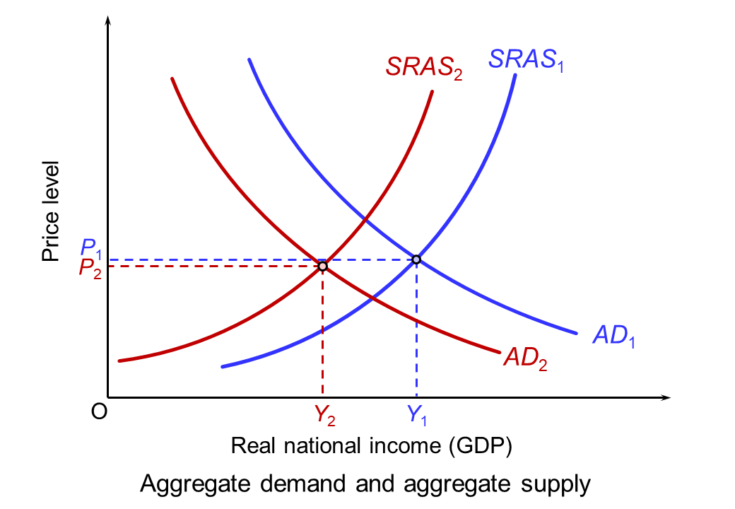 The fall in aggregate supply is represented partly by a movement along the short-run aggregate supply curve (SRAS) as demand falls for businesses which remain open (such as transport services). Largely it is represented by a leftward shift in the curve from SRAS1 to SRAS2 as businesses such as non-essential shops and those in the hospitality and leisure sector are forced to close. What happens to the long-run supply curve depends on the extent to which businesses reopen when the lockdown and any other subsequent restrictions preventing their reopening are over. It also depends on the extent to which other firms spring up or existing firms grow to replace the business of those that have closed. The continuing rise in online retailing is an example.
With the prospect of falling GDP and rising unemployment, the UK government and the Bank of England have responded by giving a fiscal and monetary boost. We examine each in turn.
Fiscal policy
 In March, the Chancellor introduced the furlough scheme, whereby employees temporarily laid off would receive 80% of their wages through a government grant to their employers. This scheme was due to end on 31 October, to be replaced by the less generous Job Support Scheme (see the blog, The new UK Job Support Scheme: how much will it slow the rise in unemployment?). However, the Chancellor first announced that the original furlough scheme would be extended until 2 December for England and then, on 5 November, to the end of March 2021 for the whole of the UK. He also announced that the self-employed income support grant would increase from 55% to 80% of average profits up to £7500.
In addition, the government announced cash grants of up to £3000 per month for businesses which are closed (worth more than £1 billion per month), extra money to local authorities to support businesses and an extension of existing loan schemes for business. Furthermore, the government is extending the scheme whereby people can claim a repayment ‘holiday’ for up to 6 months for mortgages, personal loans and car finance.
The government hopes that the boost to aggregate demand will help to slow, or even reverse, the predicted decline in GDP. What is more, by people being put on furlough rather than being laid off, it hopes to slow the rise in unemployment.
Monetary policy
At the meeting of the Bank of England’s Monetary Policy Committee on 4 November, further expansionary monetary policy was announced. Rather than lowering Bank Rate from its current historically low rate of 0.1%, perhaps to a negative figure, it was decided to engage in further quantitative easing.
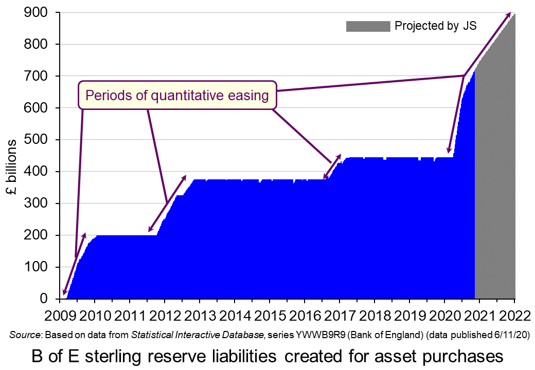 An additional £150 billion of government bonds will be purchased under the asset purchase facility (APF). This will bring the total vale of bonds purchased since the start of the pandemic to £450 billion (including £20 billion of corporate bonds) and to £895 billion since 2009 when QE was first introduced in response to the recession following the financial crisis of 2007–8.
The existing programme of asset purchases should be complete by the end of December this year. The Bank of England expects the additional £150 billion of purchases to begin in January 2021 and be completed within a year.
UK quantitative easing since the first round in March 2009 is shown in the chart above. The reserve liabilities represent the newly created money for the purchase of assets under the APF programme. (There are approximately £30 billion of other reserve liabilities outside the APF programme.) The grey area shows projected reserve liabilities to the end of the newly announced programme of purchases, by which time, as stated above, the total will be £895 billion. This, of course, assumes that the Bank does not announce any further QE, which it could well do if the recovery falters.
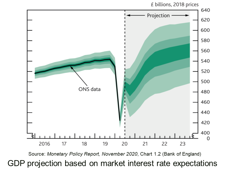
Justifying the decision, the MPC meeting’s minutes state that:
There are signs that consumer spending has softened across a range of high-frequency indicators, while investment intentions have remained weak. …The fall in activity over 2020 has reflected a decline in both demand and supply. Overall, there is judged to be a material amount of spare capacity in the economy.
Conclusions
How effective these fiscal and monetary policy measures will be in mitigating the effects of the Covid restrictions remains to be seen. A lot will depend on how successful the lockdown and other restrictions are in slowing the virus, how quickly a vaccine is developed and deployed, whether a Brexit deal is secured, and the confidence of both consumers, businesses and financial markets that the economy will bounce back in 2021. As the MPC’s minutes state:
The outlook for the economy remains unusually uncertain. It depends on the evolution of the pandemic and measures taken to protect public health, as well as the nature of, and transition to, the new trading arrangements between the European Union and the United Kingdom. It also depends on the responses of households, businesses and financial markets to these developments.
Articles
- Covid: Rishi Sunak to extend furlough scheme to end of March
BBC News (6/11/20)
- Furlough extended until March and self-employed support boosted again
MSE News, Callum Mason (6/11/20)
- Number on furlough in UK may double during England lockdown
The Guardian, Richard Partington (3/11/20)
- ‘We wouldn’t manage without it’: business owners on the furlough extension
The Guardian, Molly Blackall and Mattha Busby (6/11/20)
- Sunak’s abrupt turn on UK furlough scheme draws criticism from sceptics
Financial Times, Delphine Strauss (6/11/20)
 Coronavirus: Bank of England unleashes further £150bn of support for economy
Sky News, James Sillars (5/11/20)
- Bank of England boss pledges to do ‘everything we can’
BBC News, Szu Ping Chan (6/11/20)
- Savers are spared negative rates but the magic money tree delivers £150bn more QE: What the Bank of England’s charts tell us about the economy
This is Money, Simon Lambert (5/11/20)
- Covid-19 and the victory of quantitative easing
The Spectator, Bruce Anderson (26/10/20)
- Will the Bank of England’s reliance on quantitative easing work for the UK economy?
The Conversation, Ghulam Sorwar (9/11/20)
- With a W-shaped recession looming and debt piling up, the government should start issuing GDP-linked bonds
LSE British Politics and Policy blogs, Costas Milas (6/11/20)
Official documents
Questions
- Illustrate the effects of expansionary fiscal and monetary policy on (a) a short-run aggregate supply and demand diagram; (b) a long-run aggregate supply and demand diagram.
- In the context of the fiscal and monetary policy measures examined in this blog, what will determine the amount that the curves shift?
- Illustrate on a Keynesian 45° line diagram the effects of (a) the lockdown and (b) the fiscal and monetary policy measures adopted by the government and Bank of England.
- If people move from full-time to part-time working, how is this reflected in the unemployment statistics? What is this type of unemployment called?
- How does quantitative easing through asset purchases work through the economy to affect output and employment? In other words, what is the transmission mechanism of the policy?
- What determines the effectiveness of quantitative easing?
- Under what circumstances will increasing the money supply affect (a) real output and (b) prices alone?
- Why might quantitative easing benefit the rich more than the poor?
- How could the government use quantitative easing to finance its budget deficit?
The UK rail industry was privatised by the Conservative government in the mid-1990s. As Case Study 14.8 on the Economics 10th edition website states:
 The management of rail infrastructure, such as track, signalling and stations, was to be separated from the responsibility for running trains. There would be 25 passenger train operating companies (TOCs), each having a franchise lasting between seven and fifteen years. These companies would have few assets, being forced to rent track and lease stations from the infrastructure owner (Railtrack), and to lease trains and rolling stock from three new rolling-stock companies. …In practice, the 25 franchises were operated by just 11 companies (with one, National Express, having nine of the franchises).
In 1996, at the start of the franchise era, the train operating companies were largely private-sector companies such as National Express, Stagecoach, Virgin Rail and Prism Rail. By 2020, most of the franchises were operated by a foreign state-owned business or a joint venture with a foreign state-owned firm.
As a result of poor performance (see above case study), Railtrack was effectively renationalised in 2002 as Network Rail – a not-for-profit company, wholly dependent upon the UK Treasury for any shortfall in its funds.
TOCs had mixed success. Some performed so poorly that their franchise contracts had to be temporarily taken over by a state-owned operator. For example, in June 2003 the Strategic Rail Authority withdrew the operating licence of the French company Connex South Eastern. The franchise was temporarily taken over by the publicly-owned South Eastern Trains from November 2003 until March 2006 before being returned to a private operator.
Perhaps the most troubled franchise has been the East Coast Main Line between London and Scotland. It was renationalised in 2009, reprivatised in 2015 and renationalised in 2018.
The effect of the coronavirus pandemic
 The spread of the coronavirus and the accompanying lockdowns and social distancing saw a plummeting of rail travel. Passenger numbers fell to just 10% of pre-pandemic levels. In March 2020, the UK Government introduced Emergency Measures Agreements (EMAs), which temporarily replaced rail franchise agreements. TOCs were paid a 2% fee (based on pre-Covid costs) to run trains and losses were borne by the government.
When the EMAs ran out on the 20 September, they were replaced by Emergency Recovery Measures Agreements (ERMAs), set to last until no later than April 2022. Under these measures, the fees paid to TOCs were reduced to a maximum of 1.5%. These consist partly of a fixed fee (again based on pre-Covid costs) and partly on a performance payment, depending on punctuality, passenger satisfaction and financial performance. As with the EMAs, the new arrangements involve virtually no risk for the TOCs (except for the size of the performance-related fee). Costs and revenue will be passed to the Department for Transport, which will bear any losses.
TOCs were required to run a virtually full service to allow reduced passenger numbers to observe social distancing. Despite journeys still being only 30% of pre-pandemic levels, social distancing on trains meant that many trains were sold out.
 The ERMAs also contain provisions for the replacement of franchises when they come to an end. The precise nature of these will be spelt out in a White Paper, which will respond to the recommendations of the Williams Review of the railways. This review was set up in 2018 in the aftermath of difficulties with various franchises and a chaotic nationwide timetable change. The review’s findings were originally scheduled to be published in Autumn 2019, but were then put back because of the general election and the disruptions caused by the pandemic. The government hopes that it will be published before the end of 2020.
It is expected that the review will recommend replacing the franchise system with something similar to the currents ERMAs. TOCs awarded a contract will be paid a performance-related fee and revenues will go to the government, which will bear the costs. While this is not quite renationalisation, it is not the previous franchise system where TOCs bore the risks. It is in effect a contract system where private companies are paid to deliver a public service.
The CrossCountry franchise
 The first test of this new approach to contracting with TOCs came this month. Arriva’s franchise for running CrossCountry trains ran out and was replaced by a three-year contract to run the services, which span
  much of the length of Great Britain from Aberdeen to Penzance via Edinburgh, Glasgow, Newcastle, Sheffield, Birmingham, Bristol and Plymouth; from Bournemouth to Manchester via Reading, Oxford, Wolverhampton and Stoke; from Cardiff to Nottingham via Gloucester, Birmingham and Derby; and from Birmingham to Stanstead Airport via Leicester and Cambridge.
The contract will last three years. The Department for Transport will gain the revenues and cover the costs and pay Arriva (owned by Deutsche Bahn) a management fee that is ‘performance related’ – as yet unspecified. This, like the EMAs and then the ERMAs, will remove the risks from Arriva.
Nationalisation in Wales
 The Welsh government has announced that Transport for Wales will be taken over by a publicly owned company in February 2021. TfW operates many of the routes in Wales and the borders and most of the branch lines in Wales, including the valley commuter lines into Cardiff. It is currently owned by KeolisAmey (a joint company owned 70% by the French company, Keolis (part of SNCF), and 30% by the UK company, Amey), which took over the franchise in 2018 from Arriva. The Welsh government considered that KeolisAmey would collapse if it did not provide support. Ministers decided that nationalisation would give it greater control than simply subsidising KeolisAmey.
James Price, chief executive of the Welsh Government, stated that this allows it:
to reduce the profit we pay to the private sector massively over time, and make sure that when the revenue comes back, it comes back in to the taxpayer.
Under emergency measures, KeolisAmey has already been supported by the Welsh government to the tune of £105 million (£40 million in March and £65 million in June) to continue operating the franchise. Passenger numbers fell by 95% as the pandemic hit.
Is nationalisation a better way forward, or should private train operating companies continue with the government taking on the risks, or should the franchise system be amended with greater support from the government but with the TOCs still bearing risk? The articles below consider these issues.
Articles
- Rail nationalisations may be coming down the track
BBC News, Tom Burridge (17/9/20)
- ONS recognises full nationalisation of the UK railways
Financial Times, Tanya Powley (31/7/20)
- Train services are very efficient for shareholders – less so for customers
The Conversation, Daniel Fisher (22/8/19)
- UK government on standby to nationalise more rail lines
Financial Times, Jim Pickard and Philip Georgiadis (17/9/20)
- British Government Ends Rail Franchising
Railway-News, Josephine Cordero Sapién (21/9/20)
- British government announces end for rail franchise system
Trains, Keith Fender (12/10/20)
- Monday essay: A new era?
Railnews, Sim Harris (19/10/20)
- Arriva secures three-year CrossCountry contract
International railway Journal Kevin Smith (16/10/20)
- New contract signed for Arriva CrossCountry
RTM, Ailsa Cowen (16/10/20)
- Franchising is Dead
Railway-News, Josephine Cordero Sapién and Gareth Davies (16/9/20)
- Transport for Wales rail services to be nationalised
BBC News (23/10/20)
- Transport for Wales to be nationalised
Railnews (22/10/20)
- Why has the Welsh Government nationalised rail’s Wales and Borders franchise?
BusinessLive, Sion Barry (22/10/20)
Questions
- Explain how the franchising system worked (prior to March 2020).
- To what extent could each franchise be described as a ‘contestable monopoly’?
- What incentives were built into the franchising system to deliver improvements in service for passengers?
- What were the weaknesses of the franchising system?
- In the context of post-pandemic rail services, compare the relative merits of nationalisation with those of awarding contracts where the government receives the revenues and bears the costs and pays train operating companies a fee for operating the services where the size of the fee is performance related.
- What are the arguments for subsidising rail transport? What should determine the size of the subsidy?
 On 25 November, the UK government published its Spending Review 2020. This gives details of estimated government expenditure for the current financial year, 2020/21, and plans for government expenditure and the likely totals for 2021/22.
  According to the central forecast, real GDP is set to decline by 11.3% in 2020, the largest one-year fall since the Great Frost of 1709. The economy is then set to ‘bounce back’ (somewhat), with GDP rising by 5.2% in 2021.
 Indeed, there is pressure to have higher government expenditure over the longer term to finance infrastructure investment – something supported by the Conservative government.
 4. Higher growth ‘deals’ with the deficit and reduces debt. In this scenario, austerity would be unnecessary. This is the ‘golden’ scenario – for the country to grow its way out of the problem. Higher output and incomes leads to higher tax revenues, and lower unemployment leads to lower expenditure on unemployment benefits. The crucial question is the relationship between aggregate demand and supply. For growth to be sustainable and shrink the debt/GDP ratio, aggregate demand must expand steadily in line with the growth in aggregate supply. The faster aggregate supply can grow, the faster can aggregate demand. In other words, the faster the growth in potential GDP, the faster can be the sustainable rate of growth of actual GDP and the faster can the debt/GDP ratio shrink.
 How Broke is Britain?
 Chancellor Rishi Sunak warns UK economy will shrink by 11% this year
 COVID and beyond: Public finances explained
 Spending Review 2020: IFS Analysis
 In recent years, US tech companies have faced increased scrutiny in Washington over their size and power. Despite the big tech firms in America being economically robust, seemingly more so than any other sector, they are also more politically vulnerable. This potential vulnerability is present regardless of the recent election result.
  In February, President Trump and his economic team saw no need to rewrite the federal government’s antitrust rules, drawing a battle line with the Democrats on an issue that has increasingly drawn the attention of economists, legal scholars and other academics. In their annual
 This is the most significant legal challenge to a major tech company in decades and comes as US authorities are increasingly critical of the business practices of the major tech companies. The suit alleges that Google is no longer a start-up company with an innovative way to search the emerging internet. Instead Google is being described as a “monopoly gatekeeper for the internet” that has used “pernicious” anticompetitive tactics to maintain and extend its monopolies.
 What is more, in June 2017, he announced that
 Although it will be difficult to persuade some Americans of the need for tougher policies to tackle climate change, Joe Biden has already made a number of pledges. He has stated that under his administration, the USA will
  One of the biggest commitments is to tackle external costs directly by enacting ‘legislation requiring polluters to bear the full cost of their climate pollution’. This may be met with considerable resistance from US corporations. It is thus politically important for Biden to stress the short-term benefits of his policies, not just the long-term ones.
 With the imposition of a new lockdown in England from 5 November to 2 December and in Wales from 3 October to 9 November, and with strong restrictions in Scotland and Northern Ireland, the UK economy is set to return to negative growth – a W-shaped GDP growth curve.
  The fall in aggregate supply is represented partly by a movement along the short-run aggregate supply curve (SRAS) as demand falls for businesses which remain open (such as transport services). Largely it is represented by a leftward shift in the curve from SRAS1 to SRAS2 as businesses such as non-essential shops and those in the hospitality and leisure sector are forced to close. What happens to the long-run supply curve depends on the extent to which businesses reopen when the lockdown and any other subsequent restrictions preventing their reopening are over. It also depends on the extent to which other firms spring up or existing firms grow to replace the business of those that have closed. The continuing rise in online retailing is an example.
 In March, the Chancellor introduced the furlough scheme, whereby employees temporarily laid off would receive 80% of their wages through a government grant to their employers. This scheme was due to end on 31 October, to be replaced by the less generous Job Support Scheme (see the blog,
  An additional £150 billion of government bonds will be purchased under the asset purchase facility (APF). This will bring the total vale of bonds purchased since the start of the pandemic to £450 billion (including £20 billion of corporate bonds) and to £895 billion since 2009 when QE was first introduced in response to the recession following the financial crisis of 2007–8.
 The management of rail infrastructure, such as track, signalling and stations, was to be separated from the responsibility for running trains. There would be 25 passenger train operating companies (TOCs), each having a franchise lasting between seven and fifteen years. These companies would have few assets, being forced to rent track and lease stations from the infrastructure owner (Railtrack), and to lease trains and rolling stock from three new rolling-stock companies. …In practice, the 25 franchises were operated by just 11 companies (with one, National Express, having nine of the franchises).
 The spread of the coronavirus and the accompanying lockdowns and social distancing saw a plummeting of rail travel. Passenger numbers fell to just 10% of pre-pandemic levels. In March 2020, the UK Government introduced Emergency Measures Agreements (EMAs), which temporarily replaced rail franchise agreements. TOCs were paid a 2% fee (based on pre-Covid costs) to run trains and losses were
  The ERMAs also contain provisions for the replacement of franchises when they come to an end. The precise nature of these will be spelt out in a White Paper, which will respond to the recommendations of the
  The first test of this new approach to contracting with TOCs came this month. Arriva’s franchise for running CrossCountry trains ran out and was replaced by a three-year contract to run the services,
  much of the length of Great Britain from Aberdeen to Penzance via Edinburgh, Glasgow, Newcastle, Sheffield, Birmingham, Bristol and Plymouth; from Bournemouth to Manchester via Reading, Oxford, Wolverhampton and Stoke; from Cardiff to Nottingham via Gloucester, Birmingham and Derby; and from Birmingham to Stanstead Airport via Leicester and Cambridge.
 The Welsh government has announced that Transport for Wales will be taken over by a publicly owned company in February 2021. TfW operates many of the routes in Wales and the borders and most of the branch lines in Wales, including the valley commuter lines into Cardiff. It is currently owned by