 Both the financial and goods markets are heavily influenced by sentiment. And such sentiment tends to be self-reinforcing. If consumers and investors are pessimistic, they will not spend and not invest. The economy declines and this further worsens sentiment and further discourages consumption and investment. Banks become less willing to lend and stock markets fall. The falling stock markets discourage people from buying shares and so share prices fall further. The despondency becomes irrational and greatly exaggerates economic fundamentals.
This same irrationality applies in a boom. Here it becomes irrational exuberance. A boom encourages confidence and stimulates consumer spending and investment. This further stimulates the boom via the multiplier and accelerator and further inspires confidence. Banks are more willing to lend, which further feeds the expansion. Stock markets soar and destabilising speculation further pushes up share prices. There is a stock market bubble.
 But bubbles burst. The question is whether the current global stock market boom, with share prices reaching record levels, represents a bubble. One indicator is the price/earnings (PE) ratio of shares. This is the ratio of share prices to earnings per share. Currently the ratio for the US index, S&P 500, is just over 26. This compares with a mean over the past 147 years of 15.64. The current ratio is the third highest after the peaks of the early 2000s and 2008/9.
An alternative measure of the PE ratio is the Shiller PE ratio (see also). This is named after Robert Shiller, who wrote the book Irrational Exuberance. Unlike conventional PE ratios, which only look at average earnings over the past four quarters, the Shiller PE ratio uses average earnings over the past 10 years. “Because this factors in earnings from the previous ten years, it is less prone to wild swings in any one year.”
 The current level of the Shiller PE ratio is 29.14, the third highest on record, this time after the period running up to the Wall Street crash of 1929 and the dot-com bubble of the late 1990s. The mean Shiller PE ratio over the past 147 years is 16.72.
So are we in a period of irrational exuberance? And are stock markets experiencing a bubble that sooner or later will burst? The following articles explore these questions.
Articles
2 Clear Instances of Irrational Exuberance Seeking Alpha, Jeffrey Himelson (12/2/17)
Promised land of Trumpflation-inspired global stimulus has been slow off the mark South China Morning Post, David Brown (20/2/17)
A stock market crash is a way off, but this boom will turn to bust The Guardian, Larry Elliott (16/2/17)
The “boring” bubble is close to bursting – the Unilever bid proves it MoneyWeek, John Stepek (20/2/17)
Questions
- Find out what is meant by Minksy’s ‘financial instability hypothesis’ and a ‘Minsky moment’. How might they explain irrational exuberance and the sudden turning point from a boom to a bust?
- Is it really irrational to buy shares with a very high PE ratio if everyone else is doing so?
- Why are people currently exuberant?
- What might cause the current exuberance to end?
- How does irrational exuberance affect the size of the multiplier?
- How might the behaviour of banks and other financial institutions contribute towards a boom fuelled by irrational exuberance?
- Compare the usefulness of a standard PE ratio with the Shiller PE ratio.
- Other than high PE ratios, what else might suggest that stock markets are overvalued?
- Why might a company’s PE ratio differ from its price/dividends ratio (see)? Which is a better measure of whether or not a share is overvalued?
 In a recent blog Accelerating interest in the interesting case of UK interest rates we compared the level of the official Bank Rate, which has now been at 0.5 per cent for over seven years, with a representative unsecured borrowing rate. In doing so, we found some evidence that credit conditions might be easing following the credit market disturbance of the late 2000s. Here we take the opportunity not only to review that data again one month on, but also to see whether a similar picture is true for the mortgage market.
Theories of the financial accelerator argue that the macroeconomic environment can affect commercial banks’ lending practices. One way in which this can operate is through the difference between banks’ lending rates and the official Bank Rate. We can think of such interest-rate differentials – or spreads – as a credit premium. The size of the premium may be thought to reflect lenders’ perceived risk of default by borrowers. It is argued by some economists that interest-rate differentials will fall when the economy is doing well and increase when the economy is doing less well. This is because the probability of default by borrowers is seen as smaller when the macroeconomic environment improves.
The effect of interest-rate differentials that are contingent on the macroeconomic environment is to amplify the business cycle. For example, a positive demand-side shock, such as a rise in consumer confidence, which causes the economy’s aggregate demand to rise will, in turn, lead to lower borrowing rates relative to the official Bank Rate. This financial effect further stimulates the demand for credit and, as a consequence, aggregate demand and economic activity. It is an example of what economists called the financial accelerator.
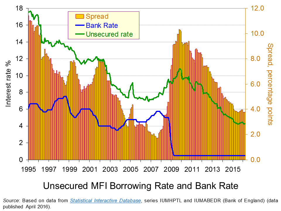
 The chart shows the Bank Rate along with the average unsecured borrowing rate on loans by Monetary Financial Institutions (MFIs) of £10 000. Unlike secured borrowing, which we consider shortly, unsecured borrowing is not secured against property.
As expected, we can see that the unsecured borrowing rate is greater than the Bank Rate. In other words, there is a positive interest-rate differential. However, this differential is seen to vary. It falls sharply in the period up to the financial crisis. In early 2002 it was running at 8 percentage points. By summer 2007 the differential had fallen to only 1.7 percentage points. (Click here to download a PowerPoint of the chart.)
The period from 2002 to 2007 was characterised by consistently robust growth with the UK economy growing by about 2.7 per cent per annum over this period. This may point to economic growth can contributing to an easing of credit conditions as implied by the financial accelerator.
The story from 2008 changes very quickly as the interest-rate differential increases very sharply. In 2009, as the official Bank Rate was cut to 0.5 per cent, the unsecured borrowing rate climbed to close to 10.5 per cent. Consequently, the interest-rate differential rose to 10 percentage points. Inter-bank lending had dried up with banks concerned that banks would default on loans. The increase in interest rates on lending to the non-bank private sector was stark and evidence of a credit market disruption.
The interest-rate differential for unsecured borrowing has steadily declined since its peak at the end of 2009 as the unsecured borrowing rate has fallen. This implies that credit conditions have eased. In March 2016 our interest-rate differential for unsecured borrowing stood at 3.8 percentage points, not dissimilar to levels over the past 12 months. Interestingly, today’s differential on unsecured borrowing is lower than the 6.5 percentage point average over the period from 1997 to 2003, before the differential then went on its pre-crisis fall.
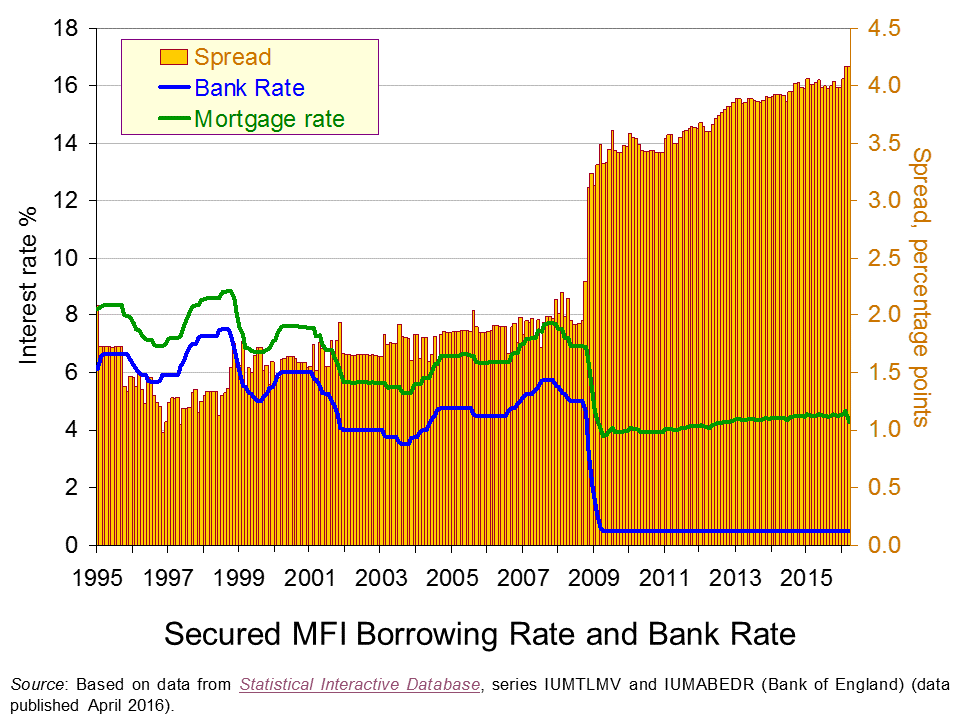
 Our second chart repeats the analysis but this time for mortgages. The representative mortgage rate is the average standard variable mortgage rate.
Unlike that for unsecured borrowing, the interest-rate differential for mortgages is fairly constant up to the financial crisis. The widely report credit easing in the mortgage market appears to have operated more through amounts lent rather than through price, as evidenced by rising mortgage advance-to-income ratios. (Click here to download a PowerPoint of the chart.)
The second chart shows clear evidence of a credit market disruption from 2009. Hence, the markets for secured and unsecured lending saw credit conditions tighten with interest-rate differentials rising markedly. However, it shows that the higher interest-rate differential for secured lending following the credit market disruption remains. So while the differential has fallen sharply for unsecured lending the situation is quite different in the mortgage market. In fact, February and March 2016 saw the mortgage rate spread at 4.17 percentage points which is an historic high.

Our interest rate data show that interest-rate differentials can vary significantly over time. This is important to understand when we are thinking about the relationships between the macroeconomy and the financial system. Significantly, the data suggest that interest rates on different financial instruments can behave differently such that differences emerge in the patterns of spreads over the official Bank Rate.
The evidence on UK mortgage rates suggests that the market remains affected by the financial crisis and the credit market disruption that arose. Although the level of mortgage rates is historically low – which tends to capture many of the headlines – this masks an historically high premium over the official Bank Rate.
Articles
Bank warns EU vote may hit growth as it holds rates BBC News, (14/4/16)
Carney issues a warning as interest rates are held Belfast Telegraph, (15/4/16)
Bank Of England Leaves Interest Rates On Hold Sky News, (14/4/16)
UK banks plan to boost lending to households but not firms – BoE Reuters, (13/4/16)
Mortgage rates reach record lows as threat of Bank Rate rise evaporates Telegraph, Tara Evans (1/4/16)
Data
Bankstats (Monetary and Financial Statistics) – Latest Tables Bank of England
Statistical Interactive Database – interest and exchange rates data Bank of England
Questions
- Why would we expect banks’ borrowing rates to be higher than the official Bank Rate?
- How might banks’ credit criteria change as the macroeconomic environment changes? Explain your answer.
- As well as the macroeconomic environment, what other factors might lead to a change in the interest-rate differential between banks’ borrowing rates and the official Bank Rate?
- How would we expect a credit market disruption to affect the interest-rate differential?
- Explain how the financial accelerator affects the change in the size of the economy following a positive demand shock.
- Explain how the financial accelerator affects the change in the size of the economy following a negative demand shock.
- What is the impact of the financial accelerator of the amplitude of the business cycle?
- How might regulators intervene to minimise the effect of the financial accelerator?
- Why might explain the high interest-rate differential on mortgages that continues to persist following the financial crisis?
- Analyse the ways in which the financial system can stabilise or destabilise economies.
 As John reminds us in his blog A seven year emergency we have now seen the official Bank Rate at 0.5 per cent for the past seven years. Understandably many attribute the financial crisis that led to the easing of monetary policy to the lending practices of commercial banks. Consequently, it is important that we better understand (and monitor) banks’ behaviour. Some argue that these practices are affected by the macroeconomic environment, with credit conditions varying across the business cycle. We consider here what recent patterns in interest rates might tell us about credit conditions.
One way in the macroeconomic environment might affect commercial banks’ lending practices is through the difference between banks’ lending rates and the official Bank Rate. We can think of such interest rate differentials – or spreads – as a credit premium. In other words, the greater are commercial borrowing rates relative to the Bank Rate, the greater the credit premium being demanded by banks. On the other hand, the lower the interest rate on borrowing relative to the Bank Rate, the smaller the credit premium.
Some economists argue that interest-rate differentials will fall when the economy is doing well and increase when the economy is doing less well. This is because the probability of default by borrowers is seen as smaller when the macroeconomic environment improves. If this is the case, it will tend to amplify the business cycle, since economic shocks will have larger affects on economic activity.
Consider a positive demand-side shock, such as a rise in consumer confidence, which lowers the propensity of households to save. As the positive shock causes the economy’s aggregate demand to rise, the economy grows. This growth in economic activity might result in lower borrowing rates offered by commercial banks relative to the official Bank Rate. Since savings rates tend to be close to the official Bank Rate, this also means that the cost of borrowing falls relative to the interest rates on savings. This financial effect further stimulates the demand for credit and, as a consequence, aggregate demand and economic activity. It is an example of what economists called the financial accelerator.
Similarly, the financial accelerator means that negative shocks depress economic activity by more than would otherwise be the case. A fall in consumer confidence, for example, would cause economic activity to fall as aggregate demand weakens. This, in turn, causes banks to raise borrowing rates relative to the Bank Rate and savings rates. This further dampens economic activity.
 The chart shows the Bank Rate along with the average unsecured borrowing rate on loans by Monetary Financial Institutions (MFIs) of £10 000. (Secured borrowing is that which is secured against property.) We use this borrowing rate to capture general trends in commercial borrowing rates.
As expected, we can see that the borrowing rate is greater than the Bank Rate. In other words, there is a positive interest-rate differential. However, this differential is seen to vary. It falls sharply in the period up to the financial crisis. In early 2002 it was running at 8 percentage points. By summer 2007 the differential had fallen to only 1.7 percentage points. (Click here to download a PowerPoint of the chart.)
The period from 2002 to 2007 was characterised by consistently robust growth. The UK economy grew over this period by about 2.7 per cent per annum. This would certainly fit with the story that economic growth may have contributed to an easing of credit conditions which, in turn, helped to induce growth. Regardless, the falling interest-rate differential points to credit conditions easing.
The story from 2008 changes very quickly as the interest-rate differential increases very sharply. In 2009, as the official Bank Rate was cut to 0.5 per cent, the unsecured borrowing rate climbed to close to 10.5 per cent. Consequently, the interest-rate differential rose to 10 percentage points. Inter-bank lending had dried up with banks concerned that banks would default on loans. The increase in interest rates on lending to the non-bank private sector was stark and evidence of a credit market disruption.
The interest-rate differential has steadily declined since its peak at the end of 2009 as the unsecured borrowing rate has fallen. Hence credit conditions have eased. In fact, in February 2016 our indicative interest rate differential stood at 3.8 percentage points, unchanged from its level in January. This is its lowest level since July 2008. Furthermore, today’s differential is lower than the 6.5 percentage point average over the period from 1997 to 2003, before the differential then went on its pre-crisis fall.
Given concerns about the impact of credit cycles on the macroeconomy we can expect the authorities to keep a very keen eye on credit conditions in the months ahead.
Articles
Bank holds UK interest rates at 0.5% BBC News (17/3/16)
UK’s record low interest rates to continue in 2016 The Guardian, Katie Allen (3/3/16)
Big rise in consumer credit in January BBC News, Brian Milligan (29/2/16)
Household debt binge has no end in sight, says OBR The Telegraph, Szu Ping Chan (17/3/16)
Data
Bankstats (Monetary and Financial Statistics) – Latest Tables Bank of England
Statistical Interactive Database – interest and exchange rates data Bank of England
Questions
- Why would we expect banks’ borrowing rates to be higher than the official Bank Rate?
- What factors might lead to a change in the interest-rate differential between banks’ borrowing rates and the official Bank Rate?
- How would we expect a credit market disruption to affect the interest-rate differential?
- Explain how the financial accelerator affects the change in the size of the economy following a positive demand shock.
- Explain how the financial accelerator affects the change in the size of the economy following a negative demand shock.
- What is the impact of the financial accelerator of the amplitude of the business cycle?
- How might banks’ credit criteria change as the macroeconomic environment changes?
- How might regulators intervene to minimise the effect of the financial accelerator?
 In recent times the notion that the financial sytem can be destabilising seems blindingly obvious. And, yet, for some time macroeconomic models of the economy tended to regard the financial system as benevolent. It served our interests. We were the masters; it was our servant. Now of course we accept that credit cycles can be destabilising. Policymakers, especially central banks, follow keenly the latest private-sector credit data. Here we look back at previous patterns in private-sector debt and crucially at what patterns are currently emerging.
First a bit of theory. The idea of credit cycles is not new. But the financial crisis of the late 2000s has helped to reignite analysis and interest. Economists are trying to gain a better understanding of the relationship between flows of credit and the state of the economy and, in particular, why might flows increase as the level of real GDP rises – why might they be endogenous variables in models of the determination of GDP. One possibility is the financial accelerator. This is the idea that as real GDP rises banks perceive lending to be less risky. After all, real incomes will tend to rise and collateral values (against which borrowing can be secured) are likely to be rising too.
Another possibility is growing exuberance as the economy grows. This has gained in popularity as an idea, with economists revisiting the work of Hyman Minsky (1919–96), an American economist. Here success breeds failure as the balance sheets of people and businesses deteriorate as they become increasingly burdened with debt. The balance sheets are said to be congested leading to a point when a deleveraging starts. A balance sheet recession then follows.
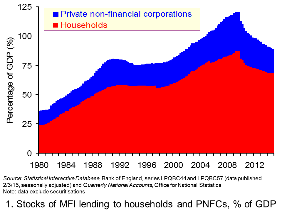
 Now for the data. Consider first the stocks of debt acquired by households and private non-financial corporations from MFIs (Monetary Financial Institutions). The first chart shows debt stocks as a percentage of GDP. It illustrates nicely the phenomenon of financialisation. In essence, this is the increasing importance of MFIs to the economy. At the end of 2014, these two sectors had debt stocks outstanding equivalent to 90 per cent of GDP. In fact, this is down from a peak of 129 per cent in September 2009. (Click here for a PowerPoint of the chart.)
The growth in debt, especially in the 1990s and for much of the 2000s, was through financial innovation. In particular, the bundling of assets, such as mortgages, to form financial instruments which could then be purchased by investors helped to provide financial institutions with further funds for lending. This is the process of securitisation. Some argue that this was part of a super-cycle which works alongside the normal credit cycle, albeit over a much lengthier period. It can be argued that these cycles coincided during the 1990s and for much of the 2000s until financial distress hit. The distress was hastened by central banks raising interest rates to dampen the rising rate of inflation, partly attributable to rising global commodity prices, including oil.
Some refer to 2008 as a Minsky moment. Overstretched balance sheets needed repairing. But, the collective act of repair actually caused financial well-being to worsen as asset prices and aggregate demand fell.
The global response to the events of the financial crisis has been for policy-makers to pay more attention to the aggregate level of credit provision. The Bank of England’s Financial Policy Committee (FPC) has responsibility for monitoring and helping to ensure the soundness of the UK financial system.
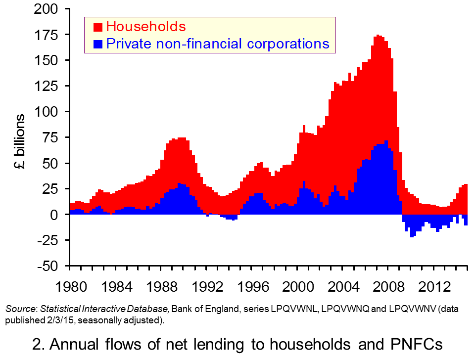
 Undoubtedly, the FPC will have constructed a chart similar to our second chart. (Click here for a PowerPoint of the chart). This chart suggests some caution: the need for casting a ‘Minsky eye’ on lending patterns. Over 2014, the UK household sector undertook net lending (i.e. after deducting repayments) of £30 billion. While nothing like the £100 billion or so in 2007, this does mark something of a step up. Indeed it is almost exactly double the flow in 2013. In the months ahead we will continue to monitor the credit data. You can bet that the FPC will do too!
Articles
Comment: Household debt threatens return to spending Herald Scotland, Bill Jamieson (2/3/15)
Household debt rising at fastest rate for 10yrs moneyfacts.co.uk (10/2/15)
Housing starting to rally after home loan approvals rise in January London Evening Standard, Ben Chu (2/3/15)
Data
Bankstats (Monetary and Financial Statistics) – Latest Tables Bank of England
Statistical Interactive Database Bank of England
Questions
- What is meant by the term the business cycle?
- What does it mean for the determinants of the business cycle to be endogenous? What about if they are exogenous?
- Outline the ways in which the financial system can impact on the spending behaviour of households. Repeat the exercise for businesses.
- How might uncertainty affect spending and saving by households and businesses?
- What does it mean if bank lending is pro-cyclical?
- Why might lending be pro-cyclical?
- How might the differential between borrowing and saving interest rates vary over the business cycle?
- Explain what you understand by net lending to households or firms. How does net lending affect their stock of debt?
 Both the financial and goods markets are heavily influenced by sentiment. And such sentiment tends to be self-reinforcing. If consumers and investors are pessimistic, they will not spend and not invest. The economy declines and this further worsens sentiment and further discourages consumption and investment. Banks become less willing to lend and stock markets fall. The falling stock markets discourage people from buying shares and so share prices fall further. The despondency becomes irrational and greatly exaggerates economic fundamentals.
 But bubbles burst. The question is whether the current global stock market boom, with share prices reaching record levels, represents a bubble. One indicator is the price/earnings (PE) ratio of shares. This is the ratio of share prices to earnings per share. Currently the ratio for the US index, S&P 500, is just over 26. This compares with a mean over the past 147 years of 15.64. The current ratio is the third highest after the peaks of the early 2000s and 2008/9.
 The current level of the Shiller PE ratio is 29.14, the third highest on record, this time after the period running up to the Wall Street crash of 1929 and the dot-com bubble of the late 1990s. The mean Shiller PE ratio over the past 147 years is 16.72.