Tag: correlation

In recent months there has been growing uncertainty across the global economy as to whether the US economy was going to experience a ‘hard’ or ‘soft landing’ in the current business cycle – the repeated sequences of expansion and contraction in economic activity over time. Announcements of macroeconomic indicators have been keenly anticipated for signals about how quickly the US economy is slowing.

Such heightened uncertainty is a common feature of late-cycle slowing economies, but uncertainty now has been exacerbated because it has been a while since developed economies have experienced a business cycle like the current one. The 21st century has been characterised by low inflation, low interest rates and recessions caused by various types of crises – a stock market crisis (2001), a banking crisis (2008) and a global pandemic (2020). In contrast, the current cycle is a throwback to the 20th century. The high inflation and the ensuing increases in interest rates have produced a business cycle which echoes the 1970s. Therefore, few investors have experience of such economic conditions.

The focus for investors during this stage of the cycle is when the slowing economy will reach the minimum. They will also be concerned with the depth of the slowdown: will there still be some growth in income, albeit low; or will the trough be severe enough to produce a recession, and, if so, how deep? Given uncertainty around the length and magnitude of business cycles, this leads to greater risk aversion among investors. This affects reactions to announcements of leading and lagging macroeconomic indicators.

This blog examines what sort of economic conditions we should expect in a late-cycle economy. It analyses the impact this has had on investor behaviour and the ensuing dynamics observed in financial markets in the USA.

The Business Cycle

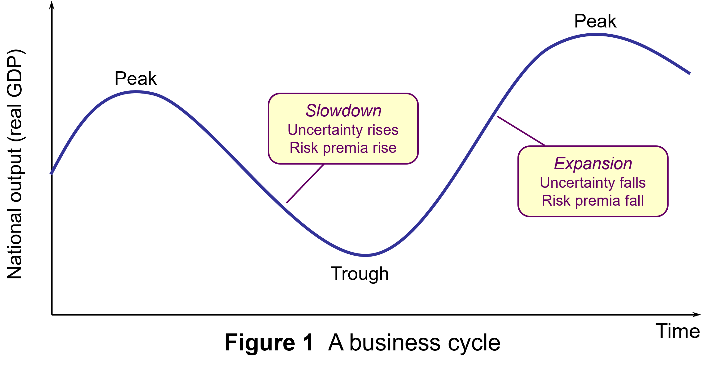
The business cycle refers to repeated sequences of expansion and contraction (or slowdown) in economic activity over time. Figure 1 illustrates a typical cycle. Typically, these sequences include four main stages. In each one there are different effects on consumer and business confidence:

• Expansion: During this stage, the economy experiences growth in GDP, with incomes and consumption spending rising. Business and consumer confidence are high. Unemployment is falling.
• Peak: This is the point at which the economy reaches its maximum output, but growth has ceased (or slowed). At this stage, inflationary pressures peak as the economy presses against potential output. This tends to result in tighter monetary policy (higher interest rates).
• Slowdown: The higher interest rates raise the cost of borrowing and reduce consumption and investment spending. Consumption and incomes both slow or fall. (Figure 1 illustrates the severe case of falling GDP (negative growth) in this stage.) Unemployment starts rising.
• Trough: This is the lowest point of the cycle, where economic activity bottoms out and the economy begins to recover. This can be associated with slow but still rising national income (a soft landing) or national income that has fallen (a hard landing, as shown in Figure 1).

While business cycles are common enough to enable such characterisation of their temporal pattern, their length and magnitude are variable and this produces great uncertainty, particularly when cycles approach peaks and troughs.

As an economy’s cycle approaches a trough, such as US economy’s over the past few months, uncertainty is exacerbated. The high interest rates used to tackle inflation will have increased borrowing costs for businesses and consumers. Access to credit may have become more restricted. Profit margins are reduced, especially for industrial sectors sensitive to the business cycle, reducing expected cash flows.

The combination of these factors can increase the risk of a recession, producing greater volatility in financial markets. This manifests itself in increased risk aversion among investors.

Utility theory suggests that, in general, investors will exhibit loss aversion. This means that they do not like bearing risk, fearing that the return from an investment may be less than expected. In such circumstances, investors need to be compensated for bearing risk. This is normally expressed in terms of expected financial return. To bear more risk, investors require higher levels of return as compensation.

As perceptions of risk change through the business cycle, so this will change the return investors will require from the financial instruments they hold. Perceived higher risk raises the return investors will require as compensation. Conversely, lower perceived risk decreases the return investors expect as compensation.

Investors’ expected rate of return is manifested in the discount rate that they use to value the anticipated cash flows from financial instruments in discounted cash flow (DCF) analysis. Equation 1 is the algebraic expression of the present-value discounted series of cash flows for financial instruments:

 
 
Where:
V = present value
C = anticipated cash flows in each of time periods 1, 2, 3, etc.
r = expected rate of return

For fixed-income debt securities, the cash flow is constant, while for equity securities (shares), expectations regarding cash flows can change.

Slowing economies and risk aversion

In a slowing economy, with great uncertainty about the scale and timing of the bottom of the cycle, investors become more risk averse about the prospects of firms. This this leads to higher risk premia for financial instruments sensitive to a slowdown in economic activity.

This translates into a higher expected return and higher discount rate used in the valuation of these instruments (r in equation 1). This produces decreases in perceived value, decreased demand and decreased prices for these financial instruments. This can be observed in the market dynamics for these instruments.

First, there may be a ‘flight to safety’. Investors attach a higher risk premium to risker financial instruments, such as equities, and seek a ‘safe-haven’ for their wealth. Therefore, we should observe a reorientation from more risky to less risky assets. Demand for equities falls, while demand for safer assets, such as government bonds and gold, rises.

There is some evidence for this behaviour as uncertainty about the US economic outlook has increased. Gold, long seen as a hedge against market decline, is at record highs. US Government bond prices have risen too.

To analyse whether this may be a flight to safety, I analysed the correlation between the daily US government bond price (5-year Treasury Bill) and share prices represented by the two more significant stock market indices in the USA: the S&P 500 and the Nasdaq Composite. I did this for two different time periods. Table 1 shows the results. Panel (a) shows the correlation coefficients for the period between 1 May 2024 and 31 July 2024; Panel (b) shows the correlation coefficients for the period between 1 August 2024 and 9 September 2024.

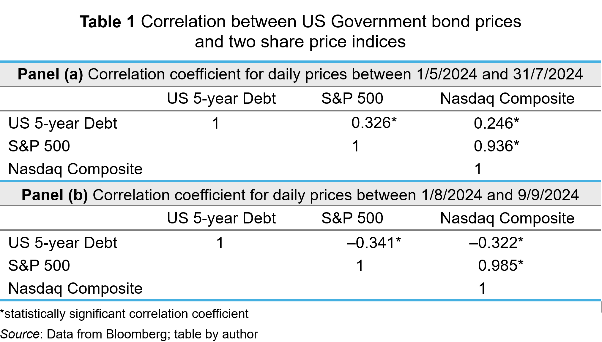
In the period between May and July 2024, the 5-year Treasury Bill and share price indices had significantly positive correlations. When share prices rose, the Treasury Bill’s price rose; when share prices fell, the bill’s price fell. During that period, expectations about falling interest rates dominated valuations and that effected the valuations of all financial instruments in the same way – lower expected interest rates reduce the opportunity cost of holding instruments and reduces the expected rates of return. Hence, the discount rate applied to cash flows is reduced, and present value rises. The opposite happens when macroeconomic indicators suggest that interest rates will stay high (ceteris paribus).

As the summer proceeded, worries about a ‘hard landing’ began to concern investors. A weak jobs report in early August particularly exercised markets, producing a ‘flight to safety’. Greater risk aversion among investors meant that they expect a higher return from equities. This reduced perceived value, reducing demand and price (ceteris paribus). To insulate themselves from higher risk, investors bought safer assets, like government bonds, thereby pushing up their prices. This behaviour was consistent with the significant negative correlation observed between US government debt prices and the S&P 500 and Nasdaq indices in Panel (b).

Another signal of increased risk aversion among investors is ‘sector rotation’ in their equity portfolios. Increased risk aversion among investors will lead them to divest from ‘cyclical’ companies. Such companies are in industrial sectors which are more sensitive to the changing economic conditions across the business cycle – consumer discretionary and communication services sectors, for example. To reduce their exposure to risk, investors will switch to ‘defensive’ sectors – those less sensitive to the business cycle. Examples include consumer staples and utility sectors.

Cyclical sectors will suffer a greater adverse impact on their cash flows and risk in a slowing economy. Consequently, investors expect higher return as compensation. This reduces the value of those shares. Demand for them falls, depressing their price. In contrast, defensive sectors will be valued more. They will see an increase in demand and price. This sector rotation seems to have happened in August (2024). Figure 2 shows the percentage change between 1 August and 9 September 2024 in the S&P 500 index and four sector indices, comprising companies from the communication services, consumer discretionary, consumer staples and utilities sectors.

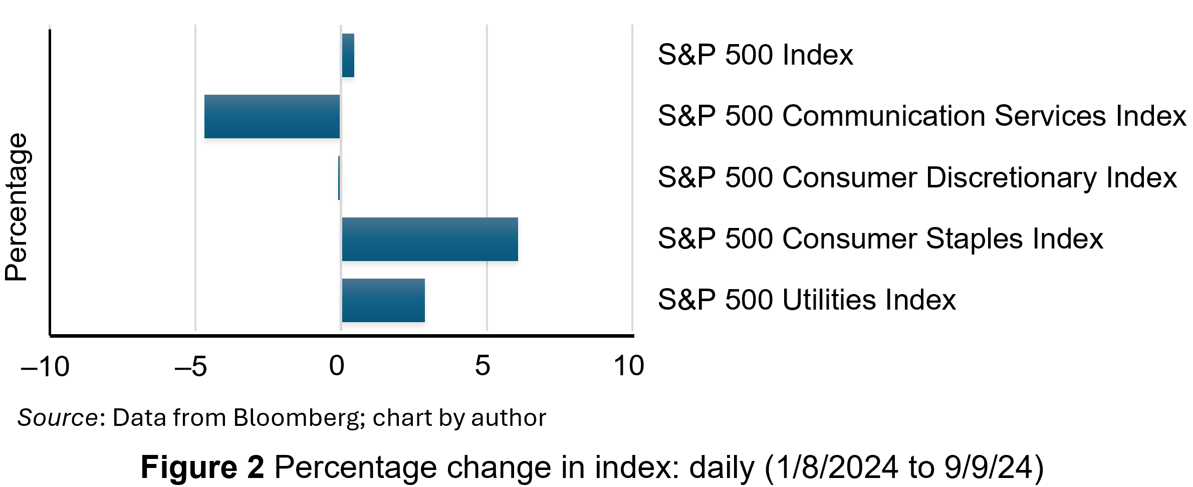
Overall, the S&P 500 index was slightly higher, as shown by the first bar in the chart. However, while the cyclical sectors experienced decreases in their share prices, particularly communication services, the defensive companies experienced large price increases – nearly 3% for utilities and over 6% for consumer staples.

Conclusion

Economies experience repeated sequences of expansion and contraction in economic activity over time. At the moment, the US economy is approaching the end of its current slowing phase. Increased uncertainty is a common feature of late-cycle economies and this manifests itself in heightened risk aversion among investors. This produces certain dynamics which have been observable in US debt and equity markets. This includes a ‘flight to safety’, with investors divesting risky financial instruments in favour of safer ones, such as US government debt securities and gold. Also, investors have been reorientating their equity portfolios away from cyclicals and towards defensive securities.

Articles

• America’s recession signals are flashing red. Don’t believe them

The Economist (22/8/24)

• The most well-known recession indicator stopped flashing red, but now another one is going off

CNN, Elisabeth Buchwald (13/9/24)

• World’s largest economy will still achieve soft landing despite rising unemployment, most analysts believe

Financial Times, Claire Jones, Delphine Strauss and Martha Muir (6/8/24)

• We’re officially on slowdown watch

Financial Times, Robert Armstrong and Aiden Reiter (30/8/24)

• Anatomy of a rout

Financial Times, Robert Armstrong and Aiden Reiter (6/8/24)

• Reasons why investors need to prepare for a US recession

Financial Times, Peter Berezin (5/9/24)

• Business Cycle: What It Is, How to Measure It, and Its 4 Phases

Investopedia, Lakshman Achuthan (6/6/24)

• Risk Averse: What It Means, Investment Choices, and Strategies

Investopedia, James Chen (5/8/24)

Data

• Markets Data

Financial Times

Questions