 The television streaming market is currently attracting considerable attention from policy makers. This follows Warner Bros. accepting Netflix’s offer to buy part of the company for $72bn. To understand how this deal came about and why there is policy concern, we need to go back a few years.
The media and entertainment conglomerate Warner Bros. Discovery (WBD) was created in 2022 when AT&T sold Warner Bros to Discovery.1 However, in June 2025 the company announced that it would split the business into two parts. One would be (a) the studio for TV and movie production, where for example the Harry Potter franchises were made, and (b) the TV streaming business, home to for example the hit TV series Succession. The other, the more traditional and declining TV networks, including channels such as CNN, Discovery and TNT Sports, would form a new company called Discovery Global. David Zaslav, WBD President and Chief Executive stated that:
We are empowering these iconic brands with the sharper focus and strategic flexibility they need to compete most effectively in today’s evolving media landscape.2
Shortly afterwards, rival media and entertainment conglomerate, Paramount Skydance, made a series of bids to purchase the entire WBD business. But these were rejected by the WBD board. Despite this, in October 2025 WBD made public that it was open to a sale and had received unsolicited interest from several companies. It was believed that this included offers from Comcast and Netflix.
Recent developments
 In December 2025, Netflix announced that it had agreed a deal with WBD to buy its studio and streaming service business, including its back catalogue of shows. The deal is planned to be put to WBD shareholders in the next few months.3 Netflix has over 300m subscribers across the globe and streams popular shows, such as Stranger Things and Squid Games.
Despite this accepted offer, Paramount has subsequently pursued a hostile takeover of WBD by going straight to its shareholders. In addition, Paramount launched a lawsuit to get further information on how Netflix was chosen as the buyer and to provide WBD shareholders with information on the value of the TV network business that WBD was selling. This, however, was quickly thrown out of the courts.
Over time, Netflix and Paramount have tinkered with their bids to make them more attractive to WBD. Whilst Paramount’s bid was all cash, originally Netflix was offering a mixture of cash and shares. However, in January, it switched this to an all-cash offer. In February, Paramount made clear that if WBD instead accepted its offer, it would pay the $2.8bn termination fee that would be owed to Netflix.4 Furthermore, from early 2027 Paramount would pay WBD shareholders payments of $650m per quarter, known as ticking fees, if combining WBD and Paramount faced regulatory delay.
In mid-February 2026, it emerged that, following a waiver from Netflix, WBD had reopened talks with Paramount. Paramount was given a week to make its offer. Then, under the agreed deal, Netflix would have the right to adjust its bid. This is an attempt by WBD to end the hostile bidding war Paramount is pursuing and to provide clarity for its shareholders. WBD has reiterated that it will:
continue to recommend and remain fully committed to our transaction with Netflix. [However], we welcome the opportunity to engage with you and expeditiously determine whether Paramount Skydance can deliver an actionable, binding proposal that provides superior value.5
The insertion of the ticking fees by Paramount is in response to the substantial attention competition authorities across the globe are paying to the acquisition of WBD. The deal is being investigated by the US Department of Justice and, in early February, Netflix was questioned by the US Senate Antitrust Sub-committee. During this hearing, one of the Senators expressed his anger with the country’s competition laws and raised concerns that the deal would result in Netflix getting:
more power over consumers and leaving fewer alternatives and streaming platforms.6
While Paramount did not attend this hearing, it is believed that it has raised concerns about the Netflix-WBD deal to regulators. Netflix co-CEO, Ted Sarandos, has also met with Donald Trump to discuss the deal. However, Trump subsequently stated that the deal ‘could be a problem’.7
The EU and UK markets
 Furthermore, whilst all the companies involved are American, both the mergers with Netflix and Paramount are being investigated by the European Commission as markets in Europe would be affected.
In the UK, a group of politicians and former policymakers, have written to the Competition and Markets Authority urging it to conduct a full investigation of the Netflix-WBD merger. The letter argues that the merger could have:
damaging consequences for consumers, the UK’s world-leading creative industries and the UK cinema industry.
and that:
At a time when the British consumer can ill-afford more price increases, Netflix would possess an unprecedented ability to raise prices to access television and films.8
 The letter comes at a time when pressure is being placed on the CMA to adopt a generally more business-friendly approach.
The impact of the merger on the UK market is particularly complicated since Warner Bros.’ streaming service, HBO Max, is only due to launch in the UK in March 2026. This is still the plan, with WBD’s head of global streaming, Jean-Briac Perette acknowledging that:
We are likely the last scaled global streamer to come to market. We’ve tried to learn from the rest. We’re a complementary and distinct service to the more volume-driven or basic cable-like streamers in the market. More is not better. Better is better.9
An alternative route to regulatory approval
An easier route to regulatory approval may well be instrumental in allowing Netflix or Paramount to win the battle for WBD. Netflix stresses that the deal will create economic growth and jobs. Netflix’s Sarandos highlighted that:
This is not a typical media merger where you end up with what’s called the Noah’s Ark problem — two of everything. We are buying a company that has assets that we do not, and we will keep investing in those.10
The problem of economic power
In contrast, critics argue that either of the deals would create a new company with too much power. However, given the nature of the firms involved, the competition issues will be fundamentally different between the two deals.
 The Paramount deal would primarily reduce the number of studios in the market. This could provide the new merged studio with more bargaining power over distributors, advertisers and creators. Ultimately, this could negatively impact on the final product that consumers watch in the cinema and on television.
The Netflix deal on the other hand would impact directly on the streaming market. In the USA, 80% of consumers have both Netflix and HBO Max.11 After the merger, consumers would have less choice of competing services and Netflix-HBO Max combined may well have an incentive to raise its subscription prices.
In the UK, there are currently three leading streaming services: Netflix, Amazon Prime and Disney+, each with around 23% of the market.12 The merger with WBD could allow Netflix to become the clear market leader.
Concerns about YouTube
When examining streaming markets in all countries, an important factor will be whether to include YouTube in the market. Netflix certainly argues that it is a key competitor, at the hearing Sarandos stated that:
we are competing for the same content, we are competing for the same viewers, we are competing often for the same ad dollars. YouTube is not just cat videos anymore. YouTube is TV.13
If YouTube is included, in the USA it would be the market leader with 13%, ahead of Netflix on 9%. However, the competition authorities may conclude that YouTube’s product and business model is sufficiently different and so not include it in the streaming market.14
The issue of cinemas
 A second concern in the Netflix deal will be the Warner Bros.’ studio content that Netflix would own. The merged business may have an incentive to discontinue, raise the price or reduce the quality of the studio output that it supplies to cinemas. Thus, the competition authorities’ investigations will also pay close attention to the impact on the cinema market.
In line with these arguments, the Hollywood screenwriters’ union, the Writers Guild of America, has indicated that the Netflix-WMD deal should be stopped and filmmakers are clearly concerned about Netflix prioritising streaming.15
The competition authorities may well consider imposing remedies before they are willing to allow either deal to go ahead. With this in mind, it is interesting that Netflix has already made clear that it will continue the 45-day exclusive window that Warner Bros. provides cinemas to show its films.
It will be fascinating to see how the competing bids play out and how the competition regulators view them.
* * *
This post has been updated in a Postscript, following a further bid from Paramount that was not matched by Netflix.
References
- AT&T agrees deal to combine WarnerMedia with Discovery
The Guardian, Mark Sweney (16/5/21)
- HBO and CNN owner to split streaming and cable businesses
BBC News, Adam Hancock (10/6/25)
- Netflix’s co-CEO went to an antitrust hearing and a culture war broke out
NBC News, Saba Hamedy (3/2/26)
- Warner Bros gives Paramount seven days to make ‘best and final’ offer
The Guardian, Mark Sweney (17/2/26)
- ibid.
- NBC News, op. cit.
- Trump says $72bn Netflix-Warner Bros deal ‘could be a problem’
BBC News, Osmond Chia (8/12/25)
- UK politicians call for competition review of Netflix bid for Warner Bros
Financial Times (26/1/26)
- Warner streaming boss defends HBO Max UK launch ahead of Netflix takeover
Financial Times (9/2/26)
- NBC News, op. cit.
- Netflix and Warner Bros struggle to defend merger
BBC News, Danielle Kaye (3/2/26)
- Netflix, Disney+, Prime: Streaming platform market share report UK 2025
InsiderMedia, Jennifer O’Keeffe (2/12/25)
- BBC News, Danielle Kaye op. cit.
- Paramount sweetens Warner Bros bid with offer to pay Netflix break-up cost, other fees
Reuters, Harshita Mary Varghese and Aditya Soni (11/2/26)
- In a takeover of Warner Bros., Netflix makes a play for 21st century Hollywood’s throne
NBC News, Daniel Arkin (5/12/25)
Articles
Questions
- What are the similarities and differences between Netflix’ and YouTube’s business models? How close substitutes do you think they are?
- Do you think cinemas are a closer or more distant substitute to Netflix than YouTube?
- Which deal do you think raises the most competition concerns? What might be a possible remedy that could alleviate these concerns?
 At the fourth anniversary of Russia’s invasion of Ukraine, we look at the effect of the war on the Russian economy. Two years ago, in the blog The Russian economy after two years of war, we argued that the Russian economy had seemingly weathered the war successfully.
Unlike Ukraine, very little of its infrastructure had been destroyed; it had started the war with a current account balance of payments surplus, a budget surplus and a low general government debt-to-GDP ratio; it had achieved a lot of success in diverting its exports, including oil, away from countries imposing sanctions to countries such as China and India; it was the same with imports, with China especially becoming a major suppliers of machinery, components and vehicles; it has a strong central bank, which engenders a high level of confidence in managing inflation; the military expenditure provided a Keynesian boost to the economy, with production and employment rising.
The situation today
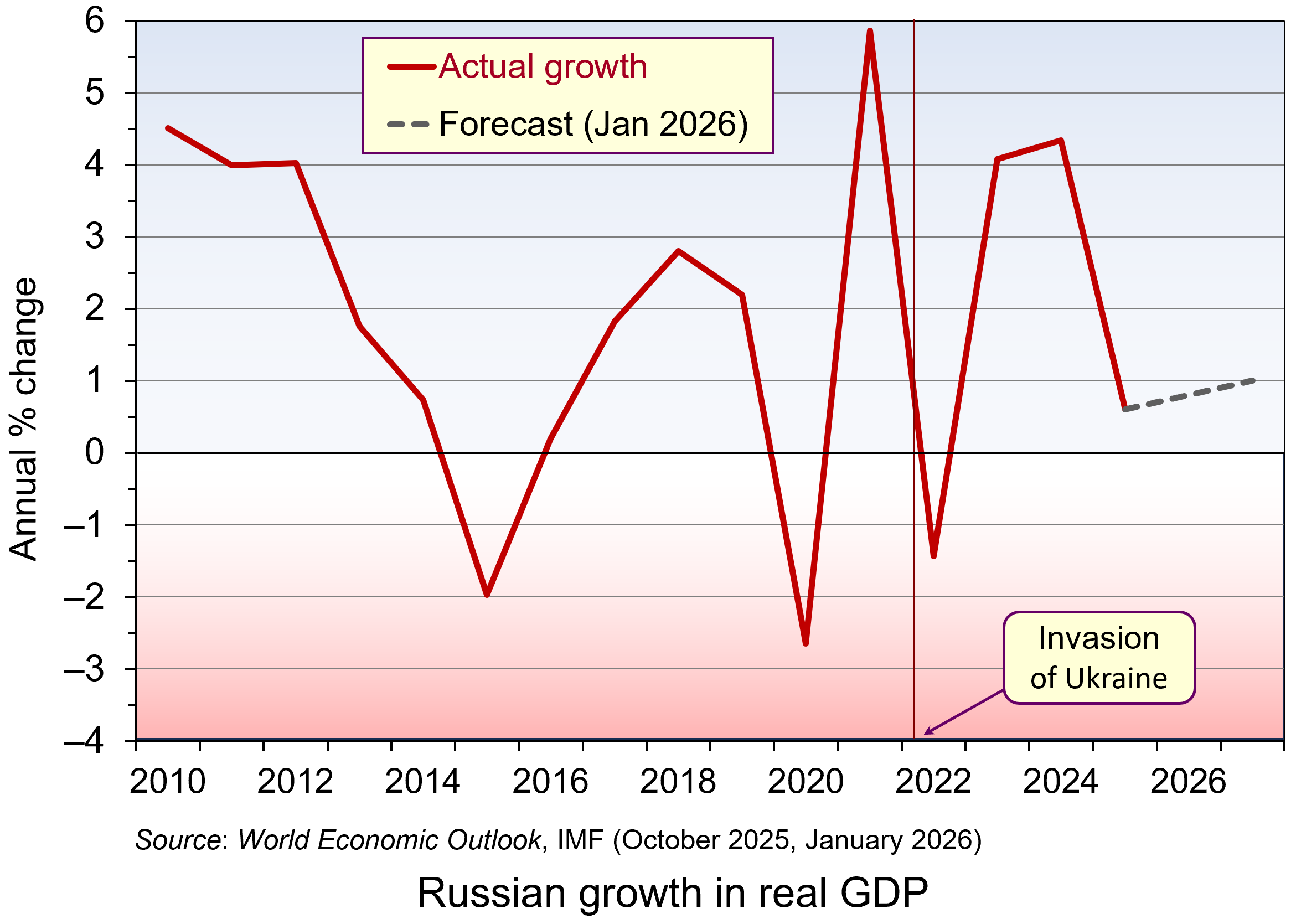 But two years further on, the Russian economy is looking a lot weaker and on the verge of recession. GDP growth fell to 0.6 per cent in 2025 and is forecast to be no more than 1 per cent for the next two years. (Click here for a PowerPoint of the chart.) And despite growth still being positive (just), this is largely because of the growth in military expenditure. Retail and wholesale trade fell by 1.1% in 2025, reflecting supply chain problems and high inflation dampening consumer demand.
With labour being diverted into the armaments and allied industries or into the armed forces, this has led to labour shortages. This has been compounded by the emigration of up to 1 million people by 2025 – often young, educated and skilled professionals.
 Official CPI inflation averaged 8.7 per cent in 2025, although the prices of food and other consumer essentials rose by more, especially in recent months. At the beginning of 2026, supermarket prices rose by 2.3% in just one month, made worse by a rise in VAT from 20% to 22%. The central bank has responded to the high inflation with high interest rates, which averaged 19.2% in 2025, giving a real rate of 10.5%. With such a high real rate, the response of households has been to save. This has masked the constraints on production, or imports, of consumer goods. Savings have also been boosted by large payments to soldiers and bereaved families, with the money saved by the recipients being used in part to fund future such payments. So far there has been trust in the banking system, but if that trust waned and people starting making large withdrawals of savings, it could be seriously destabilising.
Whilst the high real interest rates have helped to mask shortages of consumer goods, they have had a seriously dampening effect on investment by domestic companies. Gross capital formation fell by 3% in 2025, not helped by an increase in the corporation tax from 20% to 25%. At the same time, foreign direct investment remains subdued due to high perceived risks. The lack of investment, plus the labour shortages, will have profound effects on the supply side of the economy, with potential output in the non-military sector likely to decline over the medium term.
 The balance of payments and government finances are turning less favourable. The balance of trade surplus has declined from US$173bn in 2021 to US$67bn in 2025. This could decline further, or even become a deficit, if oil prices continue to be weak, if Western sanctions are tightened (such as stopping the flow of Russian oil exports in the ‘shadow’ fleet of tankers) or if major importing countries stop buying Russian oil. Indian refiners have announced that they are not taking Russian crude in March/April as India seeks to finalise a trade deal with the USA.
The budget balance has moved from a small surplus of 0.8% of GDP in 2021 to a deficit of 2.9% in 2025. Although the government debt-to-GDP ratio remains low by international standards at 23.1% of GDP in 2025, this was up from 16.5% in 2021 and is set to rise further as budget deficits deepen. Nevertheless, as long as the saving rate remains high, the debt can be serviced by domestic bond purchase.
Russia’s economy is definitely weakening and labour shortages and low investment will create major problems for the future. But whether this deterioration will be enough to change Russia’s stance on the war in Ukraine remains to be seen.
Articles
- The Russian economy is finally stagnating. What does it mean for the war – and for Putin?
The Guardian, Alex Clark (6/2/26)
- Exclusive: Russia’s budget deficit may almost triple this year as oil revenues decline
Reuters (4/2/26)
- Russia’s war economy is not collapsing, but neither is it stable
The Conversation, Yerzhan Tokbolat (17/12/25)
- Food prices are surging in Russia. Is the war hitting Russians in the pocket?
BBC News, Olga Shamina, Yaroslava Kiryukhina and Sergei Kagermazov (18/2/26)
- [Russian] GDP data — what it reveals, what it conceals
The Bell, Denis Kasyanchuk (18/2/26)
 What to Expect From the Russian Economy in 2026
Carnegie Endowment for International Peace, Alexandra Prokopenko and Alexander Gabuev (12/2/26)
- Indian refiners avoid Russian oil in push for US trade deal
Reuters, Nidhi Verma (8/2/26)
- What Breaks First – Russia’s Economy or Its War?
Visegrad Insight, Tomasz Kasprowicz (3/2/26)
Videos
Reports
Data
Questions
- What constraints are there currently on the supply side of the Russian economy?
- Some economists have argued that the economic effects of a stalemate in the Ukraine war would suit the Russian leadership more than peace or victory. Why might this be so?
- Under what circumstances might a deep recession in Russia be more likely than stagnation?
- In what ways does Russia’s current financial system resemble a pyramid scheme?
- What cannot a Keynesian boost contunue to support the Russian economy indefinitely?
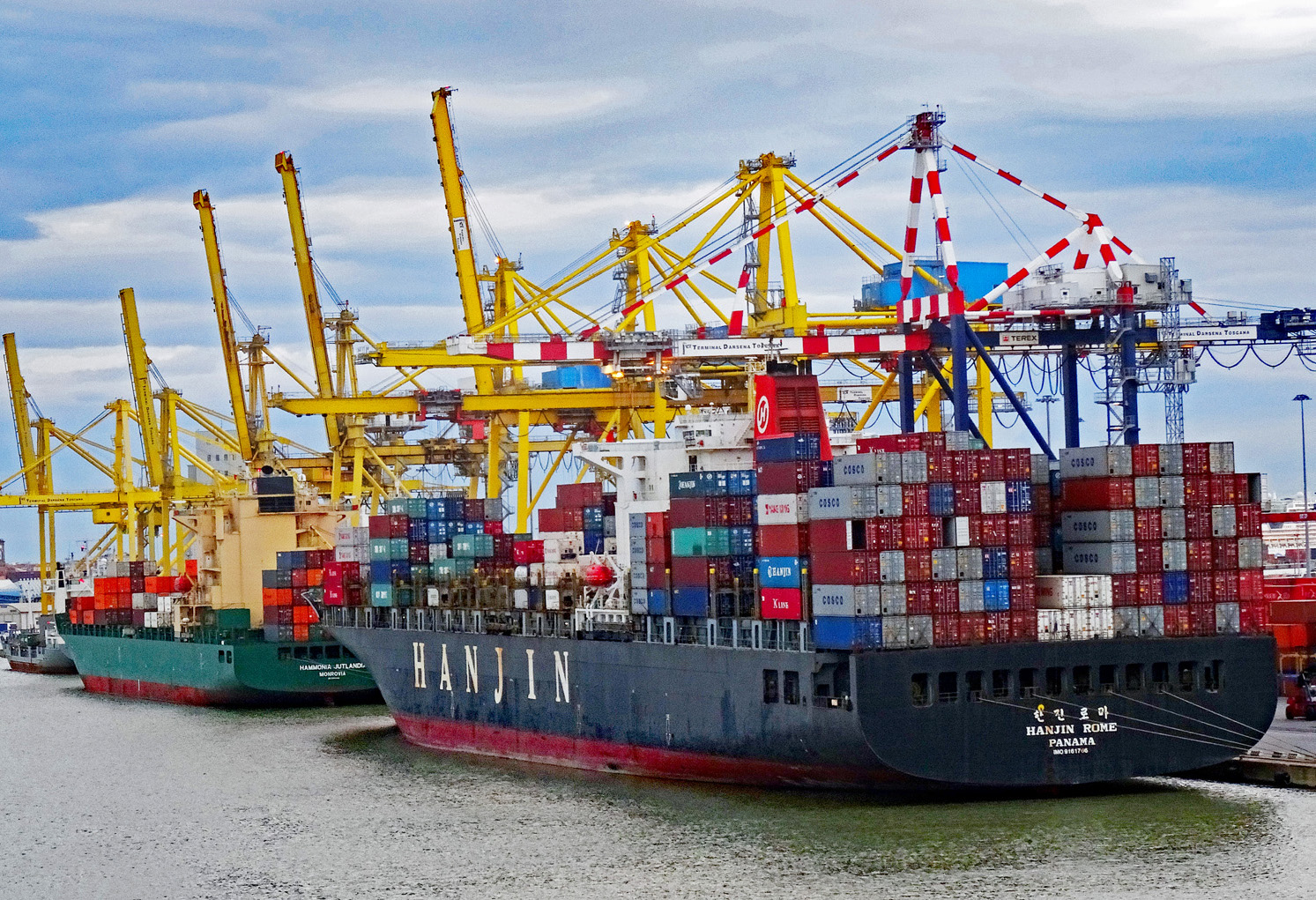 Three recent reports (see links below) have suggested that US consumers and businesses pay most of the tariffs imposed by the second Trump administration. The percentage varies from around 86% to 96%. US customs revenue surged by approximately $200 billion in 2025, but this was a tax paid almost entirely by US consumers and businesses. Foreign suppliers largely maintained their (pre-tariff) prices. They took a hit in terms of reduced volumes rather than reduced pre-tariff prices.
The incidence of a tariff between consumers, domestic importers and overseas producers will depend on price elasticities of demand and supply. The following diagram shows a product where the importing country is large enough to have a degree of market power, which will normally be the case with the USA. The greater its buying power, the flatter will be its demand curve, showing that the foreign supplier will have little influence on the price. With no tariff, the equilibrium price paid by importers will be at point a, where demand equals supply. Q1 would be imported at a price of P1.
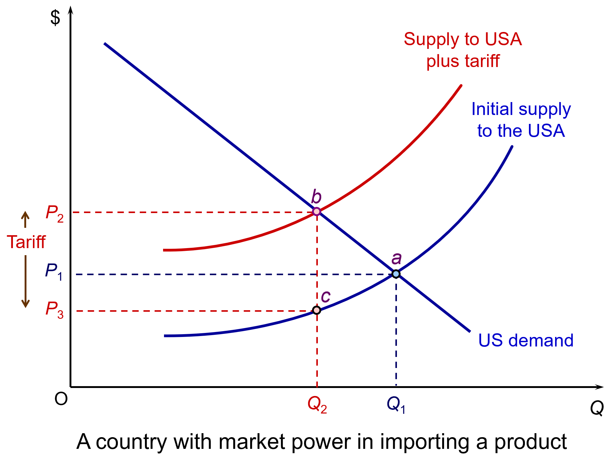 Imposition of a tariff will shift the supply curve upwards by the amount of the tariff. The new equilibrium price paid by importers will be at point b, where the new supply curve crosses the demand curve. Importers thus now pay a post-tariff price of P2: an effective rise in price of P2 minus P1. Foreign exporters receive P3, which is what they are paid by importers after the tariff has been paid.
The consumer price will be above P2 as that includes a mark-up by US businesses on top of the price they pay to import the product. Importers may bear some of the increase in price and not pass the full amount onto consumers, depending on competition and their ability to absorb cost increases.
President Trump argued that there would be very little rise in price from the tariffs and that overseas suppliers would bear the brunt of the tariffs. Indeed, recently he has argued that this must be the case as US inflation has been falling. In response, critics maintain that the rate of inflation would have fallen more without the tariffs and that current prices would be lower than they are. Also, if US importing firms or retailers bear some of the increased cost, even though this helps to dampen the price rise, their lower profits could damage investment and employment.

The Reports
The first report is from the New York Fed (one of the regional branches of the Federal Reserve Bank). It examines the effect of tariffs imposed in 2025, over three periods: (i) January to August, (ii) September to October, and (iii) November. In the first period, 94% of the tariffs were paid by US importers and 6% by foreign exports; in the second period, the figures were 92% and 8% and in the third period, 86% and 14%.
The second report is The Budget and Economic Outlook: 2026 to 2036 from the Congressional Budget Office. Box 2-1 notes that, as of November 2025, ‘the effective tariff rate was about 13 percentage points higher than the roughly 2 percent rate on imports in 2024’. Its analysis suggests that 95% of the tariffs will be borne by importers. Of these higher import prices, 30% will be borne by US businesses, largely through reduced profit margins, and 70% by consumers through higher prices. This will also allow many businesses which produce goods that compete with foreign imports to ‘increase their prices because of the decline in competition from abroad and the increased demand for tariff-free domestic goods’.
The third report is from the Kiel Insitut. In its Policy Brief, Americaʼs Own Goal: Who Pays the Tariffs?, it finds that US importers and consumers bear 96% of the cost of the 2025 tariffs, with foreign exporters absorbing only about 4%. It bases it findings on shipment-level data covering over 25 million transactions valued at nearly $4 trillion. This also shows that exports to the USA declined as foreign exporters preferred to reduce volumes rather than absorbing the tariffs.
The tariffs raised some $200 billion in 2025, around 3.8% of Federal tax receipts. But, as we have seen, this was paid largely by US consumers and business. It goes some way to offsetting the annual cut in tax revenues of around $450 to $520 billion per year from the tax cuts, largely to the better off, in Trump’s ‘One Big Beautiful Bill’.
Reports
Aricles
- NY Fed report says Americans pay for almost all of Trump’s tariffs
Reuters, Michael S. Derby (12/2/25)
- A year in, it’s official: Americans, not foreigners, are paying for Trump’s tariffs
CNN, Allison Morrow (12/2/26)
- Costs from Trump’s tariffs paid mainly by US firms and consumers, NY Fed says
BBC News, Kali Hays (13/2/26)
- Consumers and businesses paid nearly 90% of Trump tariffs in 2025, new analysis found
CBS News, Megan Cerullo (12/2/26)
- New Studies Challenge Who Really Pays for Tariffs
Investopedia, Diccon Hyatt (12/2/26)
- Trump Tariffs: Tracking the Economic Impact of the Trump Trade War
Tax Foundation, Erica York and Alex Durante (6/2/26)
- Who Is Paying the Trump Tariffs?
Paul Krugman (15/2/26)
Questions
- Summarise the findings of the three reports (but just Box 2-1 of the Congressional Budget Office one).
- Assess the argument that protectionism leads to inefficiency in the protected industries.
- Under what circumstances would exporters to the USA absorb a high percentage of tariff increases? Consider questions of elasticity.
- Can tariffs ever be justified on efficiency grounds?
- Can tariffs be justified as a bargaining ploy? Can they be used as a means of achieving freer and fairer trade?
- Read the blog, President Reagan on tariffs and summarise President Reagan’s arguments. Are they still relevant today?
- Consider the arguments for and against the EU raising tariffs on US goods.
 Have you noticed that many products in the supermarket seem to be getting smaller or are poorer quality, or that special offers are not as special as they used to be? When you ring customer services, does it seem that you have to wait longer than you used to? Do you now have to pay for extras that used to be free? These are all ways that producers try to pass on cost increases to consumers without rising prices. There are three broad ways in which producers try to hide inflation.
The first is called ‘shrinkflation’. It is defined as having less product in the same package or a smaller package for the same price. For example, reducing the number of chocolates in a tub, reducing the size of a can of beans, jar of coffee or block of butter, reducing the number of sheets in a toilet roll, or the length of a ride in a fairground or portion sizes in a restaurant or takeaway. A 2023 YouGov poll revealed that 75% of UK adults are either ‘very’ or ‘fairly’ concerned about shrinkflation. A similar poll in 2025 showed that this figure had increased to 80%. The product category with the greatest concerns was snack foods (e.g. crisps, confectionery items, nuts, etc.).1
The second form of hidden inflation is called ‘skimpflation’. This is defined as decreasing the quality of a product or service without lowering the price. Examples include cheaper ingredients in food or confectionery, such as using palm oil instead of butter, or reducing the cocoa content in chocolate or the meat content in sausages and pies, or package holidays reducing the quality of meals, or customer service centres or shops reducing the number of staff so that people have to wait longer on the phone or to be served.
The third is called ‘sneakflation’. This is similar to skimpflation but normally refers to reducing what you get when you pay for a service, such as a flight, by now charging for extras, such as luggage or food. Sometimes shrinkflation or skimpflation are seen as subsets of sneakflation.
 These practices have had a lot of publicity in recent months, with consumers complaining that they are getting less for their money. Many people see them as a sneaky way of passing on cost increases without raising the price. But the changes are often subtle and difficult for shoppers to spot when they are buying an item. Skimpflation especially is difficult to observe at the time of purchase. It’s only when people consume the product that they think that it doesn’t seem as good as it used to be. Even shrinkflation can be hard to spot if the package size remains the same but there is less in it, such as fewer biscuits in a tin or fewer crisps in a packet. People would have to check the weight or volume, while also knowing what it used to be.
If firms are legitimately passing on costs and are up-front about what they are doing, then most consumers would probably understand it even if they did not like it. It’s when firms do it sneakily that many consumers get upset. Also, firms may do it to increase profit margins – in other words, by reducing the size or quality beyond what is necessary to cover the cost increase.
Does the official rate of inflation take such practices into account?
 The answer is that some of the practices are taken into account – especially shrinkflation. The Office for National Statistics (ONS) accounts for shrinkflation by monitoring price changes per unit of weight or volume, rather than just the price. Data collectors track the weight, volume or count of item. When a product’s size is reduced, the ONS records this as a price increase in CPI or CPIH inflation statistics. This is known as a ‘quality adjustment’ process and allows the ONS to isolate price changes from product size changes. As CPI data from the ONS is used by the Bank of England in monitoring its 2% inflation target, it too is incorporating shrinkflation.
ONS quality adjustments are also applied to non-market public services, such as healthcare, education and policing to measure changes in service quality rather than just volume. This allows a more accurate measurement of productivity as it focuses on outcomes and user experience per pound spent rather than just focusing on costs.
Skimpflation is more difficult to monitor. The quality adjustment process may miss some quality changes and hence some skimpflation goes unrecorded. This means that the headline inflation rate might understate the true decline in purchasing power felt by consumers.
How extensive is hidden inflation?
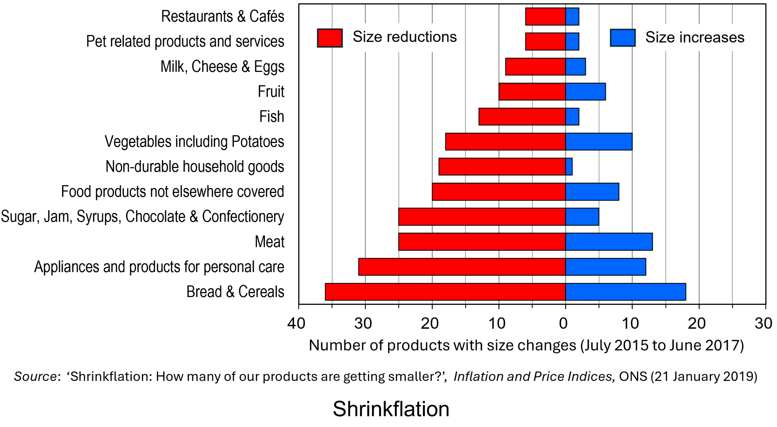
Despite public perception, shrinkflation has a relatively small impact on the headline CPI and CPIH inflation rate in the UK because it is largely confined to certain sectors, such as bread and cereals, personal care products, meat products, and sugar, jams, syrups, chocolate & confectionery. Nevertheless, in these sectors it is particularly prevalent, especially in the packaged foodstuffs and confectionery sector. The latest research by the ONS in 2019 covered the period June 2015 to June 2017 and is shown in the following figure.2
According to research in the USA by Capital One Shopping, some major brands reduced product sizes by over 30% in 2025 without reducing prices, with shrinkflation averaging 14.8% among selected national grocery brands.3 Shrinkflation had been observed by 74% of Americans at their grocery store. Of these, 81% took some kind of action as a result, with 48% abandoning a brand. Nevertheless, across all products, shrinkflation accounts for quite a small percentage of any overall price rises.
A US Government Accountability Office (GAO) report found that shrinkflation accounted for less than 1/10 of a percentage point of the 34.5% increase in overall consumer prices from 2019 to 2024.4 The reason is that the items that were downsized comprised a small percentage of goods and services. Indeed, many goods and services, such as housing, cannot be downsized in the same way that household products can.
Nevertheless, with consumer budgets being squeezed by the inflation that followed the pandemic and the Russian invasion of Ukraine, hidden inflation has become more prevalent in many countries and an increasing concern of consumers.
References
- Shrinkflation concern rises in 2025, but fewer Britons are changing shopping habits
YouGov (15/8/25)
- Shrinkflation: How many of our products are getting smaller?
Office for National Statistics (21/1/19)
- Shrinkflation Statistics
Capital One Shopping (30/12/25)
- What is “Shrinkflation,” And How Has It Affected Grocery Store Items Recently?
U.S. Government Accountability Office (12/8/25)
Videos
Articles
- Shrinkflation: How many of our products are getting smaller?
Office for National Statistics (21/1/19)
- Shrinkflation: Inflation hiding in plain sight
Britannica Money, Doug Ashburn (21/7/25)
- Shrinkflation: the brands charging you more for less
Which?, Ellie Simmonds (28/10/25)
- 7 Surprising Ways Inflation Is Still Rising Even as Prices Slow This Year
SavingAdvice.com, Teri Monroe (3/2/26)
- 22 Real-Life Examples Of Shrinkflation That People Have Spotted In The Last Few Weeks That Are Honestly Infuriating
BuzzFeed, Megan Liscomb (10/12/25)
- Shrinkflation: smaller products hurt some households more than others – and can be bad for business
The Conversation, Erhan Kilincarslan (14/1/26)
- Shoppers brand the UK “a disgrace” as Cadbury Mini Egg prices rise by 105% on pre-pandemic levels
Food Manufacture, Thomas West (6/1/26)
- This article is more than 3 months old Shrinkflation hits everyday staples, piling more pressure on households
The Guardian, Sarah Marsh and Sarah Butler (28/12/25)
- Shrinkflation isn’t slowing down — It’s just getting harder to spot
ConsumerAffairs, Kyle James (13/1/26)
- Shrinkflation – are brands and supermarkets required to inform consumers if a product has been reduced in size or quantity but the packaging looks the same?
CMS Law-Now, Loïc de Hults and Tom Heremans (25/9/25)
- Study reveals shrinking package sizes hide significant food inflation
Phys.org, Aaron Kupec (28/1/26)
Journal Article
Questions
- If shrinkflation, when included in CPI statistics, accounts for such a small percentage of inflation, why are people so concerned about it?
- From a company’s perspective, is it a good idea to engage in (a) shrinkflation; (b) skimpflation?
- Go round you local supermarket and identify examples of shrinkflation and skimpflation.
- How are various EU countries attempting to inform consumers of shrinkflation?
- Why is skimpflation often harder to detect than shrinkflation?
- Give some other examples of sneakflation in the provision of services.
- How could behavioural economists help firms decide whether or how to engage in shrinkflation or skimpflation?
 Precious metals, such as gold, silver and platinum, are seen as safe havens by investors in uncertain times. With the on-off nature of Donald Trump’s tariffs, with ongoing wars, such as the war in Ukraine, and with threats of US action in Iran, with inflation slow to fall and pressure by the Trump administration on the Federal Reserve to make precipitant cuts in interest rates, investors have flocked to precious metals.
Precious metals peaked in late January 2026. Compared with just four months earlier, gold was up by 48%, platinum by 76% and silver by a massive 162%. Silver and platinum were also boosted by their industrial uses. Silver has excellent conductive properties and is used for electronics, AI, solar energy (photovoltaic cells), chemical catalysts and medical equipment. Over 50% of its consumption is for industrial purposes. Platinum is used as a catalyst in catalytic converters to reduce exhaust emissions, in medical devices, chemical processing, oil refining, electronics and glass manufacturing.
The rise was fuelled by speculation, which gathered momentum in December and January. But then the prices of all three metals fell dramatically on Friday 30 January and a bit more on 2 February. Despite a moderate bounce back on 3 February, the prices then fell again and by the end of 5 February, gold had fallen by 15%, platinum by 30% and silver by a massive 42% from the peak.
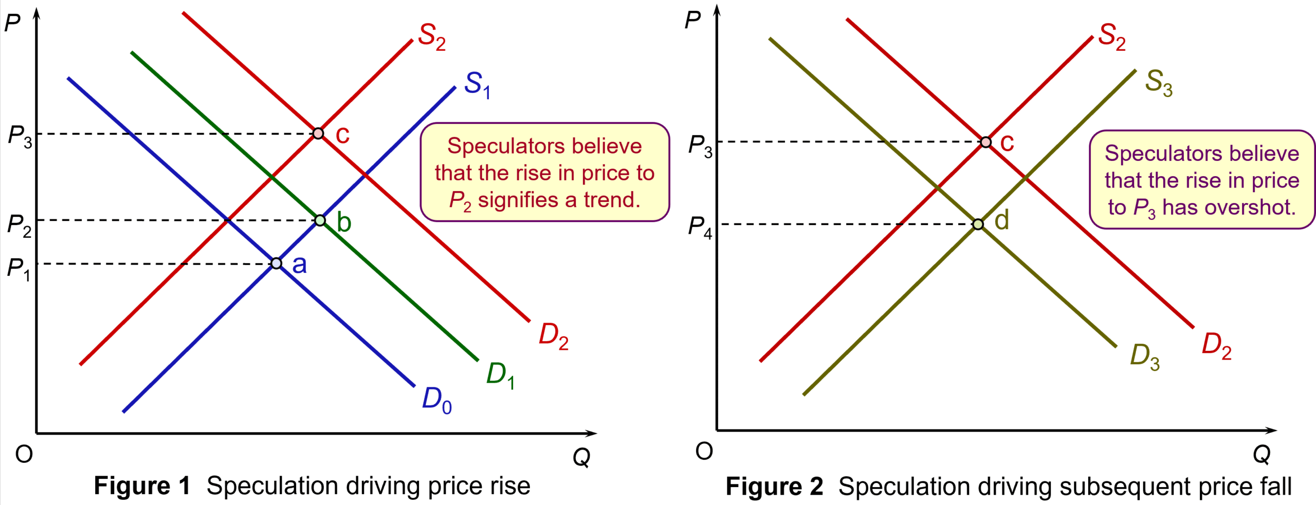
Figure 1 illustrates the effect of speculation on the rise in price of a precious metal, such as silver. Assume that demand rises from D0 to D1 for the reasons given above. Equilibrium moves from point a to point b and the price rises from P1 to P2. Seeing the price rising, holders of the metal wait until the price rises further before selling. Supply shifts from S1 to S2. Potential purchasers of the metal, anticipating a further rise in price, buy now before the price does rise. Demand shifts from D1 to D2. As a result, equilibrium moves from point b to point c and price rises to P3.
Figure 2 illustrates the effect of speculation on the subsequent fall in prices triggered by a belief that price will fall. Speculative selling shifts the supply curve from S2 to S3. Potential demanders hold back and the demand curve shifts from D2 to D3. Equilibrium moves to point d and price falls from P3 to P4. (Click here for a PowerPoint of the two figures.)
But why did prices fall so dramatically? The first reason was that analysts were beginning to argue that the exuberance of investors had led the price of all three metals to overshoot the fundamental balance of supply and demand. Once a tipping point arrived, people sold quickly to lock in the gains they had made over previous weeks. This profit taking caused prices to plummet as speculation of further falls drove prices lower.
 So what was the tipping point? This was the appointment by Donald Trump of Kevin Warsh as the new Chair of the Federal Reserve to take over from Jerome Powell when his tenure comes to an end in May this year.
It was expected that Trump would appoint someone much more willing to cut interest rates and this worried investors, who feared that inflation would rise again. This uncertainty drove demand for precious metals, which are seen as a safe haven. But Kevin Walsh is viewed as hawkish on monetary policy and less likely to slash interest rates than other possible choices for Chair. This triggered the fall in precious metal prices.
But the main factors that drove the demand for the metals still exist. There is still uncertainty, still an increased demand from central banks for gold, still a growing demand for silver and platinum for industrial uses. The next day, 3 February, it seemed that the prices of all three metals had over-corrected. Investors started buying again at the lower prices and consequently prices rose again – once more fuelled by speculation. Gold rose by 6.1%, platinum by 7.9% and silver by 11.6%.
Articles
Data
Questions
- What has happened to the price of silver since this blog was written? Use a demand and supply diagram to illustrate this.
- Identify the factors that affect the demand for and supply of (a) silver; (b) gold.
- What determines the elasticity of supply of silver (a) in total; (b) to the market?
- Choose another commodity other than the three metals considered in this blog. Find out what has happened to their prices over the past 12 months and explain why these price movements have occurred.
 The television streaming market is currently attracting considerable attention from policy makers. This follows Warner Bros. accepting Netflix’s offer to buy part of the company for $72bn. To understand how this deal came about and why there is policy concern, we need to go back a few years.
  In December 2025, Netflix announced that it had agreed a deal with WBD to buy its studio and streaming service business, including its back catalogue of shows. The deal is planned to be put to WBD shareholders in the next few months.3 Netflix has over 300m subscribers across the globe and streams popular shows, such as Stranger Things and Squid Games.
  Furthermore, whilst all the companies involved are American, both the mergers with Netflix and Paramount are being investigated by the European Commission as markets in Europe would be affected.
 The letter comes at a time when pressure is being placed on the CMA to adopt a generally more business-friendly approach.
  The Paramount deal would primarily reduce the number of studios in the market. This could provide the new merged studio with more bargaining power over distributors, advertisers and creators. Ultimately, this could negatively impact on the final product that consumers watch in the cinema and on television.
  A second concern in the Netflix deal will be the Warner Bros.’ studio content that Netflix would own. The merged business may have an incentive to discontinue, raise the price or reduce the quality of the studio output that it supplies to cinemas. Thus, the competition authorities’ investigations will also pay close attention to the impact on the cinema market.
  At the fourth anniversary of Russia’s invasion of Ukraine, we look at the effect of the war on the Russian economy. Two years ago, in the blog
  But two years further on, the Russian economy is looking a lot weaker and on the verge of recession. GDP growth fell to 0.6 per cent in 2025 and is forecast to be no more than 1 per cent for the next two years. (Click
  Official CPI inflation averaged 8.7 per cent in 2025, although the prices of food and other consumer essentials rose by more, especially in recent months. At the beginning of 2026, supermarket prices rose by 2.3% in just one month, made worse by a rise in VAT from 20% to 22%. The central bank has responded to the high inflation with high interest rates, which averaged 19.2% in 2025, giving a real rate of 10.5%. With such a high real rate, the response of households has been to save. This has masked the constraints on production, or imports, of consumer goods. Savings have also been boosted by large payments to soldiers and bereaved families, with the money saved by the recipients being used in part to fund future such payments. So far there has been trust in the banking system, but if that trust waned and people starting making large withdrawals of savings, it could be seriously destabilising.
 The balance of payments and government finances are turning less favourable. The balance of trade surplus has declined from US$173bn in 2021 to US$67bn in 2025. This could decline further, or even become a deficit, if oil prices continue to be weak, if Western sanctions are tightened (such as stopping the flow of Russian oil exports in the ‘shadow’ fleet of tankers) or if major importing countries stop buying Russian oil. Indian refiners have announced that they are not taking Russian crude in March/April as India seeks to finalise a trade deal with the USA.
 Three recent reports (see links below) have suggested that US consumers and businesses pay most of the tariffs imposed by the second Trump administration. The percentage varies from around 86% to 96%. US customs revenue surged by approximately $200 billion in 2025, but this was a tax paid almost entirely by US consumers and businesses. Foreign suppliers largely maintained their (pre-tariff) prices. They took a hit in terms of reduced volumes rather than reduced pre-tariff prices.
 Imposition of a tariff will shift the supply curve upwards by the amount of the tariff. The new equilibrium price paid by importers will be at point b, where the new supply curve crosses the demand curve. Importers thus now pay a post-tariff price of P2: an effective rise in price of P2 minus P1. Foreign exporters receive P3, which is what they are paid by importers after the tariff has been paid.
 Have you noticed that many products in the supermarket seem to be getting smaller or are poorer quality, or that special offers are not as special as they used to be? When you ring customer services, does it seem that you have to wait longer than you used to? Do you now have to pay for extras that used to be free? These are all ways that producers try to pass on cost increases to consumers without rising prices. There are three broad ways in which producers try to hide inflation.
 These practices have had a lot of publicity in recent months, with consumers complaining that they are getting less for their money. Many people see them as a sneaky way of passing on cost increases without raising the price. But the changes are often subtle and difficult for shoppers to spot when they are buying an item. Skimpflation especially is difficult to observe at the time of purchase. It’s only when people consume the product that they think that it doesn’t seem as good as it used to be. Even shrinkflation can be hard to spot if the package size remains the same but there is less in it, such as fewer biscuits in a tin or fewer crisps in a packet. People would have to check the weight or volume, while also knowing what it used to be.
 The answer is that some of the practices are taken into account – especially shrinkflation. The Office for National Statistics (ONS) accounts for shrinkflation by monitoring price changes per unit of weight or volume, rather than just the price. Data collectors track the weight, volume or count of item. When a product’s size is reduced, the ONS records this as a price increase in CPI or CPIH inflation statistics. This is known as a ‘quality adjustment’ process and allows the ONS to isolate price changes from product size changes. As CPI data from the ONS is used by the Bank of England in monitoring its 2% inflation target, it too is incorporating shrinkflation.
 Precious metals, such as gold, silver and platinum, are seen as safe havens by investors in uncertain times. With the on-off nature of Donald Trump’s tariffs, with ongoing wars, such as the war in Ukraine, and with threats of US action in Iran, with inflation slow to fall and pressure by the Trump administration on the Federal Reserve to make precipitant cuts in interest rates, investors have flocked to precious metals.
 So what was the tipping point? This was the appointment by Donald Trump of Kevin Warsh as the new Chair of the Federal Reserve to take over from Jerome Powell when his tenure comes to an end in May this year.