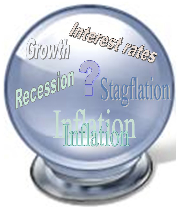
 Last year was far from the picture of economic stability that all governments would hope for. Instead, the overarching theme of 2022 was uncertainty, which overshadowed many economic predictions throughout the year. The Collins English Dictionary announced that their word of the year for 2022 is ‘permacrisis’, which is defined as ‘an extended period of instability and insecurity’.
For the UK, 2022 was an eventful year, seeing two changes in prime minister, economic stagnation, financial turmoil, rampant inflation and a cost of living crisis. However, the UK was not alone in its economic struggles. Many believe that it is a minor miracle that the world did not experience a systemic financial crisis in 2022.
Russia’s invasion of Ukraine has led to the biggest land war in Europe since 1945, the most serious risk of nuclear escalation since the Cuban missile crisis and the most far-reaching sanctions regime since the 1930s. Soaring food and energy costs have fuelled the highest rates of inflation since the 1980s and the biggest macroeconomic challenge in the modern era of central banking (with the possible exception of the financial crisis of 2007–8 and its aftermath). For decades we have lived with the assumptions that nuclear war was never going to happen, inflation will be kept low and rich countries will not experience an energy crisis. In 2022 all of these assumptions and more have been shaken.
With the combination of rising interest rates and a massive increase in geopolitical risk, the world economy did well to survive as robustly as it did. However, with public and private debt having risen to record levels during the now-bygone era of ultra-low interest rates and with recession risks high, the global financial system faces a huge stress test.
Government pledges
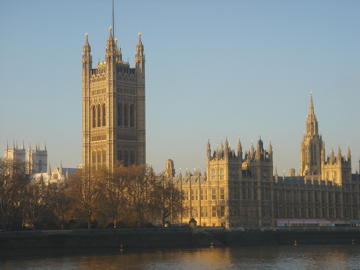 Rishi Sunak, the UK Prime Minister, started 2023 by setting out five pledges: to halve inflation, boost economic growth, cut national debt as a percentage of GDP, and to address NHS waiting lists and the issue of immigrants arriving in small boats. Whilst most would agree that meeting these pledges is desirable, a reduction in inflation is forecast to happen anyway, given the monetary policy being pursued by the Bank of England and an easing of commodity prices; and public-sector debt as a percentage of GDP is forecast to fall from 2024/25.
Success in meeting the first four pledges will partly depend on the effects of the current industrial action by workers across the UK. How soon will the various disputes be settled and on what terms? What will be the implications for service levels and for inflation?
A weak global economy
 Success will also depend on the state of the global economy, which is currently very fragile. In fact, it is predicted that a third of the global economy will be hit by recession this year. The head of the IMF has warned that the world faces a ‘tougher’ year in 2023 than in the previous 12 months. Such comments suggest the IMF is likely soon to cut its economic forecasts for 2023 again. The IMF already cut its 2023 outlook for global economic growth in October, citing the continuing drag from the war in Ukraine, as well as inflationary pressures and interest rate rises by major central banks.
The World Bank has also described the global economy as being ‘on a razor’s edge’ and warns that it risks falling into recession this year. The organisation expects the world economy to grow by just 1.7% this year, which is a sharp fall from an estimated 2.9% in 2022 according to the Global Economic Prospects report (see link below). It has warned that if financial conditions tighten, then the world’s economy could easily fall into a recession. If this becomes a reality, then the current decade would become the first since the 1930s to include two global recessions. Growth forecasts have been lowered for 95% of advanced economies and for more than 70% of emerging market and developing economies compared with six months ago. Given the global outlook, it is no surprise that the UK economy is expected to face a prolonged recession with declining growth and increased unemployment.
The current state of the UK economy
Despite all the concerns, official figures show that, even though households have been squeezed by rising prices, UK real GDP unexpectedly grew in November, by 0.1%. This has been explained by a boost to bars and restaurants from the World Cup as people went out to watch the football and also by demand for services in the tech sector.
At first sight, the UK’s cost of living crisis might look fairly mild compared to other countries. Its inflation rate was 10.7% in November 2022, compared to 12.6% in Italy, 16% in Poland and over 20% in Hungary and Estonia. But UK inflation is still way above the Bank of England’s 2% target. The Bank went on to tighten monetary policy further, by increasing interest rates to 3.5% in December. Further rate rises are expected in 2023. In fact, the markets and the Bank both expect the main rate to reach 5.2% by the end of this year. With the consequent squeeze on real incomes, the Bank of England expects a recession in the UK this year – possibly lasting until mid-2024.
 The UK is also affected by global interest rates, which affect global growth. Global interest rates average 5%. A 1 percentage point increase would reduce global growth this year from 1.7% to 0.6%, with per capita output contracting by 0.3%, once changes in population are taken into account. This would then meet the technical definition of a global recession. This means that the Bank’s November economic forecast, which was based on a Bank Rate of 3%, may worsen due to an even larger contraction than previously expected. The resulting drop in spending and investment by people and businesses could then cause inflation to come down faster than the Bank had predicted when rates were at 3%.
There could be some positive news however, that may help bring down inflation in addition to rate rises. There has been some appreciation in the pound since the huge drop caused by the September mini-budget that had brought its value to a nearly 40-year low. This will help to reduce inflation by reducing the price of imports.
As far as workers are concerned, pay increases have been broadly contained, with 2022 being one of the worst years in decades for UK real wage growth. Limiting pay rises can have a deflationary effect because people have less to spend, but it also weighs on economic growth and productivity. Despite the impact on inflation, there is a lot of unrest across the UK, with strike action continuing to be at the forefront of the news. Strikes over pay and conditions continue in various sectors in 2023, including transport, health, education and the postal service. Strikes and industrial action have a negative effect on the wider economy. If wages are stagnating and the economy is not performing well, productivity will suffer as workers are less motivated and less investment in new equipment takes place.
Financial stresses
 The UK economy is also under threat of a prolonged recession due to the proportion of households that lack insulation against financial setbacks. This proportion is unusually large for a wealthy economy. A survey conducted prior to the pandemic, found that 3 million people in the UK would fall into poverty if they missed one pay cheque, with the country’s high housing costs being a key source of vulnerability. Another survey recently suggested that one-third of UK adults would struggle if their costs rose by just £20 a month.
The pandemic itself meant that over 4 million households have taken on additional debt, with many now falling behind on repaying it. This, combined with recent jumps in energy and food bills, could push many over the edge, especially if heating costs remain high when the present government cap on energy prices ends in April.
However, there could be some better news for households with the easing of COVID restrictions in China. This could have a positive impact on the UK economy if it helps ease supply-chain disruptions occurring since the height of the global pandemic. It could reduce inflationary pressure in the UK and other countries that trade with China by making it easier – and therefore less costly – for people to get hold of goods.
Articles
Reports
Questions
- Define the term ‘deflation’.
- Explain how an appreciation of the pound is good for inflation.
- Discuss the wider economic impacts of industrial strike action.
- Why is it important for the government to keep wages contained?
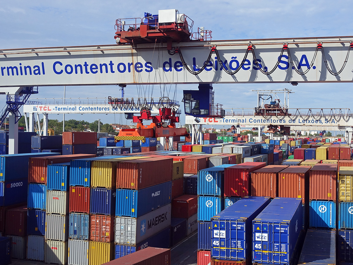 Over the decades, economies have become increasingly interdependent. This process of globalisation has involved a growth in international trade, the spread of technology, integrated financial markets and international migration.
When the global economy is growing, globalisation spreads the benefits around the world. However, when there are economic problems in one part of the world, this can spread like a contagion to other parts. This was clearly illustrated by the credit crunch of 2007–8. A crisis that started in the sub-prime market in the USA soon snowballed into a worldwide recession. More recently, the impact of Covid-19 on international supply chains has highlighted the dangers of relying on a highly globalised system of production and distribution. And more recently still, the war in Ukraine has shown the dangers of food and fuel dependency, with rapid rises in prices of basic essentials having a disproportionate effect on low-income countries and people on low incomes in richer countries.
Moves towards autarky
So is the answer for countries to become more self-sufficient – to adopt a policy of greater autarky? Several countries have moved in this direction. The USA under President Trump pursued a much more protectionist agenda than his predecessors. The UK, although seeking new post-Brexit trade relationships, has seen a reduction in trade as new barriers with the EU have reduced UK exports and imports as a percentage of GDP.  According to the Office for Budget Responsibility’s November 2022 Economic and Fiscal Outlook, Brexit will result in the UK’s trade intensity being 15 per cent lower in the long run than if it had remained in the EU.
Many European countries are seeking to achieve greater energy self-sufficiency, both as a means of reducing reliance on Russian oil and gas, but also in pursuit of a green agenda, where a greater proportion of energy is generated from renewables. More generally, countries and companies are considering how to reduce the risks of relying on complex international supply chains.
Limits to the gains from trade
The gains from international trade stem partly from the law of comparative advantage, which states that greater levels of production can be achieved by countries specialising in and exporting those goods that can be produced at a lower opportunity cost and importing those in which they have a comparative disadvantage. Trade can also lead to the transfer of technology and a downward pressure on costs and prices through greater competition.
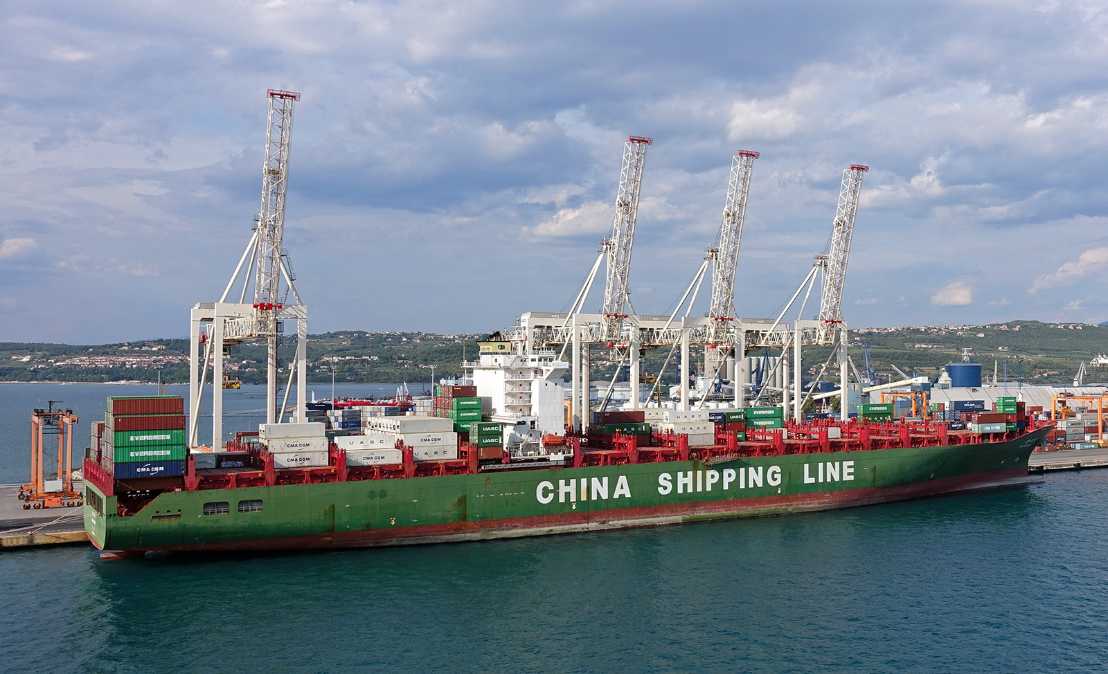 But trade can increase dependence on unreliable supply sources. For example, at present, some companies are seeking to reduce their reliance on Taiwanese parts, given worries about possible Chinese actions against Taiwan.
Also, governments have been increasingly willing to support domestic industries with various non-tariff barriers to imports, especially since the 2007–8 financial crisis. Such measures include subsidies, favouring domestic firms in awarding government contracts and using regulations to restrict imports. These protectionist measures are often justified in terms of achieving security of supply. The arguments apply particularly starkly in the case of food. In the light of large price increases in the wake of the Ukraine war, many countries are considering how to increase food self-sufficiency, despite it being more costly.
Also, trade in goods involves negative environmental externalities, as freight transport, whether by sea, air or land, involves emissions and can add to global warming. In 2021, shipping emitted over 830m tonnes of CO2, which represents some 3% of world total CO2 emissions. In 2019 (pre-pandemic), the figure was 800m tonnes. The closer geographically the trading partner, the lower these environmental costs are likely to be.
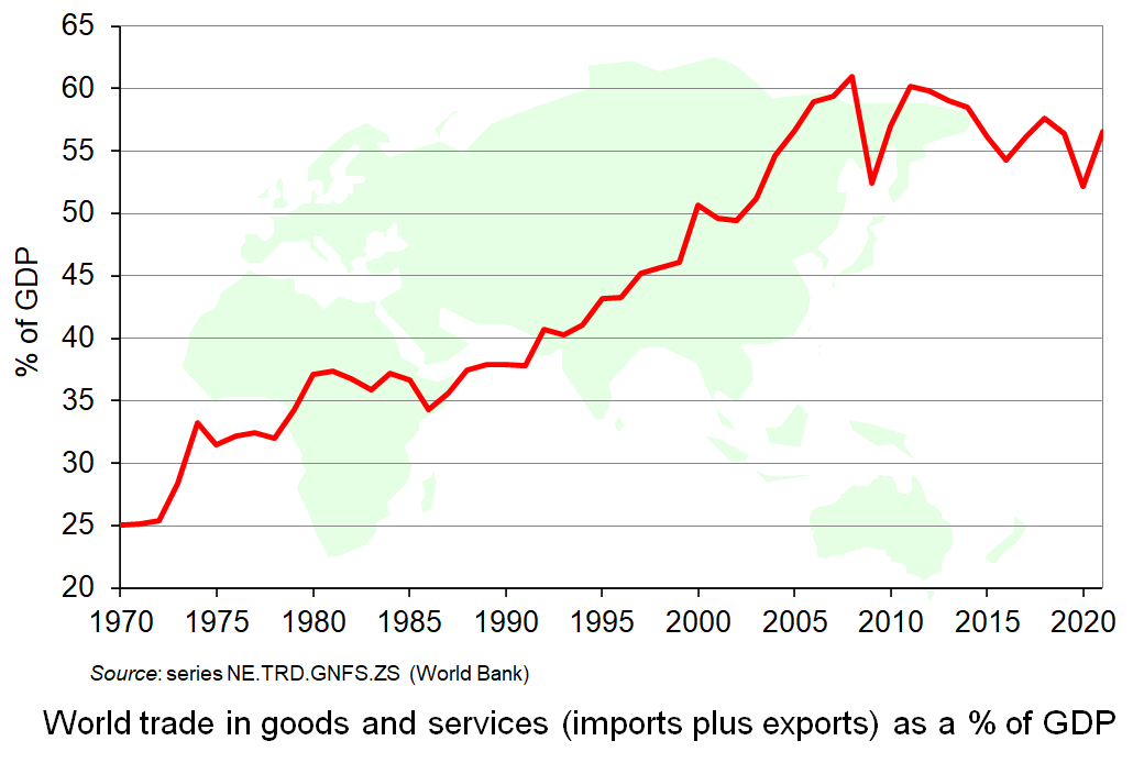 The problems with a globally interdependent world have led to world trade growing more slowly than world GDP in recent years after decades of trade growth considerably outstripping GDP growth. Trade (imports plus exports) as a percentage of GDP peaked at just over 60% in 2008. In 2019 and 2021 it was just over 56%. This is illustrated in the chart (click here for a PowerPoint). Although trade as a percentage of GDP rose slightly from 2020 to 2021 as economies recovered from the pandemic, it is expected to have fallen back again in 2022 and possibly further in 2023.
But despite this reduction in trade as a percentage of GDP, with de-globalisation likely to continue for some time, the world remains much more interdependent than in the more distant past (as the chart shows). Greater autarky may be seen as desirable by many countries as a response to the greater economic and political risks of the current world, but greater autarky is a long way from complete self-sufficiency. The world is likely to remain highly interdependent for the foreseeable future. Reports of the ‘death of globalisation’ are premature!
Podcasts
Articles
Report
Questions
- Explain the law of comparative advantage and demonstrate how trade between two countries can lead to both countries gaining.
- What are the main economic problems arising from globalisation?
- Is the answer to the problems of globalisation to move towards greater autarky?
- Would the expansion/further integration of trading blocs be a means of exploiting the benefits of globalisation while reducing the risks?
- Is the role of the US dollar likely to decline over time and, if so, why?
- Summarise Karl Polanyi’s arguments in The Great Transformation (see the Daniel W. Drezner article linked below). How well do they apply to the current world situation?
 On 23 September, the new Chancellor of the Exchequer, Kwasi Kwarteng, announced his mini-Budget. It revealed big tax-cutting plans with the aim of stimulating economic growth. See the blog From Reaganomics to Trussonomics for details. However, the announcement triggered a crisis of confidence in the markets. The government says the measures will kickstart economic growth, but with the tax cuts funded through extra government borrowing, markets have raised alarm over the plans, sending the pound plunging.
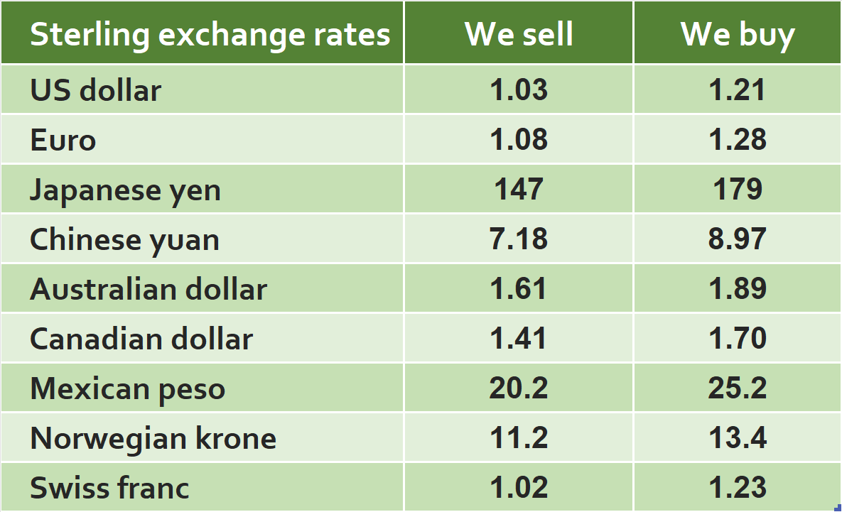
On Monday 26 September, traders in the UK awoke to see that the pound had fallen to the new lowest level on record against the dollar of $1.03. Although it came at a time when the markets expected the pound to weaken, the announcement pushed a fall in the pound beyond previous expectations. Concerns about where the extra money would come from to pay for the tax cuts were reflected in market movements. A weaker currency suggests investors’ faith in a country’s economic prospects is wavering.
What does a falling pound mean?
The pound’s value affects everyone – from shoppers to business owners and investors. The main impacts of the falling pound include:
- Higher prices. A fall in the value of the pound will increase the price of goods and services imported into the UK from overseas. When the pound is weak against the dollar, it costs more for companies in the UK to buy things such as food, raw materials or parts from abroad. Firms are likely then to pass on some or all those higher costs to their customers.
- Higher mortgage repayments. By increasing inflation, a falling pound is likely to push the Bank of England to raise interest rates to counter this. With two million people in the UK on a tracker or variable rate mortgage, monthly costs could increase substantially. Lenders are also likely to increase the rates charged on credit cards, bank loans or car loans.
- Further pressure on energy costs. The price of all of the gas that the UK uses is based on the dollar – even if the gas is produced in the UK. As oil prices are based on the dollar, petrol and diesel could also be more expensive for UK drivers as it costs more to be imported by fuel companies. Although the dollar price of oil has been falling in recent weeks, consumers are not likely to see the benefit at the pump due to the slide in the value of the pound.
- Stronger sales for UK firms who sell goods abroad. Some businesses in the UK could get a boost from a fall in the value of the pound. A cheaper pound makes it less expensive for people from around the globe to buy goods and services from British firms, making them more competitive.
- More expensive trips abroad. The plunge in the pound means that people’s holiday money won’t stretch as far, particularly for anyone planning a trip to the USA. The depreciation of the pound could also see airlines face sharply increased costs, with fuel and aircraft leases often denominated in dollars.
Threat to confidence
The Bank of England said a weaker outlook for the UK economy as well as a stronger dollar were putting pressure on sterling. However, market responses were clear that Kwarteng’s mini-Budget was threatening to undermine confidence in the UK. The pound plunged to its lowest since Britain went decimal in 1971, as belief in the UK’s economic management and assets evaporated.
By Tuesday 27 September, there were expectations that the Bank of England would have to raise interest rates to counter the extra spending in the mini-Budget. Economists from the City suggested the slump in the pound would not just force the Bank of England into raising rates at the next MPC announcement in November, but to intervene now by announcing an emergency interest rate rise to support the currency. This sent mortgage activity into a frenzy as brokers worked around the clock to help clients secure deals before lenders pulled their products or replaced them with more expensive ones. By the end of the week there were 40% fewer products available than before the mini-Budget.
The Bank of England
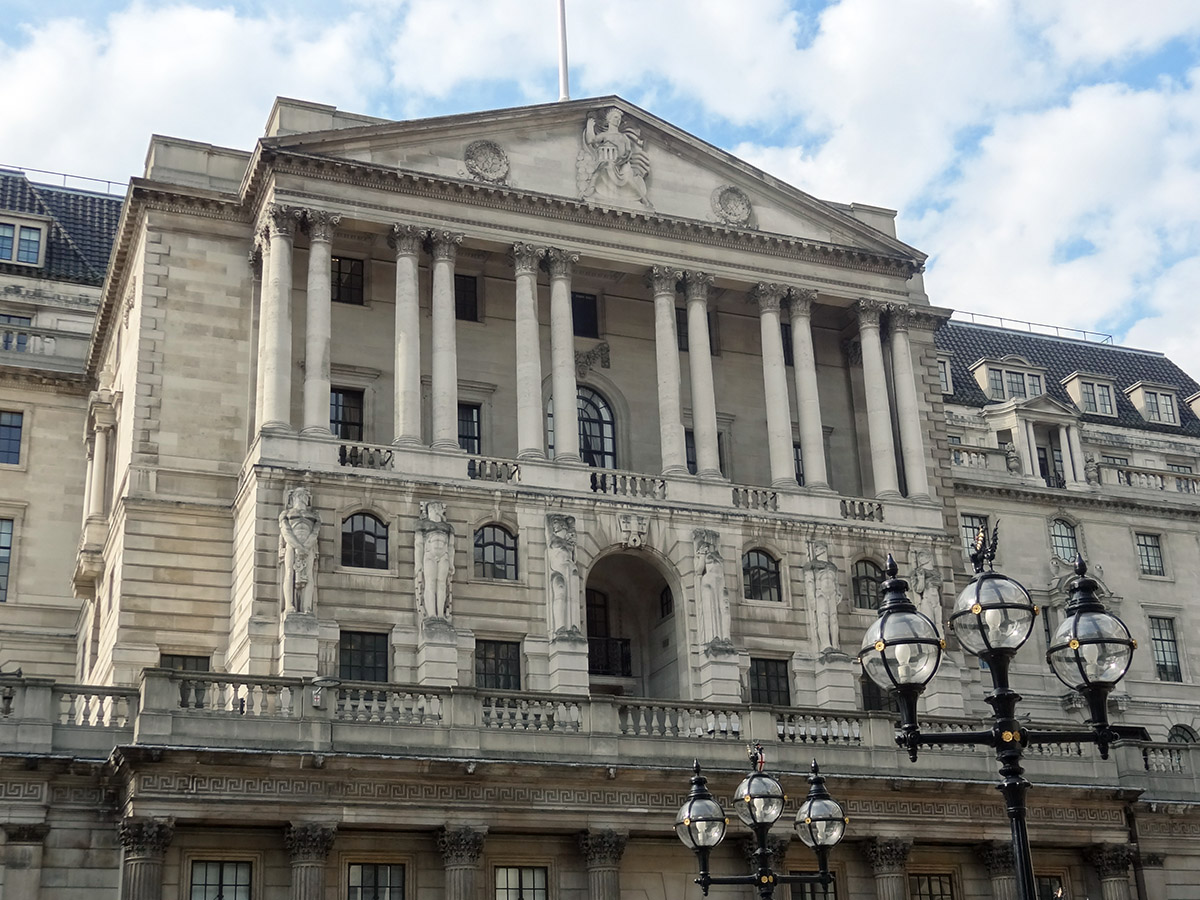 In August, the Bank predicted that the UK would go into recession, lasting some 15 months. It did so as it raised interest rates by the highest margin in 27 years (0.5 percentage points) in a bid to keep soaring prices under control. Higher interest rates can make borrowing more expensive, meaning people have less money to spend and prices will stop rising as quickly. The Bank of England is expected to raise interest rates by an even larger amount to combat the inflationary impact of the mini-Budget, as a weakening pound drives up costs of imports. The money markets are pricing a doubling of UK interest rates to more than 5% by next summer.
On Thursday 29 September the cost of government borrowing was rising to levels many economists thought were concerning. After the mini-Budget, the UK Debt Management Office, which borrows on behalf of the government by issuing new government bonds (‘gilts’), plans to raise an additional £72bn before next April, raising the financing remit in 2022/23 to £234bn. The investors in bonds are mainly large institutions, such as pension funds.
New bonds are issued at a fixed payment per annum based on the face value. If interest rates rise, then new bonds must pay a higher amount per annum to attract purchasers. Old bonds with a relatively low payment per year will fall in value. For example, if a £100 bond issued a while back paid £2 per annum (a nominal 2%) and interest rates on equivalent assets rose to 4%, the market price of the bond would fall to £50, as £2 per annum is 4% of £50. This percentage of the market price (as opposed to the face value) is known as the ‘yield’. With worries about the rise in government borrowing, bond prices fell and yields correspondingly rose. Investors were demanding much higher interest rates to lend to the UK government.
 The Investment Director at JM Finn compared investing in government bonds to sloths, they’re low risk and typically don’t move. This is because lending to the UK is usually considered as an ultra-safe bet. However, some bonds fell in price by 20% in two days (26–28 September).
There was concern that the mini-Budget threatened the financial health of Britain’s biggest pensions and insurance companies, which together manage trillions of pounds of people’s cash. These companies hold large amounts of UK government bonds and the fall in their price was significantly reducing the value of their assets.
The Bank of England thus announced that it would step in to calm markets, warning that continued volatility would be a ‘material risk to UK financial stability’. The Bank would start buying government bonds at an ‘urgent pace’ to help push their price back up and restore orderly market conditions. It would set aside £65bn to buy bonds over 13 working days. It is hoped that the Bank’s action will now ease the pressure on pension funds and insurance companies.
But the purchase of bonds increases money supply. This was the process by which money supply was increased during periods of quantitative easing (QE). Increasing money supply, while helping to dampen the rise in interest rates and stabilise the financial markets, is likely to lead to higher inflation. The Bank of England had previously planned to do the opposite: to engage in quantitative tightening (QT), which involves selling some of the stock of (old) bonds which the Bank had accumulated during the various rounds of QE.
Despite the Bank of England’s action which helped to curb the fall in the sterling exchange rate, some analysts warned it could fall further and could even reach parity with the dollar. There are concerns that the Bank is simply firefighting, rather than being able to solve the wider problems. There is now growing pressure on the government to make clear the financial cost of its tax cuts and spending plans.
Criticism from the IMF
 There has been widespread criticism of the government’s plan, with the International Monetary Fund warning on Tuesday 27 September that the measures were likely to fuel the cost-of-living crisis and increase inequality. The stinging rebuke from the IMF arrived at the worst moment for the UK government. The IMF works to stabilise the global economy and one of its key roles is to act as an early economic warning system. It said it understood the package aimed to boost growth, but it warned that the cuts could speed up the pace of price rises, which the UK’s central bank is trying to bring down. In an unusually outspoken statement, the IMF said the proposal was likely to increase inequality and add to pressures pushing up prices.
Mark Carney, the former Governor of the Bank of England also criticised the government, accusing them of ‘undercutting’ the UK’s key economic institutions. Mr Carney said that while the government was right to want to boost economic growth, ‘There is a lag between today and when that growth might come.’ He also criticised the government for undercutting various institutions that underpin the overall approach, including not having an OBR forecast.
What is next for the economy?
Before the announcement, the Bank had expected the economy to shrink in the last three months of 2022 and keep shrinking until the end of 2023. However, some economists believe the UK could already be in recession. The impacts of the mini-Budget have so far not alleviated fears of the UK diving into recession. However, the Governor of the Bank of England, Andrew Bailey, also warned that little could be done to stop the UK falling into a recession this year as the war in Ukraine continued. He added that it would ‘overwhelmingly be caused by the actions of Russia and the impact on energy prices’.
Despite the external pressures on the economy, it is clear that recent market activity has damaged confidence. The Bank has already said it will ‘not hesitate’ to hike interest rates to try to protect the pound and stem surging prices. Some economists have predicted the Bank of England will raise the interest rate from the current 2.25% to 5.75% by next spring.
The Bank’s action of emergency bond purchases helped provide Kwarteng with some respite from the financial markets after three days of turmoil, which included strong criticism of the mini-Budget from the International Monetary Fund, about 1000 mortgage products pulled and interest rates on UK government bonds hitting their highest level since 2008.
On 3 October, at the start of the Conservative Party annual conference, Kwarteng announced that the planned cut in the top rate of income tax from 45% to 40% would not go ahead. This showed that the government would change course if pressure was strong enough. That day, the sterling exchange rate against the dollar appreciated by around 0.5% to around $1.12.
But this was not enough. The pressure was still on the government. There were urgent calls from the House of Commons Treasury Select Committee to bring forward the government’s financial statement, which was not due until 23 November, by at least a month. The government was urged to publish growth forecasts as soon as possible to help calm the markets. In response, on 4 October the government agreed to bring the financial statement forward to late October along with the forecasts of its impacts from the OBR.
However, Truss and Kwarteng have so far resisted this pressure to bring analysis of their tax plans forward. They have refused independent analysis of their plans until more than six weeks after receiving them, despite more calls from Tory MPs for Downing Street to reassure the markets. The Prime Minister and Chancellor said they would only publish the independent forecasts on 23 November alongside a fiscal statement, despite them being ready on 7 October.
Longer term impacts
Amongst all the activity in the week following the mini-Budget, there are real concerns of the longer-term impacts the budget will have on the economy. Some experts predict that the lasting effects of the ‘mini’ Budget will be felt far beyond the trading floors. Large tax cuts the government claimed would boost growth have instead convinced markets the UK’s entire macroeconomic framework is under threat. Although this turmoil has been the short-term result, it’s important to step back and think about how the effects of this abrupt shift in economic policy will be felt far beyond the trading floors.
 Sterling’s partial recovery a few days after the mini-Budget reflects an increased confidence that there will be a large interest rate rise coming on November 3. However, the bleak economic outlook has removed any fiscal headroom the government may have had. The largest tax cuts in five decades need funding, while spooking the markets means another £12.5bn a year added to the debt interest bill. However, Kwarteng remains committed to debt falling eventually.
It is estimated that there needs to be a fiscal tightening of around £37–£47bn by 2026/27. Even more could be required to ensure that tax revenues cover day-to-day spending or for even a small margin for error. Many have therefore called for a U-turn on the measures announced in the mini-Budget beyond abolishing the cut to the top rate of income tax. Performing a U-turn on some of the tax cuts would make the fiscal tightening much more achievable. However, it could be politically detrimental. Much lower taxes will mean less public spending. Some suggest that this trade-off was ignored when those tax cuts were announced, but market pressure has now put it centre stage.
The Prime Minister has since admitted that mistakes were made in the controversial ‘mini’ Budget that sparked market turmoil in the last week of September. However, a day before reversing the cut in the top rate of income tax, she said she would not retreat on her plan to deliver £45bn of unfunded tax cuts, insisting it would help deliver growth, but admitted: ‘We should have laid the ground better and I have learned from that.’
Articles
- Pound hits all-time low against dollar after mini-budget rocks markets
The Guardian, Graeme Wearden (26/9/22)
- The pound: Why is it falling?
BBC News, Tom Edgington (27/9/22)
- Falling pound: What does it mean for me and my finances?
BBC News, Lora Jones (28/9/22)
- Bank of England steps in to calm markets
BBC News, Daniel Thomas and Noor Nanji (29/9/22)
- Government is undercutting UK institutions, says former Bank governor
BBC News, Dearbail Jordan (30/9/22)
- Bank of England in £65bn scramble to avert financial crisis
The Guardian, Larry Elliott, Pippa Crerar and Richard Partington (28/9/22)
 From mini-budget to market turmoil: Kwasi Kwarteng’s week – video timeline
The Guardian, Elena Morresi and Monika Cvorak plus sources as credited (30/9/22)
- Truss and Kwarteng resist pressure to bring analysis of their tax plans forward
The Guardian, Rowena Mason and Aubrey Allegretti (30/9/22)
- Mark Carney accuses Truss government of undermining Bank of England
The Guardian, Kalyeena Makortoff (29/9/22)
- Lasting effects of ‘mini’ Budget will be felt far beyond the trading floors
The Times, Torsten Bell (1/10/22)
- ‘Big impact’: UK economic chaos, pound plunge hit businesses
ABC News, Sylvia Hui and Kelvin Chan (30/9/22)
- Bank of England bonds rescue has two ugly implications: more inflation and an even weaker pound
The Conversation, Costas Milas (30/9/22)
- Sterling hits all-time low: two things can turn this around but neither is straightforward
The Conversation, Jean-Philippe Serbera (26/9/22)
Questions
- Explain how the announced tax cut will stimulate economic growth.
- What is the impact of the weakened pound on UK households and businesses?
- Draw a diagram illustrating the way in which the $/£ exchange rate is determined.
- How is UK inflation likely to be affected by a depreciation of sterling?
- Are there any advantages of having a lower pound?
 World politicians, business leaders, charities and pressure groups are meeting in Davos at the 2022 World Economic Forum. Normally this event takes place in January each year, but it was postponed to this May because of Covid-19 and is the first face-to-face meeting since January 2020.
The meeting takes place amid a series of crises facing the world economy. The IMF’s Managing Director, Kristalina Georgieva, described the current situation as a ‘confluence of calamities’. Problems include:
- Continuing hangovers from Covid have caused economic difficulties in many countries.
- The bounceback from Covid has led to demand outpacing supply. The world is suffering from a range of supply-chain problems and shortages of key materials and components, such as computer chips.
- The war in Ukraine has not only caused suffering in Ukraine itself, but has led to huge energy and food price increases as a result of sanctions and the difficulties in exporting wheat, sunflower oil and other foodstuffs.
- Supply shocks have led to rising global inflation. This will feed into higher inflationary expectations, which will compound the problem if they result in higher prices and wages in response to higher costs.
- Central banks have responded by raising interest rates. These dampen an already weakened global economy and could push the world into recession.
- Global inequality is rising rapidly, both within countries and between countries, as Covid disruptions and higher food and energy prices hit the poor disproportionately. Poor people and countries also have a higher proportion of debt and are thus hit especially hard by higher interest rates.
- Global warming is having increasing effects, with a growing incidence of floods, droughts and hurricanes. These lead to crop failures and the displacement of people.
- Countries are increasingly resorting to trade restrictions as they seek to protect their own economies. These slow economic growth.
World leaders at Davos will be debating what can be done. One approach is to use fiscal policy. Indeed, Kristalina Georgieva said that her ‘main message is to recognise that the world must spend the billions necessary to contain Covid in order to gain trillions in output as a result’. But unless the increased expenditure is aimed specifically at tackling supply shortages and bottlenecks, it could simply add to rising inflation. Increasing aggregate demand in the context of supply shortages is not the solution.
 In the long run, supply bottlenecks can be overcome with appropriate investment. This may require both greater globalisation and greater localisation, with investment in supply chains that use both local and international sources.
International sources can be widened with greater investment in manufacturing in some of the poorer developing countries. This would also help to tackle global inequality. Greater localisation for some inputs, especially heavier or more bulky ones, would help to reduce transport costs and the consumption of fuel.
With severe supply shocks, there are no simple solutions. With less supply, the world produces less and becomes poorer – at least temporarily until supply can increase again.
Articles
Discussion (video)
Report
Questions
- Draw an aggregate demand and supply diagram (AD/AS or DAD/DAS) to illustrate the effect of a supply shock on output and prices.
- Give some examples of supply-side policies that could help in the current situation.
- What are the arguments for and against countries using protectionist policies at the current time?
- What policies could countries adopt to alleviate rapid rises in the cost of living for people on low incomes? What problems do these policies pose?
- What are the arguments for and against imposing a windfall tax on energy companies and using the money to support poor people?
- If the world slips into recession, should central banks and governments use expansionary monetary and fiscal policies?
 The suffering inflicted on the Ukrainian people by the Russian invasion is immense. But, at a much lower level, the war will also inflict costs on people in countries around the world. There will be significant costs to households in the form of even higher energy and food price inflation and a possible economic slowdown. The reactions of governments and central banks could put a further squeeze on living standards. Stock markets could fall further and investment could decline as firms lose confidence.
Russia is the world’s second largest oil supplier and any disruption to supplies will drive up the price of oil significantly. Ahead of the invasion, oil prices were rising. At the beginning of February, Brent crude was around $90 per barrel. With the invasion, it rose above $100 per barrel.
 Russia is also a major producer of natural gas. The EU is particularly dependent on Russia, which supplies 40% of its natural gas. With Germany halting approval of the major new gas pipeline under the Baltic from Russia to Germany, Nord Stream 2, the price of gas has rocketed. On the day of the invasion, European gas prices rose by over 50%.
Nevertheless, with the USA deciding not to extend sanctions to Russia’s energy sector, the price of gas fell back by 32% the next day. It remains to be seen just how much the supplies of oil and gas from Russia will be disrupted over the coming weeks.
Both Russia and Ukraine are major suppliers of wheat and maize, between them responsible for 14% of global wheat production and 30% of global wheat exports. A significant rise in the price of wheat and other grains will exacerbate the current rise in food price inflation.
Russia is also a significant supplier of metals, such as copper, platinum, aluminium and nickel, which are used in a wide variety of products. A rise in their price has begun and will further add to inflationary pressures and supply-chain problems which have followed the pandemic.
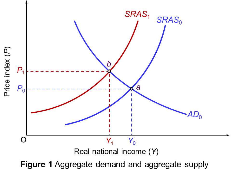 The effect of these supply shocks can be illustrated in a simple aggregate demand and supply diagram (see Figure 1), which shows a representative economy that imports energy, grain and other resources. Aggregate demand and short-run aggregate supply are initially given by AD0 and SRAS0. Equilibrium is at point a, with real national income (real GDP) of Y0 and a price index of P0.
The supply shock shifts short-run aggregate supply to SRAS1. Equilibrium moves to point b. The price index rises to P1 and real national income falls to Y1. If it is a ‘one-off’ cost increase, then the price index will settle at the new higher level and GDP at the new lower level provided that real aggregate demand remains the same. Inflation will be temporary. If, however, the SRAS curve continues to shift upwards to the left, then cost-push inflation will continue.
These supply-side shocks make the resulting inflation hard for policymakers to deal with. When the problem lies on the demand side, where the inflation is accompanied by an unsustainable boom, a contractionary fiscal and monetary policy can stabilise the economy and reduce inflation. But the inflationary problem today is not demand-pull inflation; it’s cost-push inflation. Disruptions to supply are both driving up prices and causing an economic slowdown – a situation of ‘stagflation’, or even an inflationary recession.
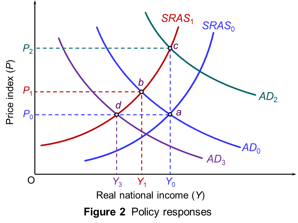 An expansionary policy, such as increasing bond purchases (quantitative easing) or increasing government spending, may help to avoid recession (at least temporarily), but will only exacerbate inflation. In Figure 2, aggregate demand shifts to AD2. Equilibrium moves to point c. Real GDP returns to Y0 (at least temporarily) but the price level rises further, to P2. (Click here for a PowerPoint of the diagram.)
A contractionary policy, such as raising interest rates or taxes, may help to reduce inflation but will make the slowdown worse and could lead to recession. In the diagram, aggregate demand shifts to AD3. Equilibrium moves to point d. The price level returns to P0 (at least temporarily) but real income falls further, to Y3.
In other words, you cannot tackle both the slowdown/recession and the inflation simultaneously by the use of demand-side policy. One requires an expansionary fiscal and/or monetary policy; the other requires fiscal and/or monetary tightening.
Then there are other likely economic stresses. If NATO countries respond by increasing defence expenditure, this will put further strain on public finances.
Sentiment is a key driver of the economy and prices. Expectations tend to be self-fulfilling. So if the war in Ukraine undermines confidence in stock markets and the real economy and further raises inflationary expectations, this pessimistic mood will tend in itself to drive down share prices, drive up inflation and drive down investment and economic growth.
Articles
- How will Russia’s invasion of Ukraine hit the global economy?
Financial Times, Chris Giles, Jonathan Wheatley and Valentina Romei (25/2/22)
- Ukraine conflict raises the possibility of stagflation
Financial Times, The Editorial Board (25/2/22)
- Five ways the Ukraine war could push up prices
BBC News, Laura Jones (5/3/22)
- Jason Furman cautions against reading too much into the initial market reactions to Russia’s invasion
interest.co.nz, Jason Furman (26/2/22)
- Putin’s war promises to crush the global economy with inflation and much slower growth
Market Watch, Nouriel Roubini (25/2/22)
- Roubini: 6 Financial, Economic Risks of Russia-Ukraine War
ThinkAdvisor, Janet Levaux (25/2/22)
- Fed tightening plans now contending with war, possible oil shock
Reuters, Howard Schneider and Jonnelle Marte (24/2/22)
- The invasion of Ukraine changed everything for Wall Street
CNN, Julia Horowitz (27/2/22)
- Why the Russian invasion will have huge economic consequences for American families
CNN, Matt Egan (24/2/22)
- European gas prices soar and oil tops $105 after Russia attacks Ukraine
Financial Times, Neil Hume, Emiko Terazono and Tom Wilson (24/2/22)
- Five essential commodities that will be hit by war in Ukraine
The Conversation, Sarah Schiffling and Nikolaos Valantasis Kanellos (24/2/22)
- Ukraine: ‘I’m surprised the oil price hasn’t hit US$130 a barrel yet’ – energy trading expert Q&A
The Conversation, Adi Imsirovic (25/2/22)
- Ukraine crisis: Warning UK energy bills could top £3,000 a year
BBC News, Michael Race (25/2/22)
- Putin’s energy shock: The economic realities of invasion
BBC News, Faisal Islam (25/2/22)
- Fears of UK food and fuel prices rising due to war
BBC News, Oliver Smith & Michael Race (26/2/22)
- Ukraine conflict: What is Swift and why is banning Russia so significant?
BBC News, Russell Hotten (27/2/22)
- Ukraine conflict: How reliant is Europe on Russia for oil and gas?
BBC News, Jake Horton & Daniele Palumbo (25/2/22)
- Ukraine crisis complicates ECB’s path to higher rates
Reuters, Francesco Canepa and Balazs Koranyi (24/2/22)
- Russia and the West are moving towards all out economic war
Al Jazeera, Maximilian Hess (24/2/22)
Questions
- If there is a negative supply shock, what will determine the size of the resulting increase in the price level and the rate of inflation over the next one or two years?
- How may expectations affect (a) the size of the increase in the price level; (b) future prices of gas and oil?
- Why did stock markets rise on the day after the invasion of Ukraine?
- Argue the case for and against relaxing monetary policy and delaying tax rises in the light of the economic consequences of the war in Ukraine.
 Last year was far from the picture of economic stability that all governments would hope for. Instead, the overarching theme of 2022 was uncertainty, which overshadowed many economic predictions throughout the year. The Collins English Dictionary announced that their word of the year for 2022 is ‘permacrisis’, which is defined as ‘an extended period of instability and insecurity’.
 Rishi Sunak, the UK Prime Minister, started 2023 by setting out five pledges: to halve inflation, boost economic growth, cut national debt as a percentage of GDP, and to address NHS waiting lists and the issue of immigrants arriving in small boats. Whilst most would agree that meeting these pledges is desirable, a reduction in inflation is forecast to happen anyway, given the monetary policy being pursued by the Bank of England and an easing of commodity prices; and public-sector debt as a percentage of GDP is forecast to fall from 2024/25.
  Success will also depend on the state of the global economy, which is currently very fragile. In fact, it is predicted that a third of the global economy will be hit by recession this year. The head of the IMF has warned that the world faces a ‘tougher’ year in 2023 than in the previous 12 months. Such comments suggest the IMF is likely soon to cut its economic forecasts for 2023 again. The IMF already cut its 2023 outlook for global economic growth in October, citing the continuing drag from the war in Ukraine, as well as inflationary pressures and interest rate rises by major central banks.
 The UK is also affected by global interest rates, which affect global growth. Global interest rates average 5%. A 1 percentage point increase would reduce global growth this year from 1.7% to 0.6%, with per capita output contracting by 0.3%, once changes in population are taken into account. This would then meet the technical definition of a global recession. This means that the Bank’s November economic forecast, which was based on a Bank Rate of 3%, may worsen due to an even larger contraction than previously expected. The resulting drop in spending and investment by people and businesses could then cause inflation to come down faster than the Bank had predicted when rates were at 3%.
 The UK economy is also under threat of a prolonged recession due to the proportion of households that lack insulation against financial setbacks. This proportion is unusually large for a wealthy economy. A survey conducted prior to the pandemic, found that 3 million people in the UK would fall into poverty if they missed one pay cheque, with the country’s high housing costs being a key source of vulnerability. Another survey recently suggested that one-third of UK adults would struggle if their costs rose by just £20 a month.
  Over the decades, economies have become increasingly interdependent. This process of globalisation has involved a growth in international trade, the spread of technology, integrated financial markets and international migration.
 According to the Office for Budget Responsibility’s November 2022 Economic and Fiscal Outlook, Brexit will result in the UK’s trade intensity being 15 per cent lower in the long run than if it had remained in the EU.
  But trade can increase dependence on unreliable supply sources. For example, at present, some companies are seeking to reduce their reliance on Taiwanese parts, given worries about possible Chinese actions against Taiwan.
  The problems with a globally interdependent world have led to world trade growing more slowly than world GDP in recent years after decades of trade growth considerably outstripping GDP growth. Trade (imports plus exports) as a percentage of GDP peaked at just over 60% in 2008. In 2019 and 2021 it was just over 56%. This is illustrated in the chart (click
 On 23 September, the new Chancellor of the Exchequer, Kwasi Kwarteng, announced his mini-Budget. It revealed big tax-cutting plans with the aim of stimulating economic growth. See the blog
  In August, the Bank predicted that the UK would go into recession, lasting some 15 months. It did so as it raised interest rates by the highest margin in 27 years (0.5 percentage points) in a bid to keep soaring prices under control. Higher interest rates can make borrowing more expensive, meaning people have less money to spend and prices will stop rising as quickly. The Bank of England is expected to raise interest rates by an even larger amount to combat the inflationary impact of the mini-Budget, as a weakening pound drives up costs of imports. The money markets are pricing a doubling of UK interest rates to more than 5% by next summer.
 The Investment Director at JM Finn compared investing in government bonds to sloths, they’re low risk and typically don’t move. This is because lending to the UK is usually considered as an ultra-safe bet. However, some bonds fell in price by 20% in two days (26–28 September).
  There has been widespread criticism of the government’s plan, with the International Monetary Fund warning on Tuesday 27 September that the measures were likely to fuel the cost-of-living crisis and increase inequality. The stinging rebuke from the IMF arrived at the worst moment for the UK government. The IMF works to stabilise the global economy and one of its key roles is to act as an early economic warning system. It said it understood the package aimed to boost growth, but it warned that the cuts could speed up the pace of price rises, which the UK’s central bank is trying to bring down. In an unusually outspoken statement, the IMF said the proposal was likely to increase inequality and add to pressures pushing up prices.
 Sterling’s partial recovery a few days after the mini-Budget reflects an increased confidence that there will be a large interest rate rise coming on November 3. However, the bleak economic outlook has removed any fiscal headroom the government may have had. The largest tax cuts in five decades need funding, while spooking the markets means another £12.5bn a year added to the debt interest bill. However, Kwarteng remains committed to debt falling eventually.
  World politicians, business leaders, charities and pressure groups are meeting in Davos at the
  In the long run, supply bottlenecks can be overcome with appropriate investment. This may require both greater globalisation and greater localisation, with investment in supply chains that use both local and international sources.
  The suffering inflicted on the Ukrainian people by the Russian invasion is immense. But, at a much lower level, the war will also inflict costs on people in countries around the world. There will be significant costs to households in the form of even higher energy and food price inflation and a possible economic slowdown. The reactions of governments and central banks could put a further squeeze on living standards. Stock markets could fall further and investment could decline as firms lose confidence.
 Russia is also a major producer of natural gas. The EU is particularly dependent on Russia, which supplies 40% of its natural gas. With Germany halting approval of the major new gas pipeline under the Baltic from Russia to Germany, Nord Stream 2, the price of gas has rocketed. On the day of the invasion, European gas prices rose by over 50%.
  The effect of these supply shocks can be illustrated in a simple aggregate demand and supply diagram (see Figure 1), which shows a representative economy that imports energy, grain and other resources. Aggregate demand and short-run aggregate supply are initially given by AD0 and SRAS0. Equilibrium is at point a, with real national income (real GDP) of Y0 and a price index of P0.
 An expansionary policy, such as increasing bond purchases (quantitative easing) or increasing government spending, may help to avoid recession (at least temporarily), but will only exacerbate inflation. In Figure 2, aggregate demand shifts to AD2. Equilibrium moves to point c. Real GDP returns to Y0 (at least temporarily) but the price level rises further, to P2. (Click