 Many developing countries are facing a renewed debt crisis. This is directly related to Covid-19, which is now sweeping across many poor countries in a new wave.
Between 2016 and 2020, debt service as a percentage of GDP rose from an average of 7.1% to 27.1% for South Asian countries, from 8.1% to 14.1% for Sub-Saharan African countries, from 13.1% to 42.3% for North African and Middle Eastern countries, and from 5.6% to 14.7% for East Asian and Pacific countries. These percentages are expected to climb again in 2021 by around 10% of GDP.
Incomes have fallen in developing countries with illness, lockdowns and business failures. This has been compounded by a fall in their exports as the world economy has contracted and by a 19% fall in aid in 2020. The fall in incomes has led to a decline in tax revenues and demands for increased government expenditure on healthcare and social support. Public-sector deficits have thus risen steeply.
And the problem is likely to get worse before it gets better. Vaccination roll-outs in most developing countries are slow, with only a tiny fraction of the population having received just one jab. With the economic damage already caused, growth is likely to be subdued for some time.
This has put developing countries in a ‘trilemma’, as the IMF calls it. Governments must balance the objectives of:
- meeting increased spending needs from the emergency and its aftermath;
- limiting the substantial increase in public debt;
- trying to contain rises in taxes.
Developing countries are faced with a difficult trade-off between these objectives, as addressing one objective is likely to come at the expense of the other two. For example, higher spending would require higher deficits and debt or higher taxes.
The poorest countries have little scope for increased domestic borrowing and have been forced to borrow on international markets. But such debt is costly. Although international interest rates are generally low, many developing countries have had to take on increasing levels of borrowing from private lenders at much higher rates of interest, substantially adding to the servicing costs of their debt.
Debt relief
 International agencies and groups, such as the IMF, the World Bank, the United Nations and the G20, have all advocated increased help to tackle this debt crisis. The IMF has allocated $100bn in lending through the Rapid Financing Instrument (RFI) and the Rapid Credit Facility (RCF) and nearly $500m in debt service relief grants through the Catastrophe Containment and Relief Trust (CCRT). The World Bank is increasing operations to $160bn.
The IMF is also considering an increase in special drawing rights (SDRs) from the current level of 204.2bn ($293.3bn) to 452.6bn ($650bn) – a rise of 121.6%. This would be the first such expansion since 2009. It has received the support of both the G7 and the G20. SDRs are reserves created by the IMF whose value is a weighted average of five currencies – the US dollar (41.73%), the euro (30.93%), the Chinese yuan (10.92%), the Japanese yen (8.33%) and the pound sterling (8.09%).
Normally an increase in SDRs would be allocated to countries according their IMF quotas, which largely depend on the size of their GDP and their openness. Any new allocation under this formula would therefore go mainly to developed countries, with developing economies getting only around $60bn of the extra $357bn. It has thus been proposed that developed countries give much of their allocation to developing countries. These could then be used to cancel debts. This proposal has been backed by Janet Yellen, the US Secretary of the Treasury, who said she would “strongly encourage G20 members to channel excess SDRs in support of recovery efforts in low-income countries, alongside continued bilateral financing”.
 The G20 countries, with the support of the IMF and World Bank, have committed to suspend debt service payments by eligible countries which request to participate in its Debt Service Suspension Initiative (DSSI). There are 73 eligible countries. The scheme, now extended to 31 December 2021, provides a suspension of debt-service payments owed to official bilateral creditors. In return, borrowers commit to use freed-up resources to increase social, health or economic spending in response to the crisis. As of April 2021, 45 countries had requested to participate, with savings totalling more than $10bn. The G20 has also called on private creditors to join the DSSI, but so far without success.
Despite these initiatives, the scale of debt relief (as opposed to extra or deferred lending) remains small in comparison to earlier initiatives. Under the Heavily Indebted Poor Countries initiative (HIPC, launched 1996) and the Multilateral Debt Relief Initiative (MDRI, launched 2005) more than $100bn of debt was cancelled.
Since the start of the pandemic, major developed countries have spent between $10 000 and $20 000 per head in stimulus and social support programmes. Sub-Saharan African countries on average are seeking only $365 per head in support.
Articles and blogs
Podcast
Report
Data
Questions
- Imagine you are an economic advisor to a developing country attempting to rebuild the economy after the coronavirus pandemic. How would you advise it to proceed, given the ‘trilemma’ described above?
- How does the News24 article define ‘smart debt relief’. Do you agree with the definition and the means of achieving smart debt relief?
- To what extent is it in the interests of the developed world to provide additional debt relief to poor countries whose economies have been badly affected by the coronavirus pandemic?
- Research ‘debt-for-nature swaps’. To what extent can debt relief for countries affected by the coronavirus pandemic be linked to tackling climate change?
 The LSE’s Centre for Economic Performance has just published a paper looking at the joint impact of Covid-19 and Brexit on the UK economy. Apart from the short-term shocks, both will have a long-term dampening effect on the UK economy. But they will largely affect different sectors.
Covid-19 has affected, and will continue to affect, direct consumer-facing industries, such as shops, the hospitality and leisure industries, public transport and personal services. Brexit will tend to hit those industries most directly involved in trade with Europe, the UK’s biggest trading partner. These industries include manufacturing, financial services, posts and telecommunications, mining and quarrying, and agriculture and fishing.
Despite the fact that largely different sectors will be hit by these two events, the total effect may be greater than from each individually. One of the main reasons for this is the dampening impact of Covid-19 on globalisation.  Travel restrictions are likely to remain tighter to more distant countries. And countries are likely to focus on trading within continents or regions rather than the whole world. For the UK, this, other things being equal, would mean an expansion of trade with the EU relative to the rest of the world. But, unless there is a comprehensive free-trade deal with the EU, the UK would not be set to take full advantage of this trend.
Another problem is that the effects of the Covid-19 pandemic have weakened the economy’s ability to cope with further shocks, such as those from Brexit. Depending on the nature (or absence) of a trade deal, Brexit will impose higher burdens on trading companies, including meeting divergent standards and higher administrative costs from greater form filling, inspections and customs delays.
Papers
Articles
Questions
- Referring to the LSE paper, give some examples of industries that are likely to be particularly hard hit by Brexit when the transition period ends? Explain why.
- Why have university finances been particularly badly affected by both Covid-19 and Brexit? Are there any other sectors that have suffered (or will suffer) badly from both events?
- Is there a scenario where globalisation in trade could start to grow again?
- Has Covid-19 affected countries’ comparative advantage in particular products traded with particular countries and, if so, how?
- The authors of the LSE report argue that ‘government policies to stimulate demand, support workers to remain in employment or find new employment, and to support businesses remain essential’. How realistic is it to expect the government to provide additional support to businesses and workers to deal with the shock of Brexit?
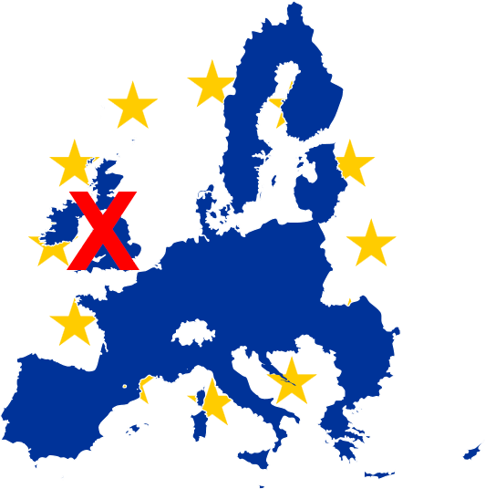 There have been many analyses of the economic effects of Brexit, both before the referendum and at various times since, including analyses of the effects of the deal negotiated by Theresa May’s government and the EU. But with the prospect of a no-deal Brexit on 31 October under the new Boris Johnson government, attention has turned to the effects of leaving the EU without a deal.
There have been two major analyses recently of the likely effects of a no-deal Brexit – one by the International Monetary Fund (IMF) and one by the Office for Budget Responsibility (OBR).
IMF analysis
The first was in April by the IMF as part of its 6-monthly World Economic Outlook. In Scenario Box 1.1. ‘A No-Deal Brexit’ on page 28 of Chapter 1, the IMF looked at two possible scenarios.
Scenario A assumes no border disruptions and a relatively small increase in UK sovereign and corporate spreads. Scenario B incorporates significant border disruptions that increase import costs for UK firms and households (and to a lesser extent for the European Union) and a more severe tightening in financial conditions.
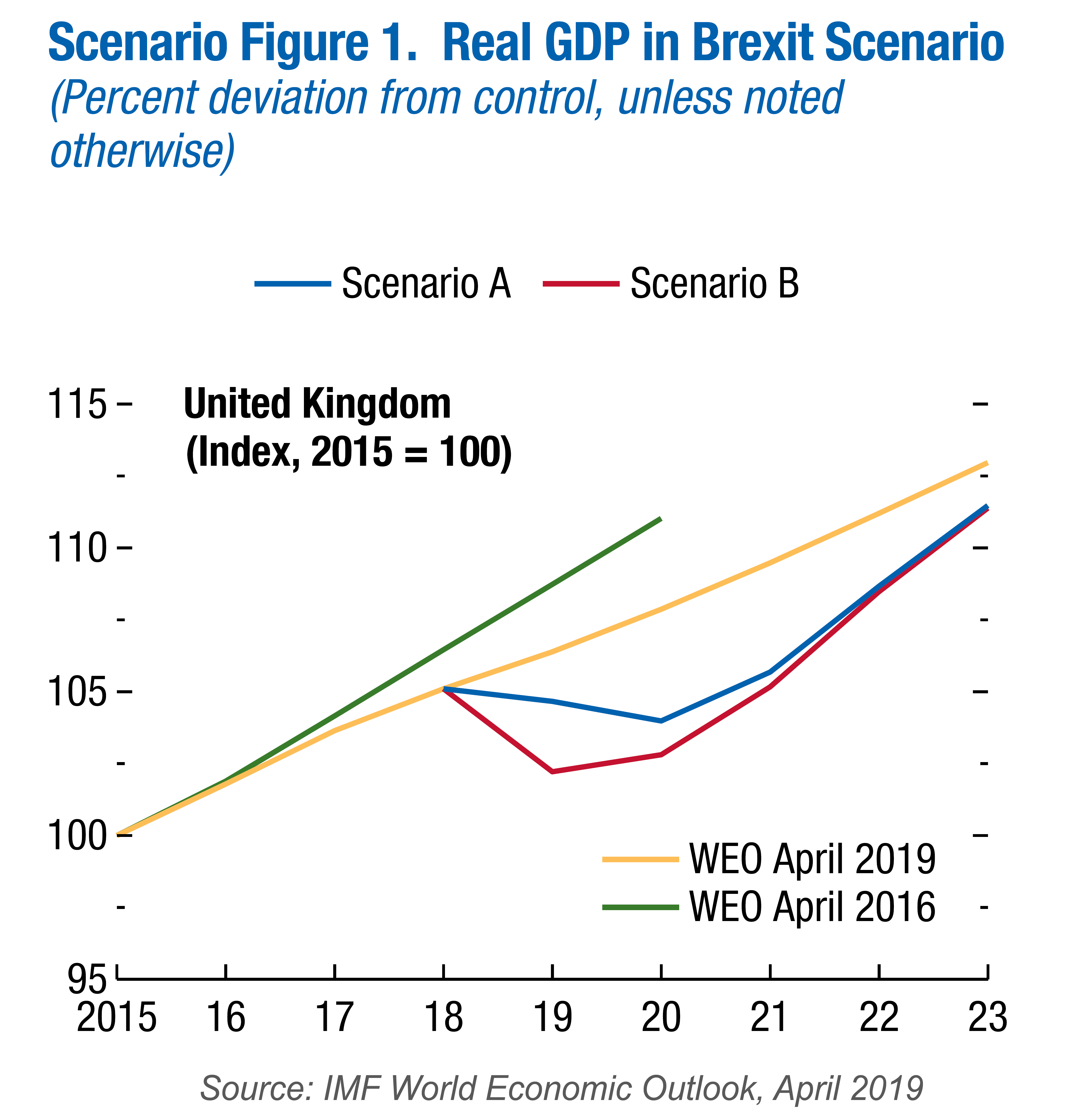 Under both scenarios, UK exports to the EU and UK imports from the EU revert to WTO rules. As a result, tariffs are imposed by mid-2020 or earlier. Non-tariff barriers rise at first but are gradually reduced over time. Most free-trade arrangements between the EU and other countries are initially unavailable to the UK (see the blog EU strikes major trade deals) but both scenarios assume that ‘new trade agreements are secured after two years, and on terms similar to those currently in place.’
Both scenarios also assume a reduction in net immigration from the EU of 25 000 per year until 2030. Both assume a rise in corporate and government bond rates, reflecting greater uncertainty, with the effect being greater in Scenario B. Both assume a relaxing of monetary and fiscal policy in response to downward pressures on the economy.
The IMF analysis shows a negative impact on UK GDP, with the economy falling into recession in late 2019 and in 2020. This is the result of higher trade costs and reduced business investment caused by a poorer economic outlook and increased uncertainty. By 2021, even under Scenario A, GDP is approximately 3.5% lower than it would have been if the UK had left the EU with the negotiated deal. For the rest of the EU, GDP is around 0.5% lower, although the effect varies considerably from country to country.
The IMF analysis makes optimistic assumptions, such as the UK being able to negotiate new trade deals with non-EU countries to replace those lost by leaving. More pessimistic assumptions would lead to greater costs.
OBR analysis
Building on the analysis of the IMF, the Office for Budget Responsibility considered the effect of a no-deal Brexit on the public finances in its biennial Fiscal risks report, published on 17 July 2019. This argues that, under the relatively benign Scenario A assumptions of the IMF, the lower GDP would result in annual public-sector net borrowing (PSNB) rising. By 2021/22, if the UK had left with the deal negotiated with the EU, PSNB would have been around £18bn. A no-deal Brexit would push this up to around £51bn.
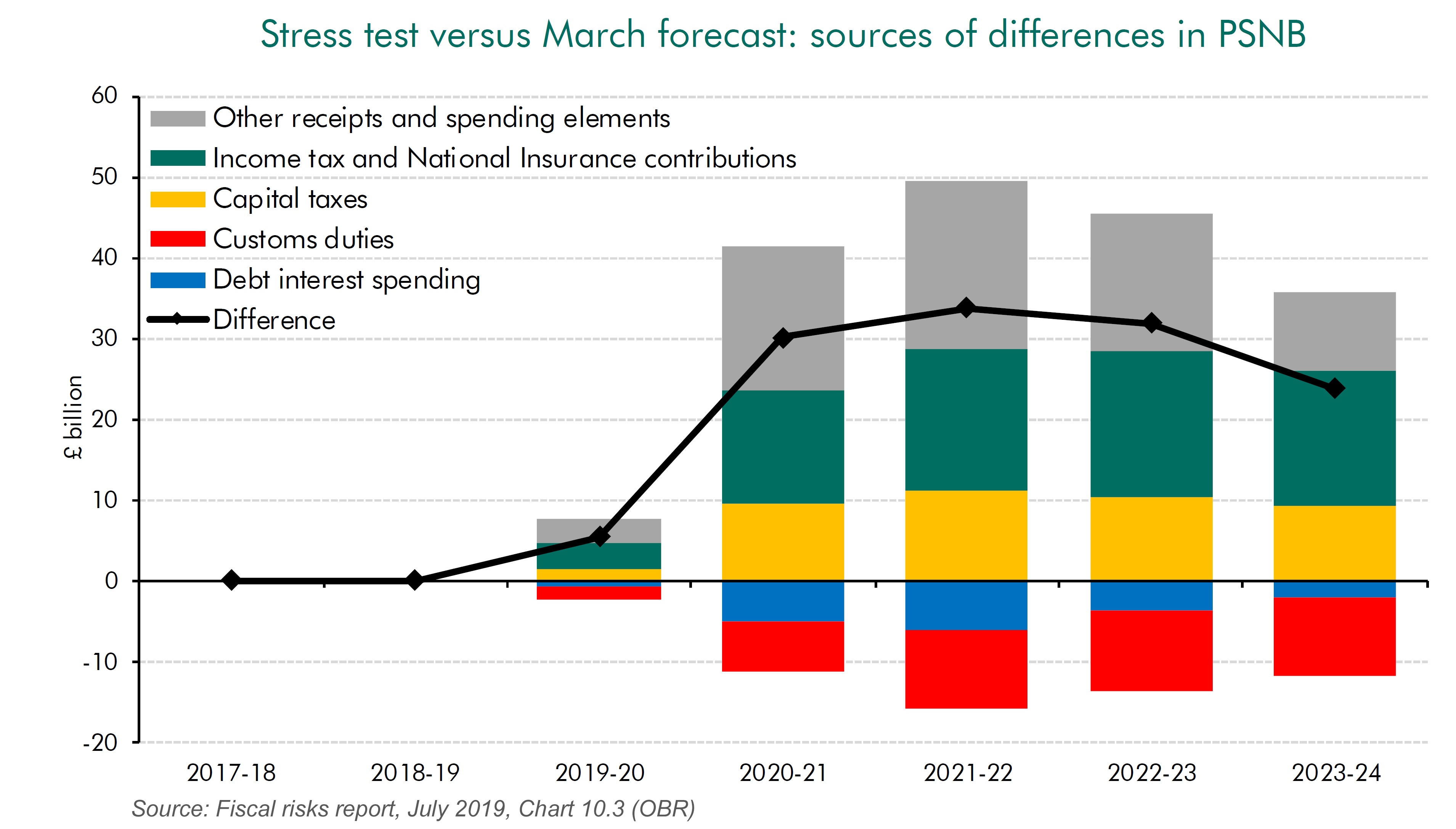
According to the OBR, the contributors to this rise in public-sector net borrowing of around £33bn are:
- A fall in income tax and national insurance receipts of around £16.5bn per year because of lower incomes.
- A fall in corporation tax and expenditure taxes, such as VAT, excise duties and stamp duty of around £22.5bn per year because of lower expenditure.
- A fall in capital taxes, such as inheritance tax and capital gains tax of around £10bn per year because of a fall in asset prices.
- These are offset to a small degree by a rise in customs duties (around £10bn) because of the imposition of tariffs and by lower debt repayments (of around £6bn) because of the Bank of England having to reduce interest rates.
The rise in PSNB would constrain the government’s ability to use fiscal policy to boost the economy and to engage in the large-scale capital projects advocated by Boris Johnson while making the substantial tax cuts he is proposing. A less optimistic set of assumptions would, of course, lead to a bigger rise in PSNB, which would further constrain fiscal policy.
Articles
Video
Reports
Questions
- What are the assumptions of the IMF World Economic Outlook forecasts for the effects of a no-deal Brexit? Do you agree with these assumptions? Explain.
- What are the assumptions of the analysis of a no-deal Brexit on the public finances in the OBR’s Fiscal risks report? Do you agree with these assumptions? Explain.
- What is the difference between forecasts and analyses of outcomes?
- For what reasons might growth over the next few years be higher than in the IMF forecasts under either scenario?
- For what reasons might growth over the next few years be lower than in the IMF forecasts under either scenario?
- For what reasons might public-sector net borrowing (PSNB) over the next few years be lower than in the OBR forecast?
- For what reasons might PSNB over the next few years be higher than in the OBR forecast?
 Consumer credit is borrowing by individuals to finance current expenditure on goods and services. Consumer credit is distinct from lending secured on dwellings (referred to more simply as ‘secured lending’). Consumer credit comprises lending on credit cards, lending through overdraft facilities and other loans and advances, for example those financing the purchase of cars. We consider here recent trends in the flows of consumer credit in the UK and discuss their implications.
Analysing consumer credit data is important because the growth of consumer credit has implications for the financial wellbeing or financial health of individuals and, of course, for financial institutions. As we shall see shortly, the data on consumer credit is consistent with the existence of credit cycles. Cycles in consumer credit have the potential to be not only financially harmful but economically destabilising. After all, consumer credit is lending to finance spending and therefore the amount of lending can have significant effects on aggregate demand and economic activity.
Data on consumer credit are available monthly and so provide an early indication of movements in economic activity. Furthermore, because lending flows are likely to be sensitive to changes in the confidence of both borrowers and lenders, changes in the growth of consumer credit can indicate turning points in the economy and, hence, in the macroeconomic environment.
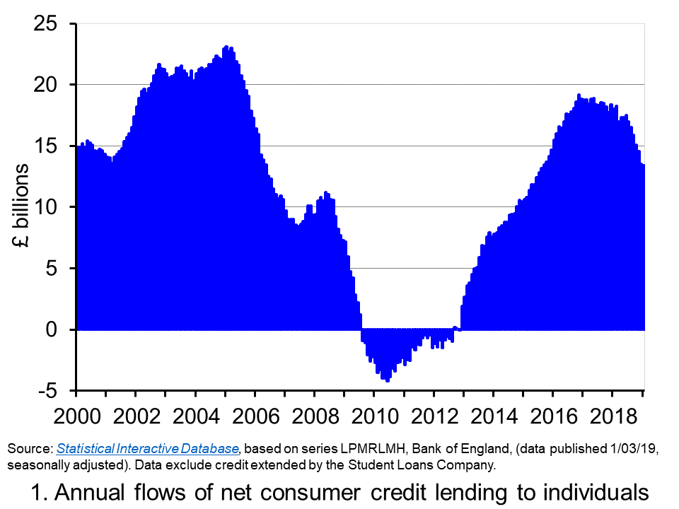 Chart 1 shows the annual flows of net consumer credit since 2000 – the figures are in £ billions. Net flows are gross flows less repayments. (Click here to download a PowerPoint copy of the chart.) In January 2005 the annual flow of net consumer credit peaked at £23 billion, the equivalent of just over 2.5 per cent of annual disposable income. This helped to fuel spending and by the final quarter of the year, the economy’s annual growth rate had reached 4.8 per cent, significantly about its long-run average of 2.5 per cent.
By 2009 net consumer credit flows had become negative. This meant that repayments were greater than additional flows of credit. It was not until 2012 that the annual flow of net consumer credit was again positive. Yet by November 2016, the annual flow of net consumer credit had rebounded to over £19 billion, the equivalent of just shy of 1.5 per cent of annual disposable income. This was the largest annual flow of consumer credit since September 2005.
Although the strength of consumer credit in 2016 was providing the economy with a timely boost to growth in the immediate aftermath of the referendum on the UK’s membership of the EU, it nonetheless raised concerns about its sustainability. Specifically, given the short amount of time that had elapsed since the financial crisis and the extreme levels of financial distress that had been experienced by many sectors of the economy, how susceptible would people and organisations be to a future economic slowdown and/or rise in interest rates?
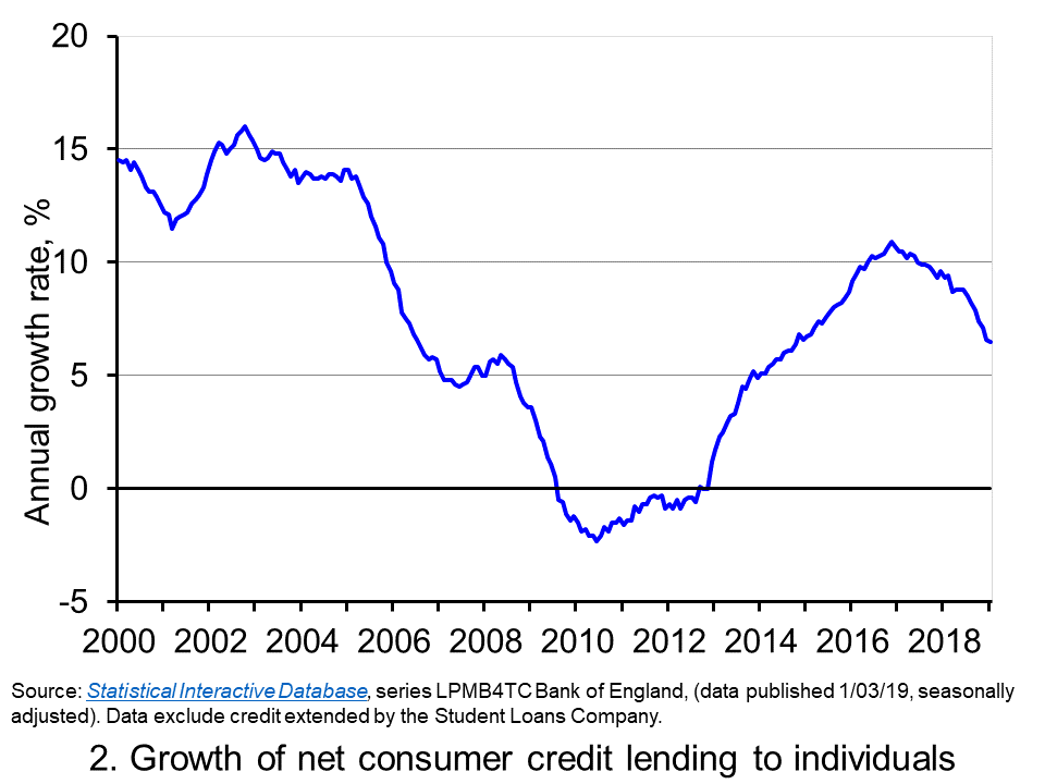 The extent to which the economy experiences consumer credit cycles can be seen even more readily by looking at the 12-month growth rate in the net consumer credit. In essence, this mirrors the growth rate in the stock of consumer credit. Chart 2 evidences the double-digit growth rates in net consumer credit lending experienced during the first half of the 2000s. Growth rates then eased but, as the financial crisis unfolded, they plunged sharply. (Click here to download a PowerPoint copy of the chart.)
Yet, as Chart 2 shows, consumer credit growth began to recover quickly from 2013 so that by 2016 the annual growth rate of net consumer credit was again in double figures. In November 2016 the 12-month growth rate of net consumer credit peaked at 10.9 per cent. Thereafter, the growth rate has continually eased. In January 2019 the annual growth rate of net consumer credit had fallen back to 6.5 per cent, the lowest rate since October 2014.
The easing of consumer credit is likely to have been influenced, in part, by the resumption in the growth of real earnings from 2018 (see Getting real with pay). Yet, it is hard to look past the economic uncertainties around Brexit.
Uncertainty tends to cause people to be more cautious. With the heightened uncertainty that has has characterised recent times, it is likely that for many people and businesses prudence has dominated impatience. Therefore, in summary, it appears that prudence is helping to steer borrowing along a downswing in the credit cycle. As it does, it helps to put a further brake on spending and economic growth.
Articles
Questions
- What is the difference between gross and net lending?
- Consider the argument that we should be worried more by excessive growth in consumer credit than on lending secured on dwellings?
- How could we measure whether different sectors of the economy had become financially distressed?
- What might explain why an economy experiences credit cycles?
- Explain how the growth in net consumer credit can affect economic activity?
- If people are consumption smoothers, how can credit cycles arise?
- What are the potential policy implications of credit cycles?
- It is said that when making financial decisions people face an inter-temporal choice. Explain what you understand this by this concept.
- If economic uncertainty is perceived to have increased how could this affect the consumption, saving and borrowing decisions of people?
 Today’s title is inspired from the British Special Air Service (SAS) famous catchphrase, ‘Who Dares Wins’ – similar variations of which have been adopted by several elite army units around the world. The motto is often credited to the founder of the SAS, Sir David Stirling (although similar phrases can be traced back to ancient Rome – including ‘qui audet adipiscitur’, which is Latin for ‘who dares wins’). The motto was used to inspire and remind soldiers that to successfully accomplish difficult missions, one has to take risks (Geraghty, 1980).
In the world of economics and finance, the concept of risk is endemic to investments and to making decisions in an uncertain world. The ‘no free lunch’ principle in finance, for instance, asserts that it is not possible to achieve exceptional returns over the long term without accepting substantial risk (Schachermayer, 2008).
 Undoubtedly, one of the riskiest investment instruments you can currently get your hands on is cryptocurrencies. The most well-known of them is Bitcoin (BTC), and its price has varied spectacularly over the past ten years – more than any other asset I have laid my eyes on in my lifetime.
The first published exchange rate of BTC against the US dollar dates back to 5 October 2009 and it shows $1 to be exchangeable for 1309.03 BTC. On 15 December 2017, 1 BTC was traded for $17,900. But then, a year later the exchange rate was down to just over $1 = $3,500. Now, if this is not volatility I don’t know what is!
In such a market, wouldn’t it be wonderful if you could somehow predict changes in market sentiment and volatility trends? In a hot-off-the press article, Shen et al (2019) assert that it may be possible to predict changes in trading volumes and realised volatility of BTC by using the number of BTC-related tweets as a measure of attention. The authors source Twitter data on Bitcoin from BitInfoCharts.com and tick data from Bitstamp, one of the most popular and liquid BTC exchanges, over the period 4/9/2014 to 31/8/2018.
According to the authors:
This measure of investor attention should be more informed than that of Google Trends and therefore may reflect the attention Bitcoin is receiving from more informed investors. We find that the volume of tweets are significant drivers of realised [price] volatility (RV) and trading volume, which is supported by linear and nonlinear Granger causality tests.
They find that, according to Granger causality tests, for the period from 4/9/2014 to 8/10/2017, past days’ tweeting activity influences (or at least forecasts) trading volume. While from 9/10/2017 to 31/8/2018, previous tweets are significant drivers/forecasters of not only trading volume but also realised price volatility.
And before you reach out for your smartphone, let me clarify that, although previous days’ tweets are found in this paper to be good predictors of realised price volatility and trading volume, they have no significant effect on the returns of Bitcoin.
Article
References
Questions
- Explain how the number of tweets can be used to gauge investors’ intentions and how it can be linked to changes in trading volume.
- Using Google Scholar, make a list of articles that have used Twitter and Google Trends to predict returns, volatility and trading volume in financial markets. Present and discuss your findings.
- Would you invest in Bitcoin? Why yes? Why no?
 Many developing countries are facing a renewed debt crisis. This is directly related to Covid-19, which is now sweeping across many poor countries in a new wave.
  International agencies and groups, such as the IMF, the World Bank, the United Nations and the G20, have all advocated increased help to tackle this debt crisis. The IMF has allocated $100bn in lending through the Rapid Financing Instrument (RFI) and the Rapid Credit Facility (RCF) and nearly $500m in debt service relief grants through the Catastrophe Containment and Relief Trust (CCRT). The World Bank is increasing operations to $160bn.
 The G20 countries, with the support of the IMF and World Bank, have committed to suspend debt service payments by eligible countries which request to participate in its Debt Service Suspension Initiative (DSSI). There are 73 eligible countries. The scheme, now extended to 31 December 2021, provides a suspension of debt-service payments owed to official bilateral creditors. In return, borrowers commit to use freed-up resources to increase social, health or economic spending in response to the crisis. As of April 2021, 45 countries had requested to participate, with savings totalling more than $10bn. The G20 has also called on private creditors to join the DSSI, but so far without success.
 Averting a COVID-19 Debt Trap
 The LSE’s Centre for Economic Performance has just
  Travel restrictions are likely to remain tighter to more distant countries. And countries are likely to focus on trading within continents or regions rather than the whole world. For the UK, this, other things being equal, would mean an expansion of trade with the EU relative to the rest of the world. But, unless there is a comprehensive free-trade deal with the EU, the UK would not be set to take full advantage of this trend.
 There have been many analyses of the
  Under both scenarios, UK exports to the EU and UK imports from the EU revert to WTO rules. As a result, tariffs are imposed by mid-2020 or earlier. Non-tariff barriers rise at first but are gradually reduced over time. Most free-trade arrangements between the EU and other countries are initially unavailable to the UK (see the blog
 Consumer credit is borrowing by individuals to finance current expenditure on goods and services. Consumer credit is distinct from lending secured on dwellings (referred to more simply as ‘secured lending’). Consumer credit comprises lending on credit cards, lending through overdraft facilities and other loans and advances, for example those financing the purchase of cars. We consider here recent trends in the flows of consumer credit in the UK and discuss their implications.
 Chart 1 shows the annual flows of net consumer credit since 2000 – the figures are in £ billions. Net flows are gross flows less repayments. (Click
  The extent to which the economy experiences consumer credit cycles can be seen even more readily by looking at the 12-month growth rate in the net consumer credit. In essence, this mirrors the growth rate in the stock of consumer credit. Chart 2 evidences the double-digit growth rates in net consumer credit lending experienced during the first half of the 2000s. Growth rates then eased but, as the financial crisis unfolded, they plunged sharply. (Click
  Today’s title is inspired from the British Special Air Service (SAS) famous catchphrase, ‘Who Dares Wins’ – similar variations of which have been adopted by several elite army units around the world. The motto is often credited to the founder of the SAS, Sir David Stirling (although similar phrases can be traced back to ancient Rome – including ‘qui audet adipiscitur’, which is Latin for ‘who dares wins’). The motto was used to inspire and remind soldiers that to successfully accomplish difficult missions, one has to take risks (Geraghty, 1980).
 Undoubtedly, one of the riskiest investment instruments you can currently get your hands on is cryptocurrencies. The most well-known of them is Bitcoin (BTC), and its price has varied spectacularly over the past ten years – more than any other asset I have laid my eyes on in my lifetime.