 The past decade or so has seen large-scale economic turbulence. As we saw in the blog Fiscal impulses, governments have responded with large fiscal interventions. The COVID-19 pandemic, for example, led to a positive fiscal impulse in the UK in 2020, as measured by the change in the structural primary balance, of over 12 per cent of national income.
The scale of these interventions has led to a significant increase in the public-sector debt-to-GDP ratio in many countries. The recent interest rates hikes arising from central banks responding to inflationary pressures have put additional pressure on the financial well-being of governments, not least on the financing of their debt. Here we discuss these pressures in the context of the ‘r – g’ rule of sustainable public debt.
Public-sector debt and borrowing
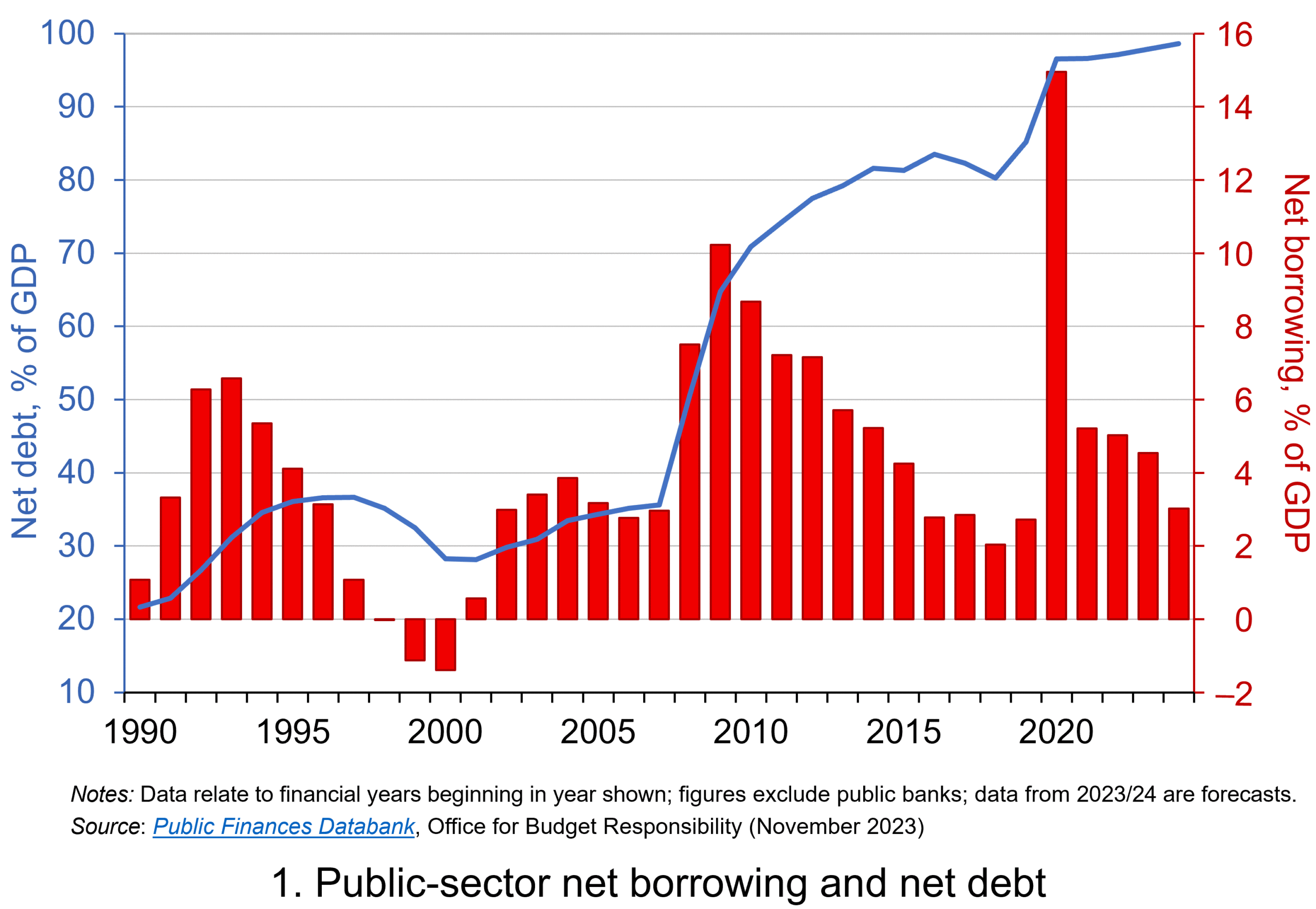 Chart 1 shows the path of UK public-sector net debt and net borrowing, as percentages of GDP, since 1990. Debt is a stock concept and is the result of accumulated flows of past borrowing. Net debt is simply gross debt less liquid financial assets, which mainly consist of foreign exchange reserves and cash deposits. Net borrowing is the headline measure of the sector’s deficit and is based on when expenditures and receipts (largely taxation) are recorded rather than when cash is actually paid or received. (Click here for a PowerPoint of Chart 1)
Chart 1 shows the impact of the fiscal interventions associated with the global financial crisis and the COVID-19 pandemic, when net borrowing rose to 10 per cent and 15 per cent of GDP respectively. The former contributed to the debt-to-GDP ratio rising from 35.6 per cent in 2007/8 to 81.6 per cent in 2014/15, while the pandemic and subsequent cost-of-living interventions contributed to the ratio rising from 85.2 per cent in 2019/20 to around 98 per cent in 2023/24.
Sustainability of the public finances
 The ratcheting up of debt levels affects debt servicing costs and hence the budgetary position of government. Yet the recent increases in interest rates also raise the costs faced by governments in financing future deficits or refinancing existing debts that are due to mature. In addition, a continuation of the low economic growth that has beset the UK economy since the global financial crisis also has implications for the burden imposed on the public sector by its debts, and hence the sustainability of the public finances. After all, low growth has implications for spending commitments, and, of course, the flow of receipts.
The analysis therefore implies that the sustainability of public-sector debt is dependent on at least three factors: existing debt levels, the implied average interest rate facing the public sector on its debts, and the rate of economic growth. These three factors turn out to underpin a well-known rule relating to the fiscal arithmetic of public-sector debt. The rule is sometimes known as the ‘r – g’ rule (i.e. the interest rate minus the growth rate).
Underpinning the fiscal arithmetic that determines the path of public-sector debt is the concept of the ‘primary balance’. This is the difference between the sector’s receipts and its expenditures less its debt interest payments. A primary surplus (a positive primary balance) means that receipts exceed expenditures less debt interest payments, whereas a primary deficit (a negative primary balance) means that receipts fall short. The fiscal arithmetic necessary to prevent the debt-to-GDP ratio rising produces the following stable debt equation or ‘r – g’ rule:
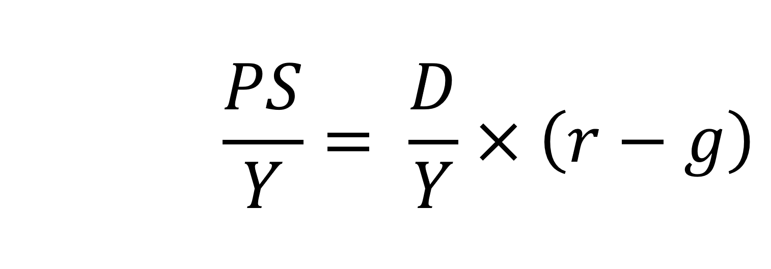
On the left-hand side of the stable debt equation is the required primary surplus (PS) to GDP (Y) ratio. Moving to the right-hand side, the first term is the existing debt-to-GDP ratio (D/Y). The second term ‘r – g’, is the differential between the average implied interest rate the government pays on its debt and the growth rate of the economy. These terms can be expressed in either nominal or real terms as this does not affect the differential.
To illustrate the rule consider a country whose existing debt-to-GDP ratio is 1 (i.e. 100 per cent) and the ‘r – g’ differential is 0.02 (2 percentage points). In this scenario they would need to run a primary surplus to GDP ratio of 0.02 (i.e. 2 percent of GDP).
The ‘r – g‘ differential
The ‘r – g’ differential reflects macroeconomic and financial conditions. The fiscal arithmetic shows that these are important for the dynamics of public-sector debt. The fiscal arithmetic is straightforward when r = g as any primary deficit will cause the debt-to-GDP ratio to rise, while a primary surplus will cause the ratio to fall. The larger is g relative to r the more favourable are the conditions for the path of debt. Importantly, if the differential is negative (r < g), it is possible for the public sector to run a primary deficit, up to the amount that the stable debt equation permits.
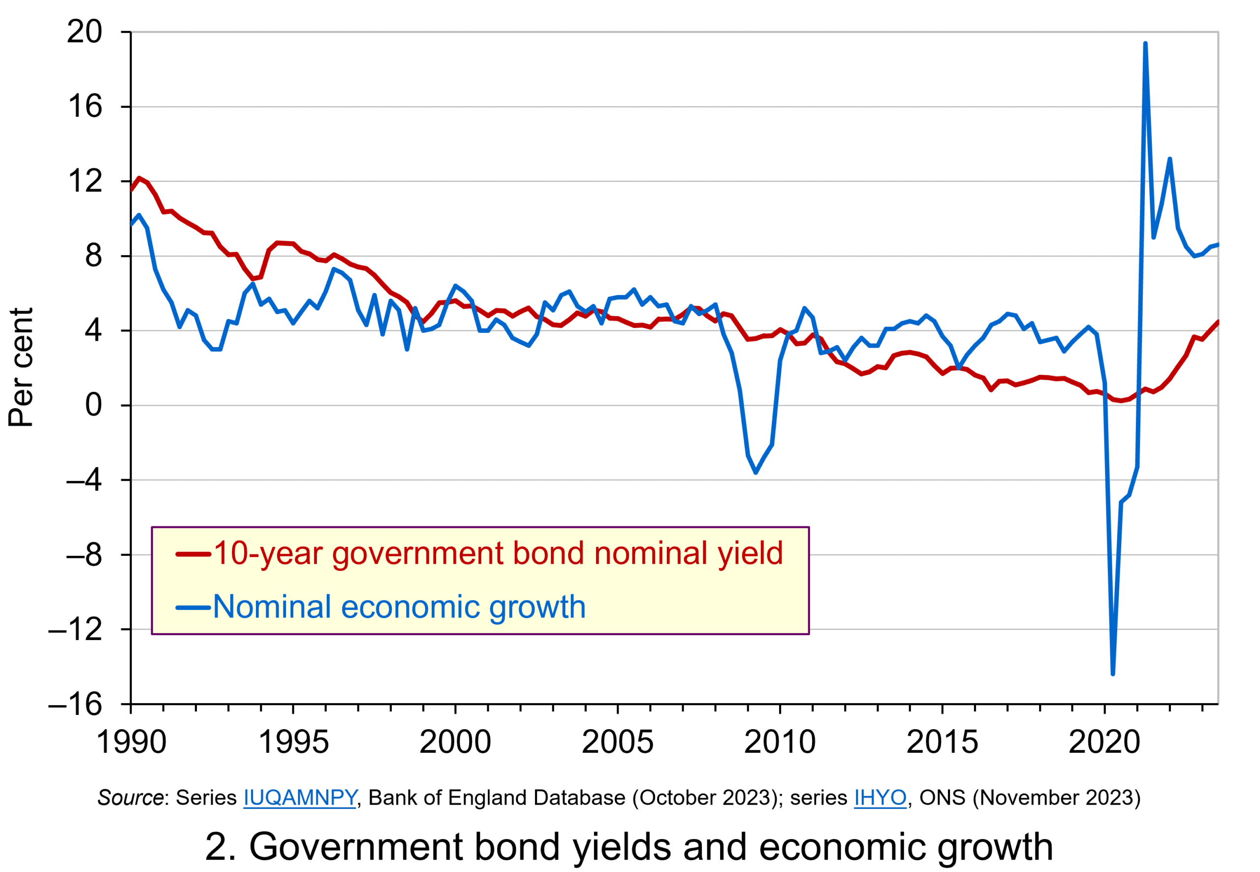 Consider Charts 2 and 3 to understand how the ‘r – g’ differential has affected debt sustainability in the UK since 1990. Chart 2 plots the implied yield on 10-year government bonds, alongside the annual rate of nominal growth (click here for a PowerPoint). As John explains in his blog The bond roller coaster, the yield is calculated as the coupon rate that would have to be paid for the market price of a bond to equal its face value. Over the period, the average annual nominal growth rate was 4.5 per cent, while the implied interest rate was almost identical at 4.6 per cent. The average annual rate of CPI inflation over this period was 2.8 per cent.
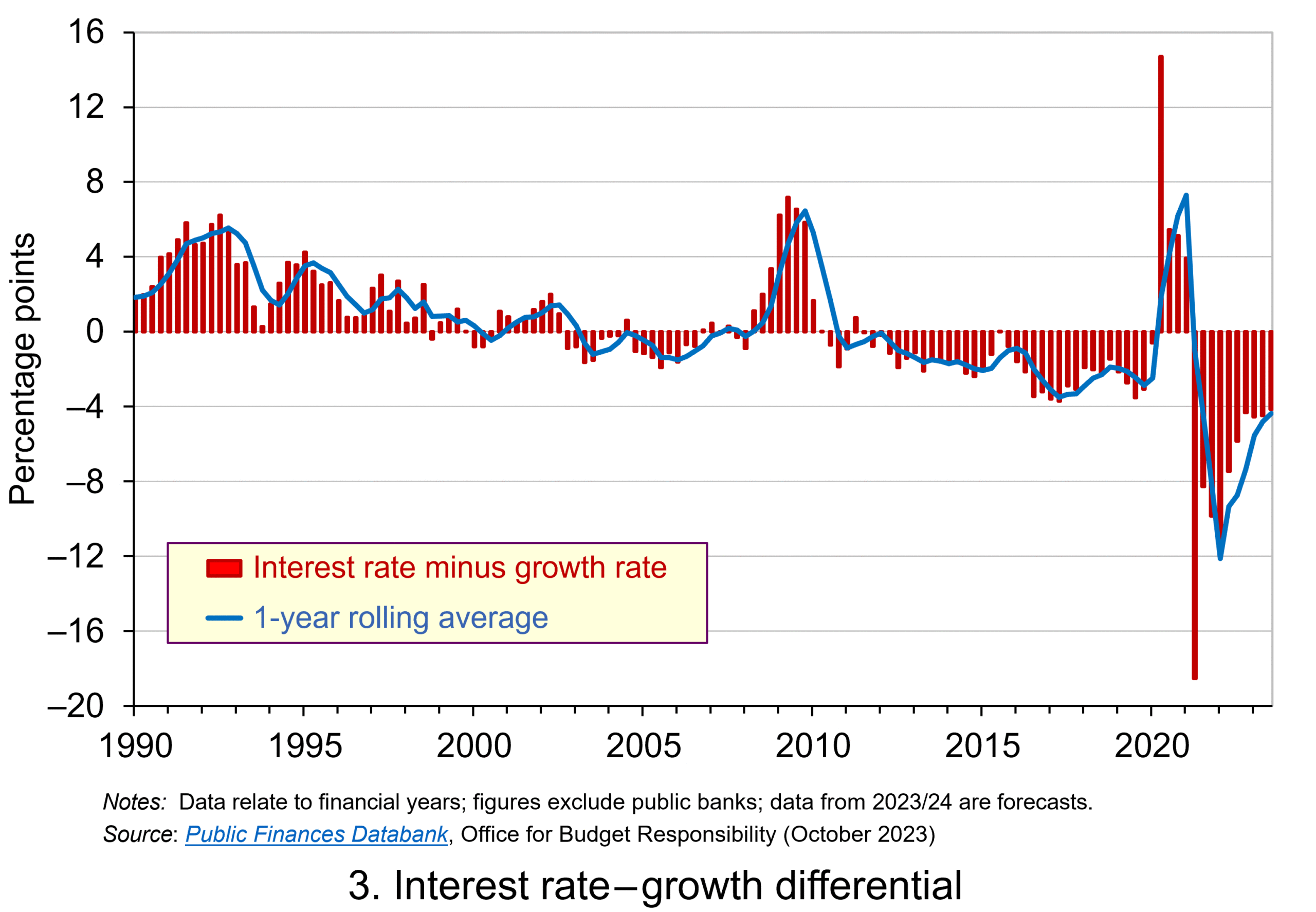 Chart 3 plots the ‘r – g’ differential which is simply the difference between the two series in Chart 2, along with a 12-month rolling average of the differential to help show better the direction of the differential by smoothing out some of the short-term volatility (click here for a PowerPoint). The differential across the period is a mere 0.1 percentage points implying that macroeconomic and financial conditions have typically been neutral in supporting debt sustainability. However, this does mask some significant changes across the period.
We observe a general downward trend in the ‘r – g’ differential from 1990 up to the time of the global financial crisis. Indeed between 2003 and 2007 we observe a favourable negative differential which helps to support the sustainability of public debt and therefore the well-being of the public finances. This downward trend of the ‘r – g’ differential was interrupted by the financial crisis, driven by a significant contraction in economic activity. This led to a positive spike in the differential of over 7 percentage points.
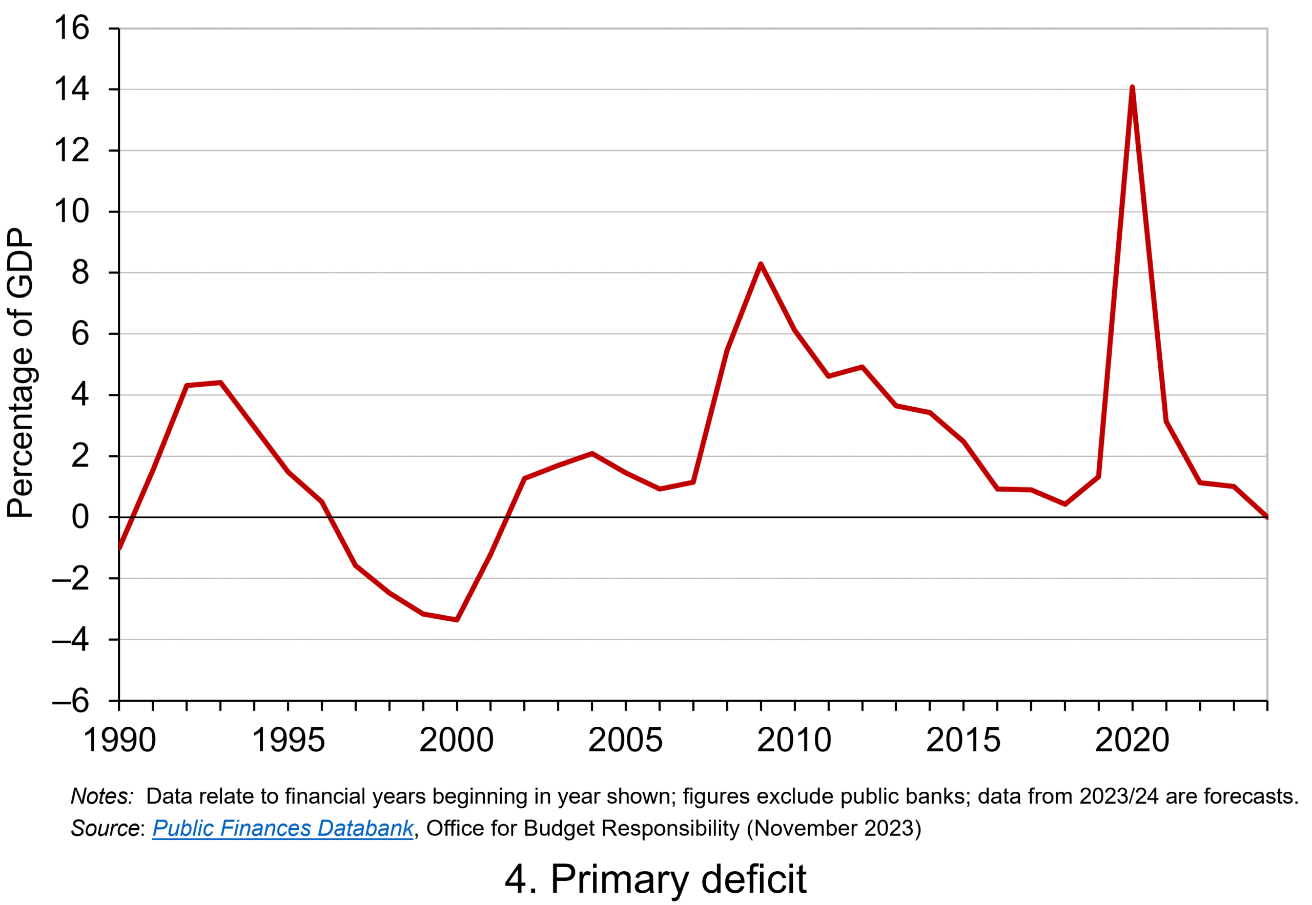 Yet the negative differential resumed in 2010 and continued up to the pandemic. Again, this is indicative of the macroeconomic and financial environments being supportive of the public finances. It was, however, largely driven by low interest rates rather than by economic growth.
Consequently, the negative ‘r – g’ differential meant that the public sector could continue to run primary deficits during the 2010s, despite the now much higher debt-to-GDP ratio. Yet, weak growth was placing limits on this. Chart 4 indeed shows that primary deficits fell across the decade (click here for a PowerPoint).
The pandemic and beyond
 The pandemic saw the ‘r – g’ differential again turn markedly positive, averaging 7 percentage points in the four quarters from Q2 of 2020. While the differential again turned negative, the debt-to-GDP ratio had also increased substantially because of large-scale fiscal interventions. This made the negative differential even more important for the sustainability of the public finances. The question is how long the negative differential can last.
Looking forward, the fiscal arithmetic is indeed uncertain and worryingly is likely to be less favourable. Interest rates have risen and, although inflationary pressures may be easing somewhat, interest rates are likely to remain much higher than during the past decade. Geopolitical tensions and global fragmentation pose future inflationary concerns and a further drag on growth.
As well as the short-term concerns over growth, there remain long-standing issues of low productivity which must be tackled if the growth of the UK economy’s potential output is to be raised. These concerns all point to the important ‘r – g’ differential become increasingly less negative, if not positive. If so the fiscal arithmetic could mean increasingly hard maths for policymakers.
Articles
- The budget deficit: a short guide
House of Commons Library (8/6/23)
- If markets are right about long real rates, public debt ratios will increase for some time. We must make sure that they do not explode.
Peterson Institute for International Economics, Olivier Blanchard (6/11/23)
- The UK government’s debt nightmare
ITV News, Robert Peston (13/7/23)
- National debt could hit 300% of GDP by 2070s, independent watchdog the OBR warns
Sky News, James Sillars (13/7/23)
- How much money is the UK government borrowing, and does it matter?
BBC News (20/10/23)
- Cost of national debt hits 20-year high
BBC News, Vishala Sri-Pathma & Faisal Islam (4/10/23)
- Bond markets could see ‘mini boom-bust cycles’ as global government debt to soar by $5 trillion a yea
Markets Insider, Filip De Mott (16/11/23)
- The counterintuitive truth about deficits for bond investors
Financial Times, Matt King (17/11/23)
- UK government borrowing almost £20bn lower than expected
The Guardian, Richard Partington (20/10/23)
- Controlling debt is just a means — it is not a government’s end
Financial Times, Martin Wolf (13/11/23)
Data
Questions
- What is meant by each of the following terms: (a) net borrowing; (b) primary deficit; (c) net debt?
- Explain how the following affect the path of the public-sector debt-to-GDP ratio: (a) interest rates; (b) economic growth; (c) the existing debt-to-GDP ratio.
- Which factors during the 2010s were affecting the fiscal arithmetic of public debt positively, and which negatively?
- Discuss the prospects for the fiscal arithmetic of public debt in the coming years.
- Assume that a country has an existing public-sector debt-to-GDP ratio of 60 percent.
(a) Using the ‘rule of thumb’ for public debt dynamics, calculate the approximate primary balance it would need to run in the coming year if the expected average real interest rate on the debt were 3 per cent and real economic growth were 2 per cent?
(b) Repeat (a) but now assume that real economic growth is expected to be 4 per cent.
(c) Repeat (a) but now assume that the existing public-sector debt-to-GDP ratio is 120 per cent.
(d) Using your results from (a) to (c) discuss the factors that affect the fiscal arithmetic of the growth of public-sector debt.
 In his blog, The bond roller coaster, John looks at the pricing of government bonds and details how, in recent times, governments wishing to borrow by issuing new bonds are having to offer higher coupon rates to attract investors. The interest rate hikes by central banks in response to global-wide inflationary pressures have therefore spilt over into bond markets. Though this evidences the ‘pass through’ of central bank interest rate increases to the general structure of interest rates, it does, however, pose significant costs for governments as they seek to finance future budgetary deficits or refinance existing debts coming up to maturity.
The Autumn Statement in the UK is scheduled to be made on 22 November. This, as well as providing an update on the economy and the public finances, is likely to include a number of fiscal proposals. It is thus timely to remind ourselves of the size of recent discretionary fiscal measures and their potential impact on the sustainability of the public finances. In this first of two blogs, we consider the former: the magnitude of recent discretionary fiscal policy changes.
First, it is important to define what we mean by discretionary fiscal policy. It refers to deliberate changes in government spending or taxation. This needs to be distinguished from the concept of automatic stabilisers, which relate to those parts of government budgets that automatically result in an increase (decrease) of spending or a decrease (increase) in tax payments when the economy slows (quickens).
The suitability of discretionary fiscal policy measures depends on the objectives they trying to fulfil. Discretionary measures can be implemented, for example, to affect levels of public-service provision, the distribution of income, levels of aggregate demand or to affect longer-term growth of aggregate supply. As we shall see in this blog, some of the large recent interventions have been conducted primarily to support and stabilise economic activity in the face of heightened economic volatility.
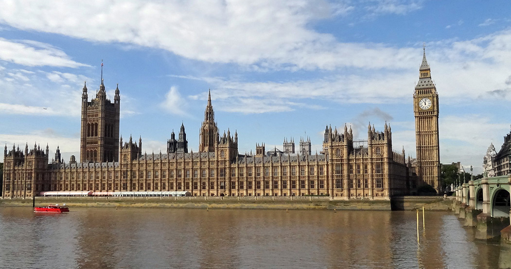 Discretionary fiscal measures in the UK are usually announced in annual Budget statements in the House of Commons. These are normally in March, but discretionary fiscal changes can be made in the Autumn Statement too. The Autumn Statement of October 2022, for example, took on significant importance as the new Chancellor of the Exchequer, Jeremy Hunt, tried to present a ‘safe pair hands’ following the fallout and market turbulence in response to the fiscal statement by the former Chancellor, Kwasi Kwarteng, on 23 September that year.
The fiscal impulse
The large-scale economic turbulence of recent years associated first with the global financial crisis of 2007–9 and then with the COVID-19 pandemic and the cost-of-living crisis, has seen governments respond with significant discretionary fiscal measures. During the COVID-19 pandemic, examples of fiscal interventions in the UK included the COVID-19 Business Interruption Loan Scheme (CBILS), grants for retail, hospitality and leisure businesses, the COVID-19 Job Retention Scheme (better known as the furlough scheme) and the Self-Employed Income Support Scheme.
 The size of discretionary fiscal interventions can be measured by the fiscal impulse. This captures the magnitude of change in discretionary fiscal policy and thus the size of the stimulus. The concept is not to be confused with fiscal multipliers, which measure the impact of fiscal changes on economic outcomes, such as real national income and employment.
By measuring fiscal impulses, we can analyse the extent to which a country’s fiscal stance has tightened, loosened, or remained unchanged. In other words, we are attempting to capture discretionary fiscal policy changes that result in structural changes in the government budget and, therefore, in structural changes in spending and/or taxation.
To measure structural changes in the public-sector’s budgetary position, we calculate changes in structural budget balances.
A budget balance is simply the difference between receipts (largely taxation) and spending. A budget surplus occurs when receipts are greater than spending, while a deficit (sometimes referred to as net borrowing) occurs if spending is greater than receipts.
A structural budget balance cyclically-adjusts receipts and spending and hence adjusts for the position of the economy in the business cycle. In doing so, it has the effect of adjusting both receipts and spending for the effect of automatic stabilisers. Another way of thinking about this is to ask what the balance between receipts and spending would be if the economy were operating at its potential output. A deterioration in a structural budget balance infers a rise in the structural deficit or fall in the structural surplus. This indicates a loosening of the fiscal stance. An improvement in the structural budget balance, by contrast, indicates a tightening.
The size of UK fiscal impulses
A frequently-used measure of the fiscal impulse involves the change in the cyclically-adjusted public-sector primary deficit.
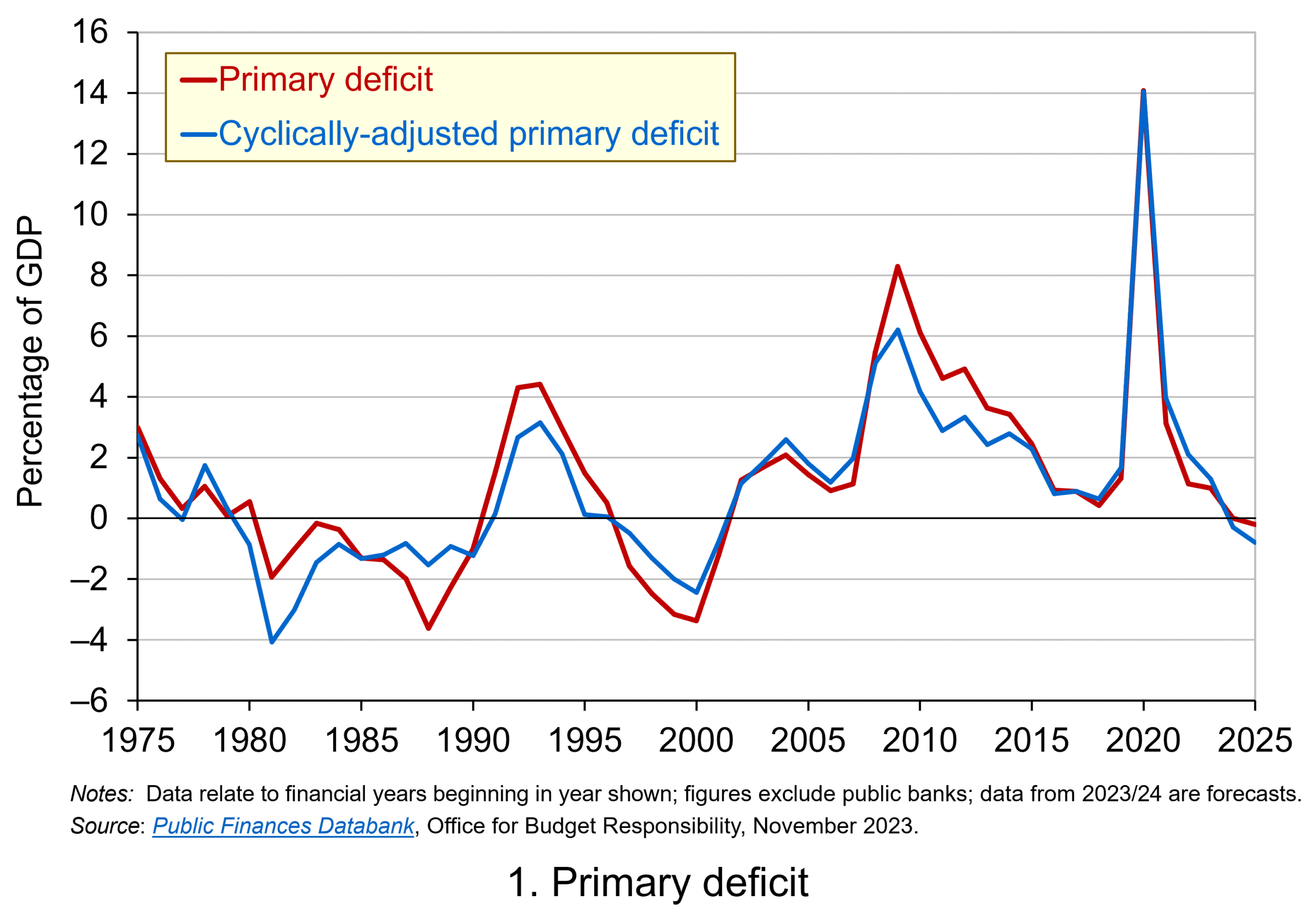 A primary deficit captures the extent to which the receipts of the public sector fall short of its spending, excluding its spending on debt interest payments. It essentially captures whether the public sector is able to afford its ‘new’ fiscal choices from its receipts; it excludes debt-servicing costs, which can be thought of as reflecting fiscal choices of the past. By using a cyclically-adjusted primary deficit we are able to isolate more accurately the size of discretionary policy changes. Chart 1 shows the UK’s actual and cyclically-adjusted primary deficit as a share of GDP since 1975, which have averaged 1.3 and 1.1 per cent of GDP respectively. (Click here for a PowerPoint of the chart.)
The size of the fiscal impulse is measured by the year-on-year percentage point change in the cyclically-adjusted public-sector primary deficit as a percentage of potential GDP. A larger deficit or a smaller surplus indicates a fiscal loosening (a positive fiscal impulse), while a smaller deficit or a larger surplus indicates a fiscal tightening (a negative fiscal impulse).
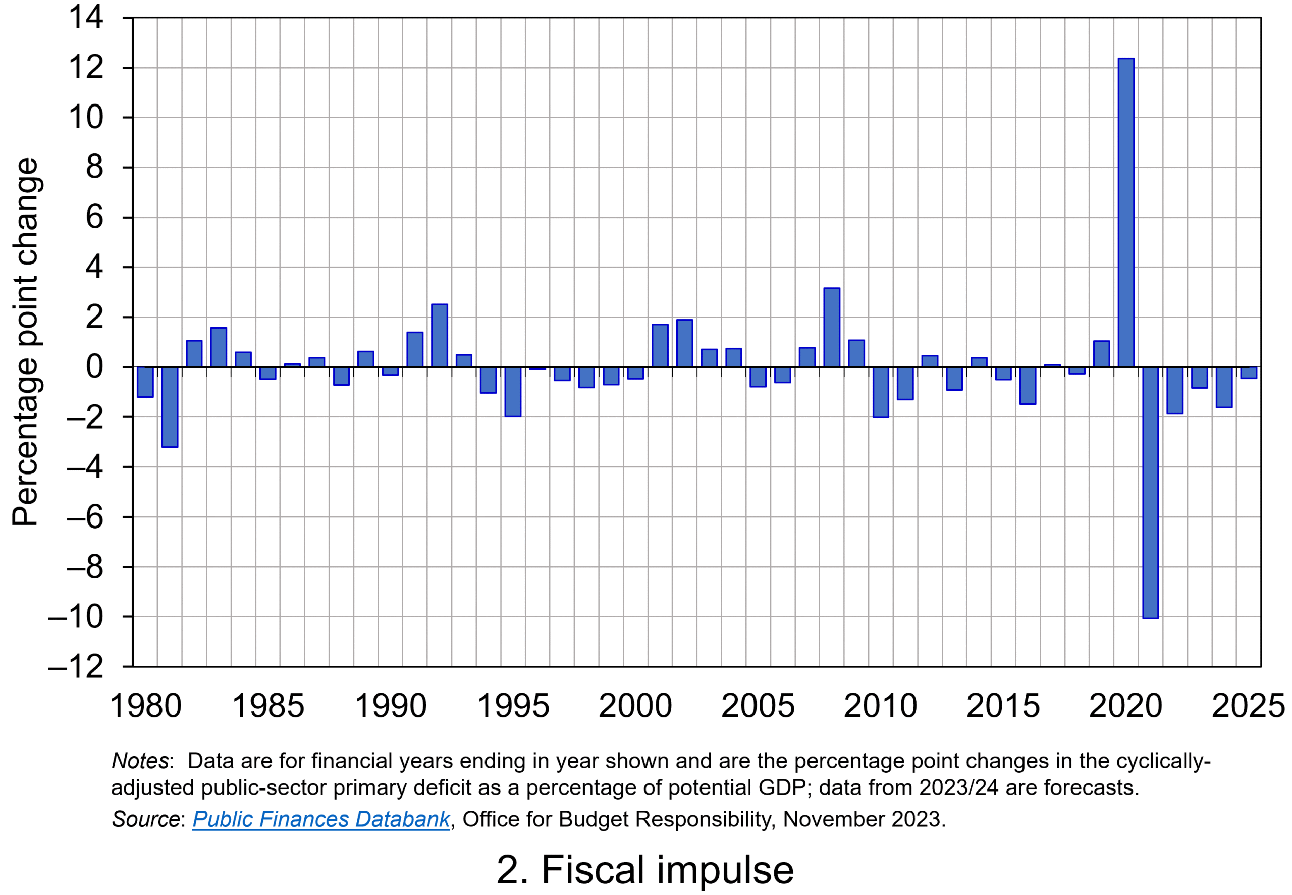 Chart 2 shows the magnitude of UK fiscal impulses since 1980. It captures very starkly the extent of the loosening of the fiscal stance in 2020 in response to the COVID-19 pandemic. (Click here for a PowerPoint of the chart.) In 2020 the cyclically-adjusted primary deficit to potential output ratio rose from 1.67 to 14.04 per cent. This represents a positive fiscal impulse of 12.4 per cent of GDP.
A tightening of fiscal policy followed the waning of the pandemic. 2021 saw a negative fiscal impulse of 10.1 per cent of GDP. Subsequent tightening was tempered by policy measures to limit the impact on the private sector of the cost-of-living crisis, including the Energy Price Guarantee and Energy Bills Support Scheme.
In comparison, the fiscal response to the global financial crisis led to a cumulative increase in the cyclically-adjusted primary deficit to potential GDP ratio from 2007 to 2009 of 5.0 percentage points. Hence, the financial crisis saw a positive fiscal impulse of 5 per cent of GDP. While smaller in comparison to the discretionary fiscal responses to the COVID-19 pandemic, it was, nonetheless, a sizeable loosening of the fiscal stance.
Sustainability and well-being of the public finances
The recent fiscal interventions have implications for the financial well-being of the public-sector. Not least, the financing of the positive fiscal impulses has led to a substantial growth in the accumulated size of the public-sector debt stock. At the end of 2006/7 the public-sector net debt stock was 35 per cent of GDP; at the end of the current financial year, 2023/24, it is expected to be 103 per cent.
As we saw at the outset, in an environment of rising interest rates, the increase in the public-sector debt to GDP ratio creates significant additional costs for government, a situation that is made more difficult for government not only by the current flatlining of economic activity, but by the low underlying rate of economic growth seen since the financial crisis. The combination of higher interest rates and lower economic growth has adverse implications for the sustainability of the public finances and the ability of the public sector to absorb the effects of future economic crises.
Articles
- Autumn Statement 2023: When is it and how will it affect me?
BBC News (16/11/23)
- What is the Autumn Statement?
House of Commons Library (13/11/23)
- Putting the fiscal toothpaste back into the tube: It’s time to normalise the euro area fiscal stance in 2024
VoxEU, Niels Thygesen, Roel Beetsma, Massimo Bordignon, Xavier Debrun, Mateusz Szczurek, Martin Larch, Matthias Busse, Mateja Gabrijelcic, Laszlo Jankovics and Janis Malzubris (30/6/23)
- Euro zone should tighten fiscal policy in 2024 to curb inflation, European Fiscal Board says
Reuters, Jan Strupczewski (28/6/23)
- Hutchins Center Fiscal Impact Measure: Federal, State and Local Fiscal Policy and the Economy
Brookings, Eli Asdourian, Louise Sheiner, and Lorae Stojanovic (27/10/23)
Report
- IFS Green Budget
Institute for Fiscal Studies, Carl Emmerson, Paul Johnson and Ben Zaranko (eds) (October 2023)
Data
Questions
- Explain what is meant by the following fiscal terms: (a) structural deficit; (b) automatic stabilisers; (c) discretionary fiscal policy; (d) primary deficit.
- What is the difference between current and capital public expenditures? Give some examples of each.
- Consider the following two examples of public expenditure: grants from government paid to the private sector for the installation of energy-efficient boilers, and welfare payments to unemployed people. How are these expenditures classified in the public finances and what fiscal objectives do you think they meet?
- Which of the following statements about the primary balance is FALSE?
(a) In the presence of debt interest payments a primary deficit will be smaller than a budget deficit.
(b) In the presence of debt interest payments a primary surplus will be smaller than a budget surplus.
(c) The primary balance differs from the budget balance by the size of debt interest payments.
(d) None of the above.
- Explain the difference between a fiscal impulse and a fiscal multiplier.
- Why is low economic growth likely to affect the sustainability of the public finances? What other factors could also matter?
 We have examined inflation in several blogs in recent months. With inflation at levels not seen for 40 years, this is hardly surprising. One question we’ve examined is whether the policy response has been correct. For example, in July, we asked whether the Bank of England had raised interest rates too much, too late. In judging policy, one useful distinction is between demand-pull inflation and cost-push inflation. Do they require the same policy response? Is raising interest rates to get inflation down to the target rate equally applicable to inflation caused by excessive demand and inflation caused by rising costs, where those rising costs are not caused by rising demand?
In terms of aggregate demand and supply, demand-pull inflation is shown by continuing rightward shifts in aggregate demand (AD); cost-push inflation is shown by continuing leftward/upward shifts in short-run aggregate supply (SRAS). This is illustrated in the following diagram, which shows a single shift in aggregate demand or short-run aggregate supply. For inflation to continue, rather than being a single rise in prices, the curves must continue to shift.
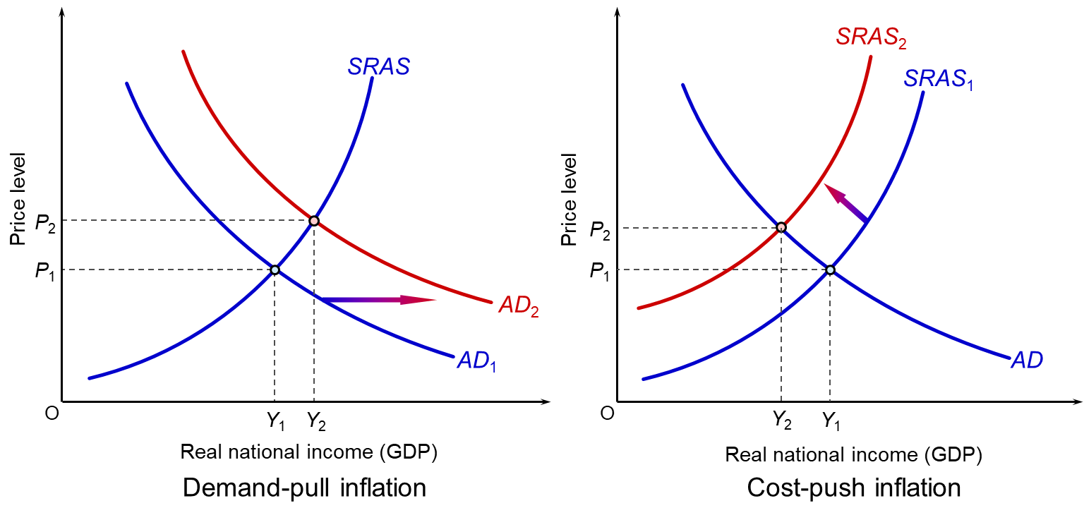
As you can see, the effects on real GDP (Y) are quite different. A rise in aggregate demand will tend to increase GDP (as long as capacity constraints allow). A rise in costs, and hence an upward shift in short-run aggregate supply, will lead to a fall in GDP as firms cut output in the face of rising costs and as consumers consume less as the cost of living rises.
The inflation experienced by the UK and other countries in recent months has been largely of the cost-push variety. Causes include: supply-chain bottlenecks as economies opened up after COVID-19; the war in Ukraine and its effects on oil and gas supplies and various grains; and avian flu and poor harvests from droughts and floods associated with global warming resulting in a fall in food supplies. These all led to a rise in prices. In the UK’s case, this was compounded by Brexit, which added to firms’ administrative costs and, according to the Bank of England, was estimated to cause a long-term fall in productivity of around 3 to 4 per cent.
The rise in costs had the effect of shifting short-run aggregate supply upwards to the left. As well as leading to a rise in prices and a cost-of-living squeeze, the rising costs dampened expenditure.
This was compounded by a tightening of fiscal policy as governments attempted to tackle public-sector deficits and debt, which had soared with the support measures during the pandemic. It was also compounded by rising interest rates as central banks attempted to bring inflation back to target.
Monetary policy response
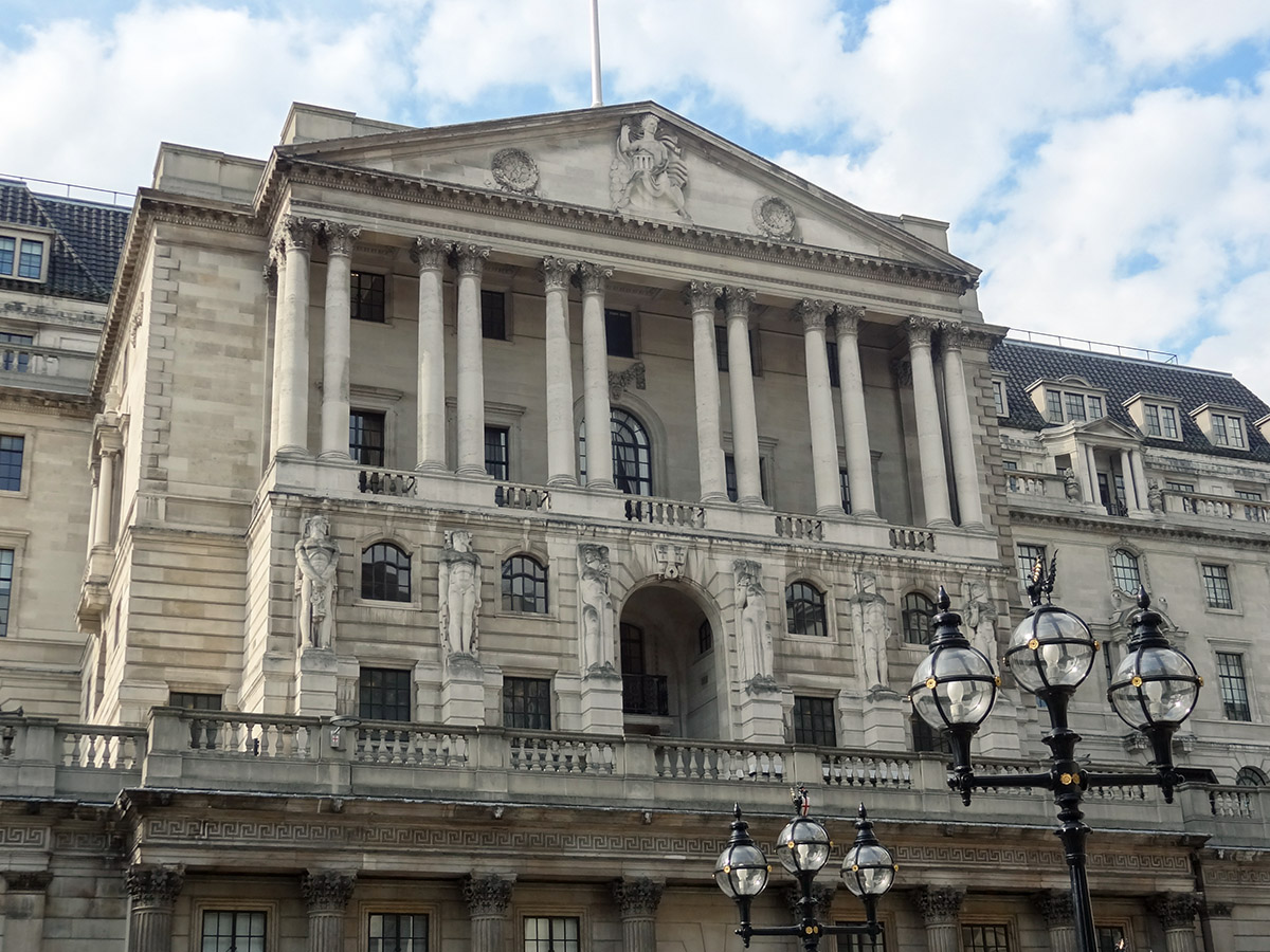 Central banks are generally charged with keeping inflation in the medium term at a target rate set by the government or the central bank itself. For most developed countries, this is 2% (see table in the blog, Should central bank targets be changed?). So is raising interest rates the correct policy response to cost-push inflation?
One argument is that monetary policy is inappropriate in the face of supply shocks. The supply shocks themselves have the effect of dampening demand. Raising interest rates will compound this effect, resulting in lower growth or even a recession. If the supply shocks are temporary, such as supply-chain disruptions caused by lockdowns during the pandemic, then it might be better to ride out the problem and not raise interest rates or raise them by only a small amount. Already cost pressures are easing in some areas as supplies have risen.
If, however, the fall in aggregate supply is more persistent, such as from climate-related declines in harvests or the Ukraine war dragging on, or new disruptions to supply associated with the Israel–Gaza war, or, in the UK’s case, with Brexit, then real aggregate demand may need to be reduced in order to match the lower aggregate supply. Or, at the very least, the growth in aggregate demand may need to be slowed to match the slower growth in aggregate supply.
Huw Pill, the Chief Economist at the Bank of England, in a podcast from the Columbia Law School (see links below), argued that people should recognise that the rise in costs has made them poorer. If they respond to the rising costs by seeking higher wages, or in the case of businesses, by putting up prices, this will simply stoke inflation. In these circumstances, raising interest rates to cool aggregate demand may reduce people’s ability to gain higher wages or put up prices.
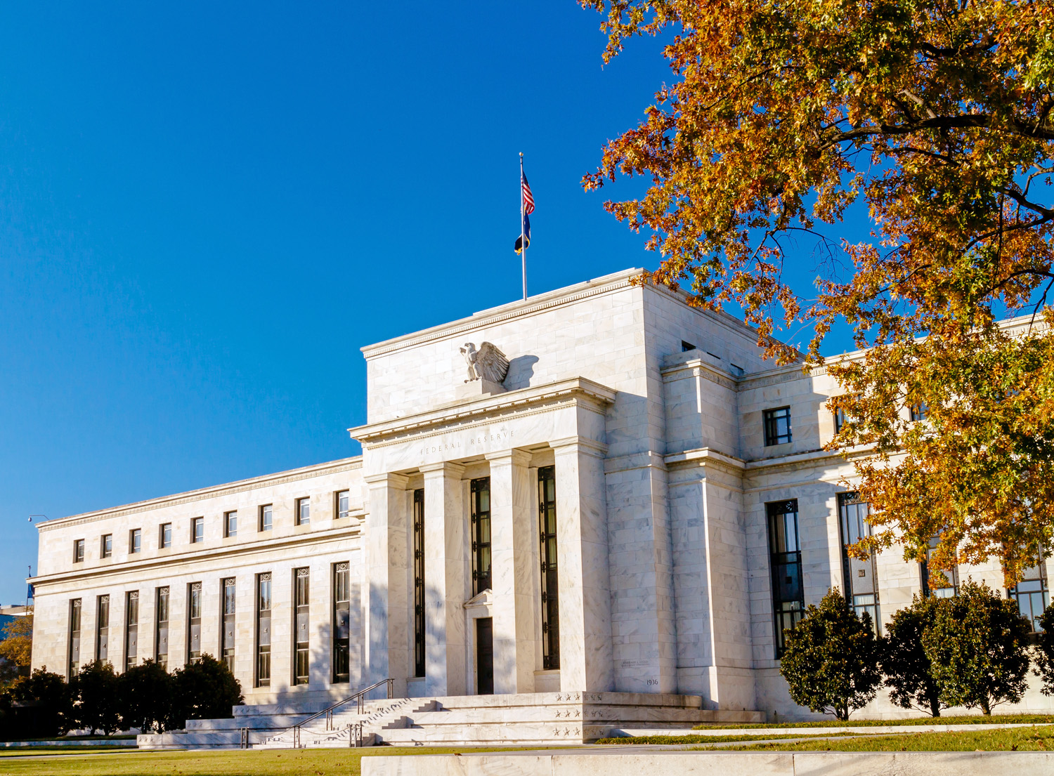 Another argument for raising interest rates in the face of cost-push inflation is when those cost increases are felt more than in other countries. The USA has suffered less from cost pressures than the UK. On the other hand, its growth rate is higher, suggesting that its inflation, albeit lower than in the UK, is more of the demand-pull variety. Despite its inflation rate being lower than in the UK, the problem of excess demand has led the Fed to adopt an aggressive interest rate policy. Its target rate is 5.25% to 5.50%, while the Bank of England’s is 5.25%. In order to prevent short-term capital outflows and a resulting depreciation in the pound, further stoking inflation, the Bank of England has been under pressure to mirror interest rate rises in the USA, the eurozone and elsewhere.
Articles
Blogs on this site
Information and data
Questions
- How may monetary policy affect inflationary expectations?
- If cost-push inflation makes people generally poorer, what role does the government have in making the distribution of a cut in real income a fair one?
- In the context of cost-push inflation, how might the authorities prevent a wage–price spiral?
- With reference to the second article above, explain the ‘monetary policy conundrum’ faced by the Bank of Japan.
- If central banks have a single policy instrument, namely changes in interest rates, how may conflicts arise when there is more than one macroeconomic objective?
- Is Russia’s rise in inflation the result of cost or demand pressures, or a mixture of the two (see articles above)?
 The distinction between nominal and real values in one of the ‘threshold concepts’ in economics. These are concepts that are fundamental to a discipline and which occur again and again. The distinction between nominal and real values is particularly important when interpreting and analysing data. We show its importance here when analysing the latest retail sales data from the Office for National Statistics.
Retail sales relate to spending on items such as food, clothing, footwear, and household goods (see). They involve sales by retailers directly to end consumers whether in store or online. The retail sales index for Great Britain is based on a monthly survey of around 5000 retailers across England, Scotland and Wales and is thought to capture around 93 per cent of turnover in the sector.
Estimates of retail sales are published in index form. There are two indices published by the ONS: a value and volume measure. The value index reflects the total turnover of business, while the volume index adjusts the value index for price changes. Hence, the value estimates are nominal, while the volume estimates are real. The key point here is that the nominal estimates reflect both price and volume changes, whereas the real estimates adjust for price movements to capture only volume changes.
The headline ONS figures for September 2023 showed a 0.9 per cent volume fall in the volume of retail sales, following a 0.4 per cent rise in August. In value terms, September saw a 0.2 per cent fall in retail sales following a 0.9 per cent rise in August. Monthly changes can be quite volatile, even after seasonal adjustment, and sensitive to peculiar factors. For example, the unusually warm weather this September helped to depress expenditure on clothes. It is, therefore, sensible to take a longer-term view when looking for clearer patterns in spending behaviour.
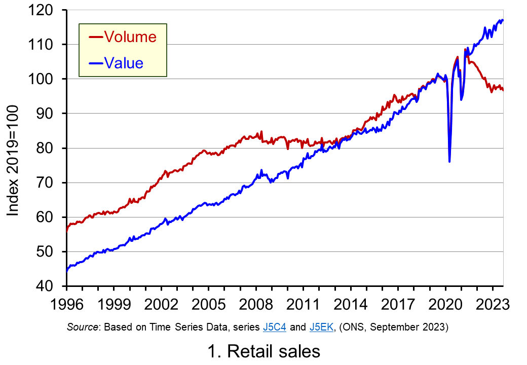 Chart 1 plots the value and volume of retail sales in Great Britain since 1996. (Click here for a PowerPoint of this and the other two charts). In value terms, retail sales spending increased by 165 per cent, whereas in volume terms, spending increased by 73 per cent. This difference is expected in the presence of rising prices, since nominal growth, as we have just noted, reflects both price and volume changes. The chart is notable for capturing two periods where the volume of retail spending ceased to grow. The first of these is following the global financial crisis of the late 2000s. The period from 2008 to 2013 saw the volume of retail sales stagnate and flatline with a recovery in volumes only really starting to take hold in 2014. Yet in nominal terms retail sales grew by around 16 per cent.
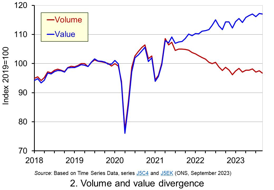 The second of the two periods is the decline in the volume of retail sales from 2021. To help illustrate this more clearly, Chart 2 zooms in on retail sales over the past five years or so. We can see a significant divergence between the volume and value of retail sales. Between April 2021 and September 2023, the volume of retail sales fell by 11%. In contrast, the value of retail sales increased by 8.4%. The impact of the inflationary shock and the consequent cost-of-living crisis that emerged from 2021 is therefore demonstrated starkly by the chart, not least the severe drag that it has had on the volume of retail spending. This has meant that the aggregate volume of retail sales in September 2023 was only back to the levels of mid-2018.
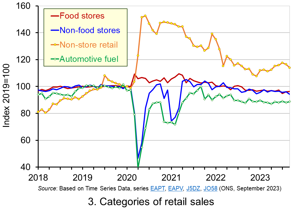 Finally, Chart 3 shows the patterns in the volumes of retailing by four categories since 2018: specifically, food stores, predominantly non-food stores, non-store retail, and automotive fuel. The largest fall in the volume of retail sales has been experienced by non-store retailing – largely online retailing. From its peak in December 2021, non-store retail sales decreased by 18% up to September 2023. While this needs to be set in the context of the volume of non-store retail purchases being 15% higher than in February 2020 before the pandemic lockdowns were introduced, it is nonetheless indicative of the pressures facing online retailers.
Importantly, the final chart shows that the pressures in retailing are widespread. Spending volumes on automotive fuels, and in food and non-food stores are all below 2019 levels. The likelihood is that these pressures will persist for some time to come. This inevitably has potential implications for retailers and, of course, for those that work in the sector.
Articles
Statistical bulletin
Data
Questions
- Why does an increase in the value of retail sales not necessarily mean that their volume has increased?
- In the presence of deflation, which will be higher: nominal or real growth rates?
- Discuss the factors that could explain the patterns in the volume of spending observed in the different categories of retail sales in Chart 3.
- Discuss what types of retail products might be more or less sensitive to the macroeconomic environment.
- Conduct a survey of recent media reports to prepare a briefing discussing examples of retailers who have struggled or thrived in the recent economic environment.
- What do you understand by the concepts of ‘consumer confidence’ and ‘economic uncertainty’? How might these affect the volume of retail spending?
- Discuss the proposition that the retail sales data cast doubt on whether people are ‘forward-looking consumption smoothers’.
 Have you ever wondered how your job affects your happiness? We all know that not all jobs are created equal. Some are awesome, while others … not so much. Well, it turns out that employment status and the type of work you do can have a big impact on how you feel – especially in developing countries where labour markets are usually tighter and switching between jobs can be more difficult.
A recent study by Carmichael, Darko and Vasilakos (2021) uses survey data from Ethiopia, Peru, India and Vietnam to answer this very question. The study found that the quality of work is a big deal when it comes to how young people feel. Not all jobs are ‘good jobs’ that automatically make you feel great. Although your wellbeing is likely to be higher when you’re in employment than when you’re not, there are certain job attributes that can push that ‘employment premium’ up or down. This is especially important to understand in countries like many in sub-Saharan Africa, where there aren’t many formal jobs, and people often end up overqualified for what they do.
What job attributes lead to higher wellbeing?
 What then are the job attributes that are correlated with higher levels of wellbeing? The first is money: Okay, we know money can’t buy happiness, but it can certainly make life easier. We were therefore hardly surprised to find a positive and statistically significant association between hourly earnings and wellbeing.
We were also not surprised to find that a ‘poor working environment’ has a strong and highly significant negative effect on wellbeing.
Finally, feeling proud of your work is also found to be a strongly significant determinant of your wellbeing. After all, people tend to excel in things they like doing, which is probably part of the ‘transmission mechanism’ between ‘work pride’ and ‘subjective wellbeing’.
 Which one of these attributes did you think had the greatest effect on wellbeing? Let me guess, many of you will say ‘earnings’. But then you would be wrong. Earnings were indeed positively associated with wellbeing and statistically significant at just about the 10% level, whereas work pride was very strongly statistically significant at the 1% level and had an effect on wellbeing that was four times greater than hourly earnings.
Putting yourself in a poor working environment on the other hand would reduce your wellbeing by almost twice as much as the earnings coefficient.
Policy implications
What does all this mean for policy-makers? If we want to make life better for young people in low-income countries, we need to tackle the problems from multiple angles.
 First, young people need to be helped to get the skills they need for the job market. This can be done through things like training programmes and apprenticeships. However, not all of these programmes are created equal. Some have great results, and others not so much.
But that’s not the whole story. In many countries, there’s a massive informal job market. It’s a place where people work but often don’t have the rights or protections that formal employees do. So, even if young people get trained, they might not find the ‘good’ jobs they’re hoping for.
Changes also need to be made on a much bigger scale. This often includes decentralising public investment to include rural areas, improving infrastructure, and encouraging private investment. Strengthening labour market rules and social protection can help too, by making sure that work is safe and fair.
In a nutshell, where you work and what kind of work you do can make a big difference to how you feel.
Conclusions
If policy-makers want to help young people in low-income countries, they need both to give them the skills they require and to create better job opportunities. But policy-makers also need to make bigger changes to the way things work, like boosting production and making sure jobs are safe and fair.
In the end, it’s about making life better for young people around the world. Let’s keep working on it!
Articles
- Well-being and employment of young people in Ethiopia, India, Peru and Vietnam: Is work enough?
Development Policy Review, Fiona Carmichael, Christian K. Darko and Nicholas Vasilakos (18/5/21)
- The search for ‘meaning’ at work
BBC Worklife, Kate Morgan (7/9/22)
- Job Satisfaction Is Rising: What’s Behind The Surprising Tend
Forbes, Tracy Brower (4/6/23)
- Young workers are embracing AI, job satisfaction rising: 2023 Young Generation in Tech report
Silicon Canals (4/10/23)
- ‘These jobs can be respectable too’: Why youths in China are abandoning white-collar jobs for ‘light labor’
CNBC, Goh Chiew Tong (6/6/23)
- Does Work Make You Happy? Evidence from the World Happiness Report
Harvard Business Review, Jan-Emmanuel De Neve and George Ward (20/3/17)
- Worker well-being is in demand as organizational culture shifts
American Psychological Association, Monitor on Psychology, Heather Stringer (1/1/23)
- Understanding children’s work and youth employment outcomes in Indonesia
Understanding Children’s Work (UCW) Programme, Villa Aldobrandini and V. Panisperna (June 2012)
- Where are We with Young People’s Wellbeing? Evidence from Nigerian Demographic and Health Surveys 2003–2013
Social Indicators Research, pp.803–33, Boniface Ayanbekongshie Ushie and Ekerette Emmanuel Udoh (November 2016)
- Employment Status and Well-Being Among Young Individuals. Why Do We Observe Cross-Country Differences?
Social Indicators Research, Dominik Buttler (29/6/22)
- Employment Mismatches Drive Expectational Earnings Errors among Mozambican Graduates
The World Bank Economic Review, Sam Jones, Ricardo Santos and Gimelgo Xirinda (27/7/23)
- Youth Employment and Skills Development in The Gambia
World Bank Working Paper 217, Nathalie Lahire, Richard Johanson and Ryoko Tomita Wilcox (2011)
Questions
- How does the quality of work impact the happiness and wellbeing of young people in low- and middle-income countries (LMICs), and why is this significant in the context of job opportunities in sub-Saharan Africa?
- What are some potential solutions and strategies discussed in the article for improving the wellbeing of young people in LMICs, particularly in the context of employment and job opportunities?
- Have you ever experienced a job that significantly (positively or negatively) impacted your wellbeing or happiness? Reflect on your experience and how it influenced your overall life satisfaction?
- How is AI likely to affect the wellbeing of young professional workers?
- How is the pandemic likely to have affected job satisfaction?
 The past decade or so has seen large-scale economic turbulence. As we saw in the blog Fiscal impulses, governments have responded with large fiscal interventions. The COVID-19 pandemic, for example, led to a positive fiscal impulse in the UK in 2020, as measured by the change in the structural primary balance, of over 12 per cent of national income.
  Chart 1 shows the path of UK public-sector net debt and net borrowing, as percentages of GDP, since 1990. Debt is a stock concept and is the result of accumulated flows of past borrowing. Net debt is simply gross debt less liquid financial assets, which mainly consist of foreign exchange reserves and cash deposits. Net borrowing is the headline measure of the sector’s deficit and is based on when expenditures and receipts (largely taxation) are recorded rather than when cash is actually paid or received. (Click here for a PowerPoint of Chart 1)
 The ratcheting up of debt levels affects debt servicing costs and hence the budgetary position of government. Yet the recent increases in interest rates also raise the costs faced by governments in financing future deficits or refinancing existing debts that are due to mature. In addition, a continuation of the low economic growth that has beset the UK economy since the global financial crisis also has implications for the burden imposed on the public sector by its debts, and hence the sustainability of the public finances. After all, low growth has implications for spending commitments, and, of course, the flow of receipts.
 Consider Charts 2 and 3 to understand how the ‘r – g’ differential has affected debt sustainability in the UK since 1990. Chart 2 plots the implied yield on 10-year government bonds, alongside the annual rate of nominal growth (click here for a PowerPoint). As John explains in his blog The bond roller coaster, the yield is calculated as the coupon rate that would have to be paid for the market price of a bond to equal its face value. Over the period, the average annual nominal growth rate was 4.5 per cent, while the implied interest rate was almost identical at 4.6 per cent. The average annual rate of CPI inflation over this period was 2.8 per cent.
 Chart 3 plots the ‘r – g’ differential which is simply the difference between the two series in Chart 2, along with a 12-month rolling average of the differential to help show better the direction of the differential by smoothing out some of the short-term volatility (click here for a PowerPoint). The differential across the period is a mere 0.1 percentage points implying that macroeconomic and financial conditions have typically been neutral in supporting debt sustainability. However, this does mask some significant changes across the period.
  Yet the negative differential resumed in 2010 and continued up to the pandemic. Again, this is indicative of the macroeconomic and financial environments being supportive of the public finances. It was, however, largely driven by low interest rates rather than by economic growth.
  The pandemic saw the ‘r – g’ differential again turn markedly positive, averaging 7 percentage points in the four quarters from Q2 of 2020. While the differential again turned negative, the debt-to-GDP ratio had also increased substantially because of large-scale fiscal interventions. This made the negative differential even more important for the sustainability of the public finances. The question is how long the negative differential can last.
 In his blog,
  Discretionary fiscal measures in the UK are usually announced in annual Budget statements in the House of Commons. These are normally in March, but discretionary fiscal changes can be made in the Autumn Statement too. The Autumn Statement of October 2022, for example, took on significant importance as the new Chancellor of the Exchequer, Jeremy Hunt, tried to present a ‘safe pair hands’ following the fallout and market turbulence in response to the fiscal statement by the former Chancellor, Kwasi Kwarteng, on 23 September that year.
 The size of discretionary fiscal interventions can be measured by the fiscal impulse. This captures the magnitude of change in discretionary fiscal policy and thus the size of the stimulus. The concept is not to be confused with fiscal multipliers, which measure the impact of fiscal changes on economic outcomes, such as real national income and employment.
  A primary deficit captures the extent to which the receipts of the public sector fall short of its spending, excluding its spending on debt interest payments. It essentially captures whether the public sector is able to afford its ‘new’ fiscal choices from its receipts; it excludes debt-servicing costs, which can be thought of as reflecting fiscal choices of the past. By using a cyclically-adjusted primary deficit we are able to isolate more accurately the size of discretionary policy changes. Chart 1 shows the UK’s actual and cyclically-adjusted primary deficit as a share of GDP since 1975, which have averaged 1.3 and 1.1 per cent of GDP respectively. (Click
  Chart 2 shows the magnitude of UK fiscal impulses since 1980. It captures very starkly the extent of the loosening of the fiscal stance in 2020 in response to the COVID-19 pandemic. (Click
  We have examined inflation in several blogs in recent months. With inflation at levels not seen for 40 years, this is hardly surprising. One question we’ve examined is whether the policy response has been correct. For example, in July, we asked whether the Bank of England had raised interest rates
 Central banks are generally charged with keeping inflation in the medium term at a target rate set by the government or the central bank itself. For most developed countries, this is 2% (see table in the blog,
  Another argument for raising interest rates in the face of cost-push inflation is when those cost increases are felt more than in other countries. The USA has suffered less from cost pressures than the UK. On the other hand, its growth rate is higher, suggesting that its inflation, albeit lower than in the UK, is more of the demand-pull variety. Despite its inflation rate being lower than in the UK, the problem of excess demand has led the Fed to adopt an aggressive interest rate policy. Its target rate is 5.25% to 5.50%, while the Bank of England’s is 5.25%. In order to prevent short-term capital outflows and a resulting depreciation in the pound, further stoking inflation, the Bank of England has been under pressure to mirror interest rate rises in the USA, the eurozone and elsewhere.
 The distinction between nominal and real values in one of the ‘threshold concepts’ in economics. These are concepts that are fundamental to a discipline and which occur again and again. The distinction between nominal and real values is particularly important when interpreting and analysing data. We show its importance here when analysing the latest retail sales data from the Office for National Statistics.
 Chart 1 plots the value and volume of retail sales in Great Britain since 1996. (Click
  The second of the two periods is the decline in the volume of retail sales from 2021. To help illustrate this more clearly, Chart 2 zooms in on retail sales over the past five years or so. We can see a significant divergence between the volume and value of retail sales. Between April 2021 and September 2023, the volume of retail sales fell by 11%. In contrast, the value of retail sales increased by 8.4%. The impact of the inflationary shock and the consequent cost-of-living crisis that emerged from 2021 is therefore demonstrated starkly by the chart, not least the severe drag that it has had on the volume of retail spending. This has meant that the aggregate volume of retail sales in September 2023 was only back to the levels of mid-2018.
 Finally, Chart 3 shows the patterns in the volumes of retailing by four categories since 2018: specifically, food stores, predominantly non-food stores, non-store retail, and automotive fuel. The largest fall in the volume of retail sales has been experienced by non-store retailing – largely online retailing. From its peak in December 2021, non-store retail sales decreased by 18% up to September 2023. While this needs to be set in the context of the volume of non-store retail purchases being 15% higher than in February 2020 before the pandemic lockdowns were introduced, it is nonetheless indicative of the pressures facing online retailers.
  Have you ever wondered how your job affects your happiness? We all know that not all jobs are created equal. Some are awesome, while others … not so much. Well, it turns out that employment status and the type of work you do can have a big impact on how you feel – especially in developing countries where labour markets are usually tighter and switching between jobs can be more difficult.
 What then are the job attributes that are correlated with higher levels of wellbeing? The first is money: Okay, we know money can’t buy happiness, but it can certainly make life easier. We were therefore hardly surprised to find a positive and statistically significant association between hourly earnings and wellbeing.
 Which one of these attributes did you think had the greatest effect on wellbeing? Let me guess, many of you will say ‘earnings’. But then you would be wrong. Earnings were indeed positively associated with wellbeing and statistically significant at just about the 10% level, whereas work pride was very strongly statistically significant at the 1% level and had an effect on wellbeing that was four times greater than hourly earnings.
 First, young people need to be helped to get the skills they need for the job market. This can be done through things like training programmes and apprenticeships. However, not all of these programmes are created equal. Some have great results, and others not so much.